Using Visible Spectral Information to Predict Long-Wave Infrared Spectral Emissivity: A Case Study over the Sokolov Area of the Czech Republic with an Airborne Hyperspectral Scanner Sensor

Abstract

Remote-sensing platforms are often comprised of a cluster of different spectral range detectors or sensors to benefit from the spectral identification capabilities of each range. Missing data from these platforms, caused by problematic weather conditions, such as clouds, sensor failure, low temporal coverage or a narrow field of view (FOV), is one of the problems preventing proper monitoring of the Earth. One of the possible solutions is predicting a detector or sensor’s missing data using another detector/sensor. In this paper, we propose a new method of predicting spectral emissivity in the long-wave infrared (LWIR) spectral region using the visible (VIS) spectral region. The proposed method is suitable for two main scenarios of missing data: sensor malfunctions and narrow FOV. We demonstrate the usefulness and limitations of this prediction scheme using the airborne hyperspectral scanner (AHS) sensor, which consists of both VIS and LWIR spectral regions, in a case study over the Sokolov area, Czech Republic.

1. Introduction

Missing data in remote-sensing images result in only a partial understanding and interpretation of physical and biophysical processes or anthropogenic-based changes. There are several types and causes of missing data, such as problematic atmospheric conditions, like clouds [1–4], low temporal coverage [5] and temporary or permanent malfunctioning of the sensor or its communication system [6], saturated or malfunctioning bands [7] and saturated or malfunctioning pixels [8]. The ability to estimate the missing data would enable better interpretation of the question at hand. For that purpose, methods that have been developed and reported in the literature can be applied over the predicted data to generate any desired thematic map that would otherwise be difficult to create.

1.1. Approaches to Handling the Missing Data Problem

Prediction procedures generate new data to replace the missing data. This procedure is often called imputation [9], in general, or image inpainting [8,10] in the field of image processing. Missing data can be imputed with statistical methods [9], machine-learning methods or model-based methods [11]. The missing data problem can be handled by two approaches: “within sensor” and “between sensors”. The “within sensor” approach imputes the missing data by predicting malfunctioning bands or pixels using other operating bands or pixels from the same sensor. Alternatively, this approach can use a temporal series, where missing images are predicted using temporally adjacent images from the same sensor. The “between sensors” approach imputes the missing data by predicting the image of one sensor using the image of a different sensor. An example for the “within sensor” case can be seen in [7], where radiometrically-saturated pixels of the Landsat Enhanced Thematic Mapper Plus (ETM+) band 3 were imputed. The method used there exploited an internal correlation between the malfunctioning band and the other bands that were not saturated. An example of a “between sensors” case is demonstrated by [5]. That study demonstrated that the low temporal coverage of the ETM+ can be increased with the high temporal coverage of the advanced very-high-resolution radiometer and moderate resolution imaging spectroradiometer (MODIS) data using the spatial and temporal adaptive reflectance fusion model (STARFM), despite the differences in their spatial resolution. Other related studies are given in [12–15]. These methods are based on the fact that the different sensors are sensitive to the same spectral range.

1.2. Importance of LWIR Sensors and Their Relation to Reflectance

Long-wave infrared (LWIR) hyperspectral (HS) and multispectral (MS) sensors show unique mineralogical-detection capabilities, where minerals that cannot always be mapped uniquely with visible and near-infrared (VNIR)/short-wave infrared (SWIR) HS data, such as quartz, feldspar and chalcedony, can be identified in the LWIR spectral region [16,17]. Eisele et al. [18] have even demonstrated better prediction of soil properties using the LWIR vs. VNIR/SWIR sensor. Therefore, many satellite and airborne platforms incorporate a cluster of detectors/sensors with different spectral ranges to benefit from the unique land use land cover (LULC) characteristic identification capabilities of each spectral range (e.g., MODIS on satellite platforms and airborne hyperspectral scanner (AHS) on airborne platforms). Despite the unique identification capabilities of the LWIR and VNIR and/or SWIR spectral regions, their reflectance albedo and emissivity are correlated according to Kirchhoff’s radiation law ε= 1 − ρ [19]. Reflectance albedos and emissivities have been studied, and a positive correlation was found in remote sensing data [20,21]. This correlation was utilized to quantify evapotranspiration by remote sensing [22,23]. For the narrow MS/HS spectral bands, the reflectance-emissivity relation is not straightforward, and the question of whether a portion of the emissivity spectrum in the LWIR region can be predicted using a portion of the VNIR or visible (VIS) spectral region remains open. Such a capability would make it possible to recover (or estimate) the emissivity spectra of areas whose LWIR spectral data are missing, but whose VNIR or VIS data are available.

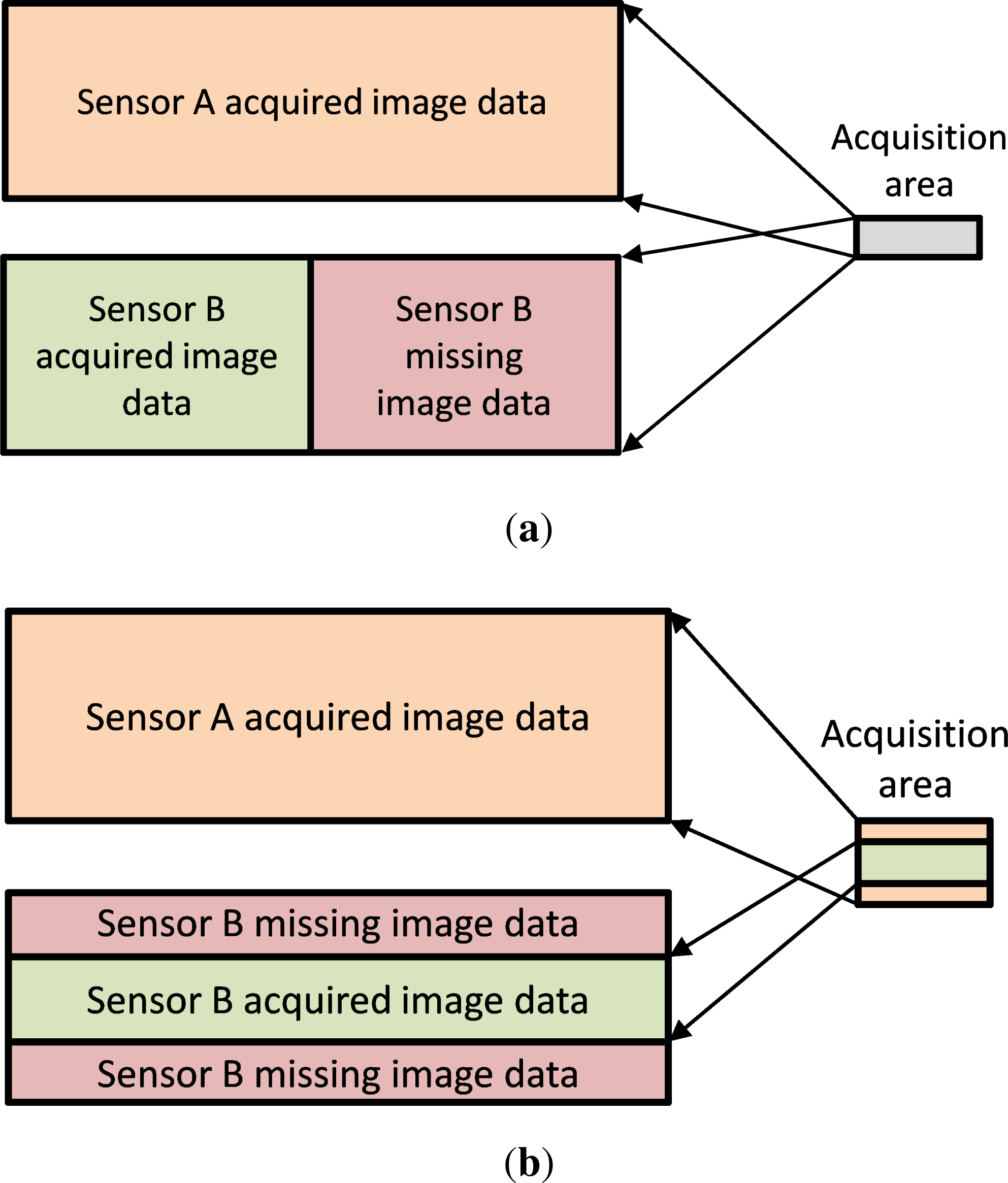
1.3. Missing Data Scenarios in This Study

Among the different missing data scenarios discussed above, we focus on two possible ones: sensor malfunctioning and differences in field of view (FOV). In the first scenario, two detectors or sensors with different spectral ranges acquire data on the same geographical area, but one of the sensors stops its image acquisition as a result of sensor malfunctioning. The result is that sensor A has full spatial image coverage of the area and sensor B has partial spatial image coverage, as illustrated in Figure 1a. With airborne data, if the malfunction is detected and can be repaired during the flight, it is possible to repeat the acquisition at an additional cost. Otherwise, the data of sensor B remains missing. The option of repeating the acquisition after repairing the sensor is not available for satellite platforms. In the second scenario, sensor A and sensor B have different FOVs, which result in a different acquisition swath. In that case, sensor A covers a wider area than sensor B, as illustrated in Figure 1b. An example of such a case with airborne data is the airborne imaging spectrometer for different applications (Aisa) with two types of sensors Aisa-Eagle and Aisa-Owl. The Aisa-Eagle can cover the VIS spectral range with a FOV of 35.5°, and the Aisa-Owl can cover the LWIR spectral range with a FOV of 24° [24]. The purpose of this study is therefore to develop a method that can make use of a VIS spectral range detector or sensor to predict an LWIR spectral range detector or sensor. In our case study, we use the AHS sensor, which incorporates both spectral range detectors.

1.4. Paper Outline

This paper is organized as follows. In Section 2, we describe the proposed sensor-to-sensor (SENTOS) prediction method, where one sensor is predicted using a different sensor and a learning dataset. Then, we describe the study area of Sokolov, Czech Republic, the AHS-acquired data and the datasets that were used in this study. In Section 3, we apply the SENTOS method to predict the LWIR spectral region using the VIS spectral region and evaluate the error of the predicted LWIR spectral image. In addition, we generate quartz and clay maps using the predicted LWIR spectral image and evaluate their performance using the receiver operating characteristic (ROC) curve. We conclude and suggest future work in Section 4.

2. Materials and Methods

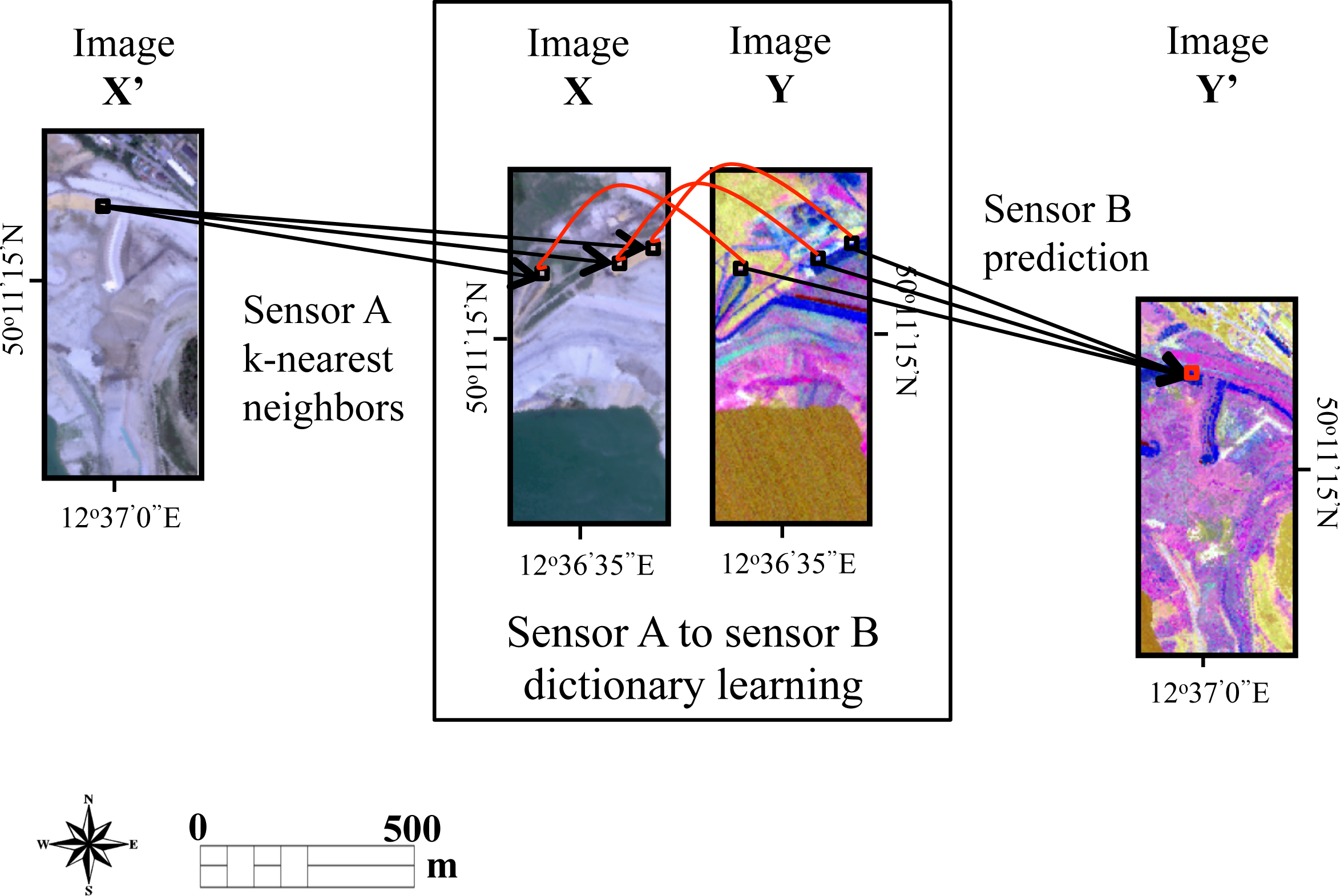
2.1. Sensor-to-Sensor Prediction (SENTOS) Method

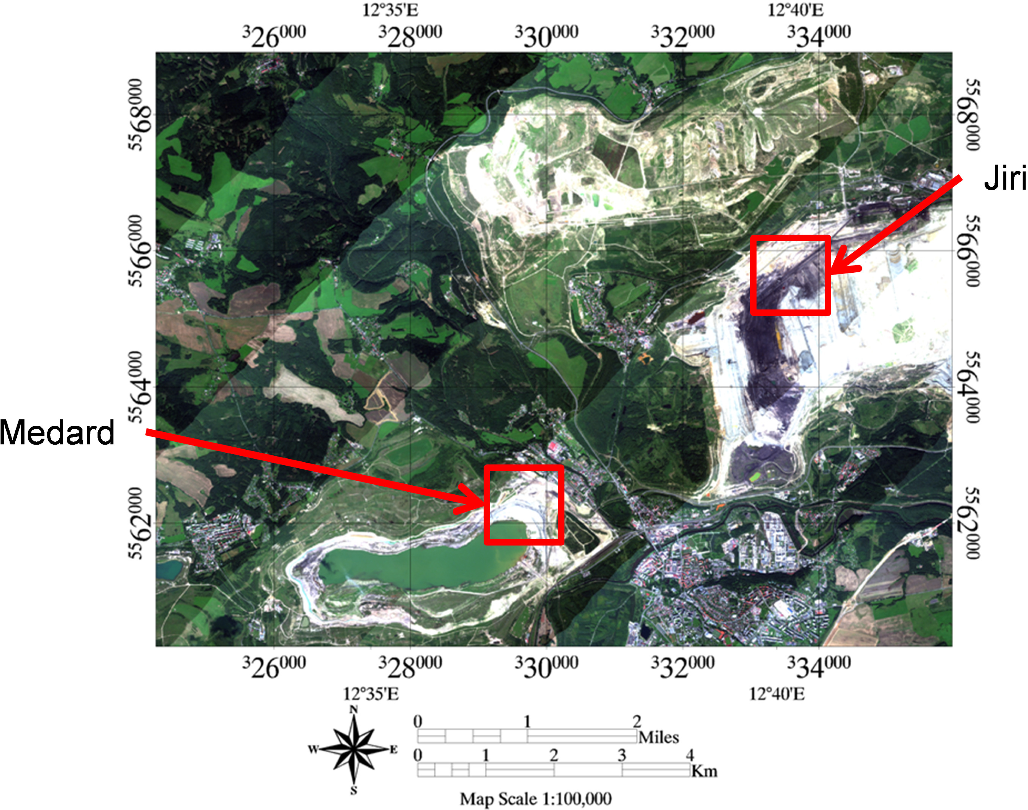
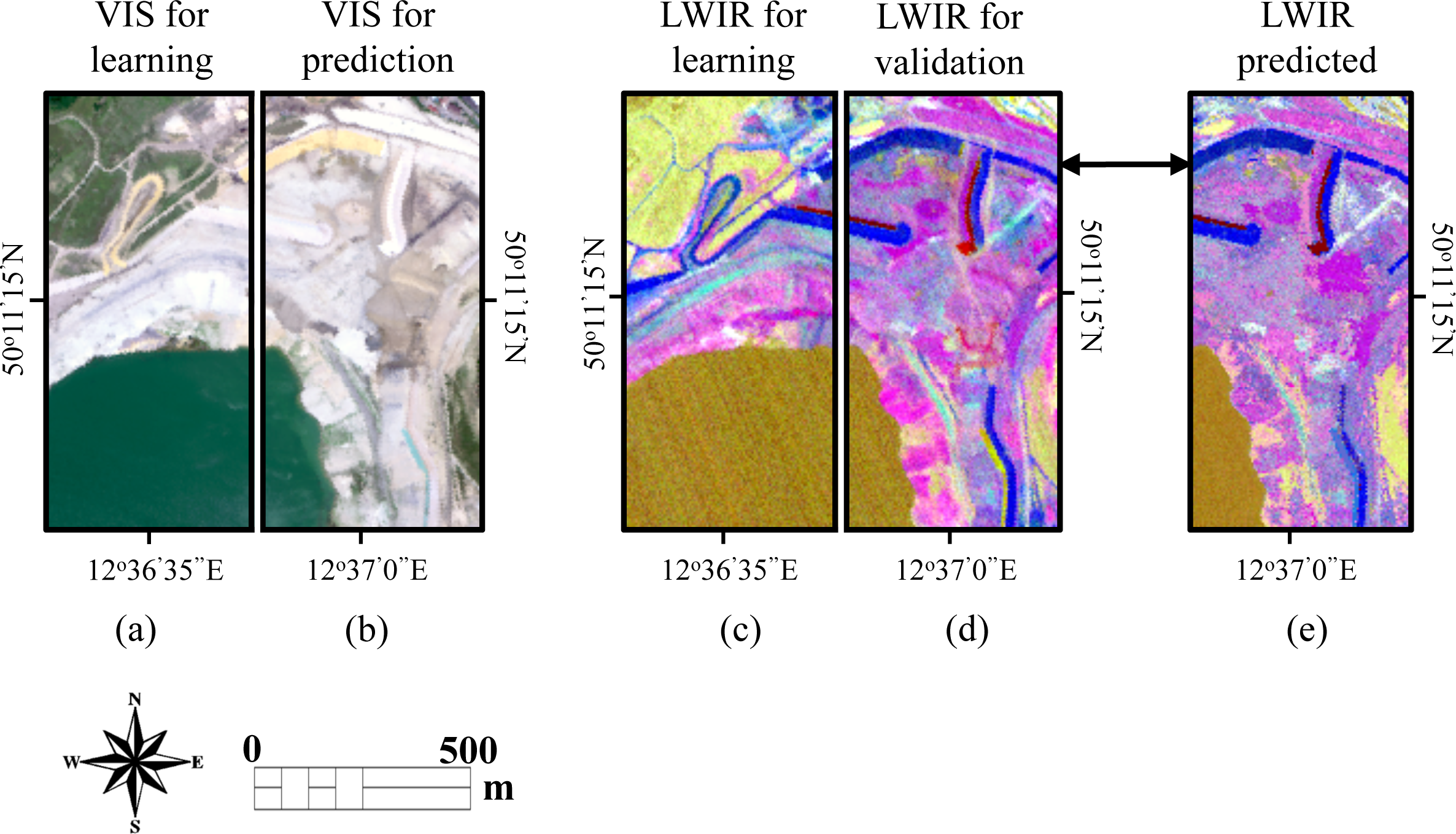
In this section, we describe the proposed method for predicting the spectral image of one sensor using the spectral image from a different type of sensor. The suggested method is based on the well-known k nearest-neighbors imputation procedure [11,25,26] that has been successfully demonstrated for missing data imputation in forestry remote sensing, where missing forest-related characteristics were imputed using the Landsat thematic mapper TMand ETM+ satellite image data [27–31] or airborne light detection and ranging LiDARimage data [32–34].

The VIS and LWIR detectors/sensors have distinct spectral behaviors for various targets (e.g., water, crops, soils, etc.). The proposed approach neither models the relationship by using a linear/nonlinear transformation nor does it claim that a physical relationship between the sensors exists. However, the proposed approach uses a “similarity assumption”, which suggests that same/similar materials will always retain corresponding reflectance (VIS) and emissivity (LWIR). Therefore, given a specific reflectance (VIS) spectra, the corresponding emissivity (LWIR) spectra can be deduced based on past measurements. In this study, we propose that if targets are measured by both VIS and LWIR detectors/sensors, those measurements can be stored in a collection that produces a “spectral dictionary”. This dictionary can, in turn, be used to extract a corresponding spectra following the similarity assumption. For example, if a target has a VIS spectrum that has a matching same/similar VIS spectrum in the spectral dictionary, we can use the corresponding LWIR spectrum from the spectral dictionary as a good/reasonable estimate for the LWIR spectra of the target in question. In this section, we use a general notation in which the VIS spectral range detector/sensor is denoted by sensor A and the LWIR spectral range detector/sensor is denoted by sensor B.

The proposed method has two main steps. In the first, we determine the relationship between sensor A’s spectral range and sensor B’s spectral range. We generate a spectral dictionary using pairs of geolocated pixels of both sensor A and sensor B detectors/sensors acquired at the same time (green areas in Figure 1). In the second step, a second sensor A spectral image subset (over a different geographical area marked in red in Figure 1 where the sensor B spectral image is missing) and the spectral dictionary (which was generated in the first stage) are used to predict the second sensor B spectral image subset (which was missing).

Consider an area imaged by both sensor A and sensor B. Assume that part of this areas was imaged by both sensors simultaneously and part by only sensor A. For the subset of the area that was imaged by both sensors A and B simultaneously, we denote the sensor A measurement of this area by X and its sensor B measurement by Y. The area for which a sensor A measurement exists without a sensor B measurement is denoted by X′, and its predicted sensor B image is denoted by Y′.

The subset images, $\mathbf{X}\triangleq \left\{{\mathbf{x}}_{\mathit{ij}}^{(p)}\right\}$ and $\mathbf{Y}\triangleq \left\{{\mathbf{y}}_{\mathit{ij}}^{(l)}\right\}$, will be used as a spectral dictionary and have the same spatial image dimensions, but a different number of bands, according to each of the sensors’ specifications where, i = 1 : N₁, j = 1 : M₁, p = 1 : P, l = 1 : L, i is the ith row, j is the jth column, p is the pth spectral band of X, l is the lth spectral band of Y, N₁ is the number of rows, M₁ is the number of columns and P and L are the number of spectral bands in images X and Y, respectively. In the same manner, ${\mathbf{X}}^{\prime }\triangleq \left\{{{\mathbf{x}}^{\prime }}_{\mathit{ij}}^{(p)}\right\}$ and ${\mathbf{Y}}^{\prime }\triangleq \left\{{{\mathbf{y}}^{\prime }}_{\mathit{ij}}^{(l)}\right\}$ have the same spatial image dimensions, where i = 1 : N₂, j = 1 : M₂, p = 1 : P, l = 1 : L, i is the ith row, j is the jth column, p is the pth spectral band of X, l is the lth spectral band of Y, N₁ is the number of rows, M₁ is the number of columns and P and L are the number of spectral bands in images X and Y, respectively. The spectral image, Y′, is our estimate of how the area of image X′ would look if it were acquired with sensor B.

The dimensions of the learning and predicted images are not necessarily the same and depend on the missing data scenario illustrated in Figure 1a,b. The dimensions of X and Y must be the same, as well as those of X′ and Y′. For example, if the data are missing due to a sensor malfunction, as illustrated in Figure 1a, then X and X′ will have the same number of rows, but not necessarily the same number of columns. On the other hand, if the missing data are a result of a different field of view as illustrated in Figure 1b, X and X′ will have the same number of columns, but not necessarily the same number of rows.

The relationship between sensors A and B is defined by their respective pixel locations. That is, since both spectral images were acquired over the same area, every pixel of sensor A’s spectral image has a corresponding geolocated pixel in sensor B’s spectral image. This defines the relationship between the two detectors/sensors, since the same material is captured with both. Therefore, if a sensor A pixel has a very similar pixel in the spectral dictionary, it is likely that its corresponding sensor B pixel (in the spectral dictionary) will be similar to a sensor B pixel, if such a pixel was acquired and was not missing.

To estimate Y′, we propose the following scheme. We search for the k nearest neighbors (k-NN) [25] of every pixel x′_ij in X under a distance metric, such as Euclidean, standardized Euclidean, Mahalanobis, cosine or correlation (described in Appendix A):

$$\left[I_{\mathit{ij}},{\mathbf{d}}_{\mathit{ij}}\right]=\mathit{knn}({{\mathbf{x}}^{\prime }}_{\mathit{ij}},\mathbf{X})\hspace{0.17em}\hspace{0.17em}\hspace{0.17em}\hspace{0.17em}\hspace{0.17em}\hspace{0.17em}\hspace{0.17em}\hspace{0.17em}\hspace{0.17em}\hspace{0.17em}\forall (i,j)$$

(1)

where I_ij is a k ×2 matrix consisting of the locations of the k pixels that are most similar to x′_ij under the chosen metric and d_ij is a k dimensional vector indicating the distance of each neighboring pixel to x′_ij. Then, we combine the information on the relationship between X and Y and the k nearest neighbors of each pixel of X′ in X to predict the desired spectral image Y′ as:

$${{\mathbf{y}}^{\prime }}_{\mathit{ij}}=\sum _{n=1}^k{\alpha }^{(n)}{\mathbf{y}}_{\mathit{rt}}$$

(2)

where $(r,t)=I_{\mathit{ij}}^{(n)}$ is the pixel location of the nth nearest neighbor (of x′_ij) in X and the weight of this nth nearest neighbor is given by [29]:

$${\alpha }^n=\frac{{\left(1/{\mathbf{d}}_{\mathit{ij}}^{(n)}\right)}^t}{{\sum }_{m=1}^k{\left(1/{\mathbf{d}}_{\mathit{ij}}^{(m)}\right)}^t}$$

(3)

The weight in Equation (3) is such that smaller distances are given higher importance in estimating Y′. This proposed method is illustrated in Figure 2 and the following pseudocode.

Algorithm 1:. SENTOS method pseudocode.

Algorithm 1:. SENTOS method pseudocode.

Naively, k nearest neighbors (kNN) computes the distance from a given pixel to all other pixels and selects the k ones with the smallest distance as the nearest neighbors. However, this operation in computationally expensive, and in practice, faster algorithms exist, for example, constructing a search tree on the space of pixels [35] or randomization-based search [36]. In this study, the search tree technique is used for finding the nearest neighbors. The VIS sensor/detector serves as sensor A, and the LWIR sensor/detector serves as sensor B.

2.2. Study Area

The Sokolov basin is located in northwestern Bohemia, Czech Republic. Its LULC consists of vegetation cover, bare soil, water bodies and man-made materials. It is characterized by large areas of vegetation cover, which include forests, agricultural areas, shrubs and grassland. It is largely affected by mining activities, such as open casts, dump sites, abandoned mines and acid mine drainage [37–39]. Its main mining activities include coal, kaolinite and granite extraction. The area is surrounded by cities, villages and agricultural areas, including the famous Karlovy Vary spa and springs. Recultivation activities in this area include planting pine trees in waste dumps and filling the open casts of closed mines with water, from either water pipes or shifted river streams.

2.2.1. Flight Acquisition, Sensor Description, Band Selection and Preprocessing

Airborne image acquisition was conducted on July 19, 2011 over the Sokolov area. The flight campaign included nine flight lines and one diagonal flight line. The airborne campaign was conducted in collaboration with the Spanish Aerospace Institute (INTA) using the AHS sensor [40] developed by Sensytech Inc. (Argon St. Inc., Beverly, MA, USA). The flight height was set to 1,839 m above ground level, acquiring imagery with a 90° FOV and 2.5 mrad instantaneous FOV, resulting in a spatial resolution of 4.6 m. The AHS sensor incorporates five detectors in the following manner: 20 bands in the range of 0.430–1.03 μm (VNIR, Si array detector), one band in the range of 1.55–1.75 μm (SWIR1, InSb array detector), 42 bands in the range of 2.0–2.54 μm (SWIR2, InSb array detector), seven bands in the range of 3.3–5.4 μm (mid wave infrared (MWIR), Mercury cadmium telluride (MCT) array detector) and 10 bands in the range of 8.20–12.70 μm (LWIR, MCT array detector). The bands in the SWIR (2.0–2.54 μm) region were very noisy, as were the bands in the near IR (0.826–1.03 μm). The first band in the VIS sensor (0.43 μm) was unusable. In this paper, we demonstrate the SENTOS method using the VIS range detector because of its widespread use on many airborne and satellite platforms. Therefore, 11 bands were selected for the VIS spectral image in the range of 0.5–0.796 μm, while the LWIR spectral image included nine bands in the range of 8.20–12.70 μm (LWIR region). The selected bands are summarized in

Table 1. The airborne hyperspectral scanner (AHS) sensor bands used in the VIS and LWIR spectral regions. Abbreviations: visible (VIS), long wave infra-red (LWIR), wavelength (WL), full-width half-maximum (FWHM)

Sensor	Band No.	Units	1	2	3	4	5	6	7	8	9	10	11
VIS	WL FWHM	[μm] [μm]	0.500 0.028	0.530 0.029	0.560 0.029	0.591 0.029	0.620 0.028	0.650 0.028	0.679 0.028	0.709 0.028	0.738 0.028	0.767 0.029	0.796 0.028
LWIR	WL FWHM	[μm] [μm]	8.310 0.458	8.770 0.421	9.237 0.424	9.680 0.455	10.143 0.412	10.624 0.556	11.230 0.552	11.796 0.566	12.371 0.543

. The 8-μm to 12-μm LWIR sensor has discriminative capabilities for quartz-composed minerals and clay minerals, which is important in this mining area. It can be used to monitor mining progress in the area as different layers of outcrops are revealed. Atmospheric correction for the VIS region was conducted with atmospheric correction now (ACORN) software [41], and emissivity in the LWIR spectral region was determined according to the temperature emissivity separation procedure [42]. Georectification of the AHS strips was performed with parametric geocoding and orthorectification for airborne optical scanner data (PARGE) software [43], and mosaicking of the rectified images was performed using environment for visualizing images (ENVI) software. The proposed approach and performance evaluation was implemented in Matlab by MathWorks Inc. (Natick, MA, USA).

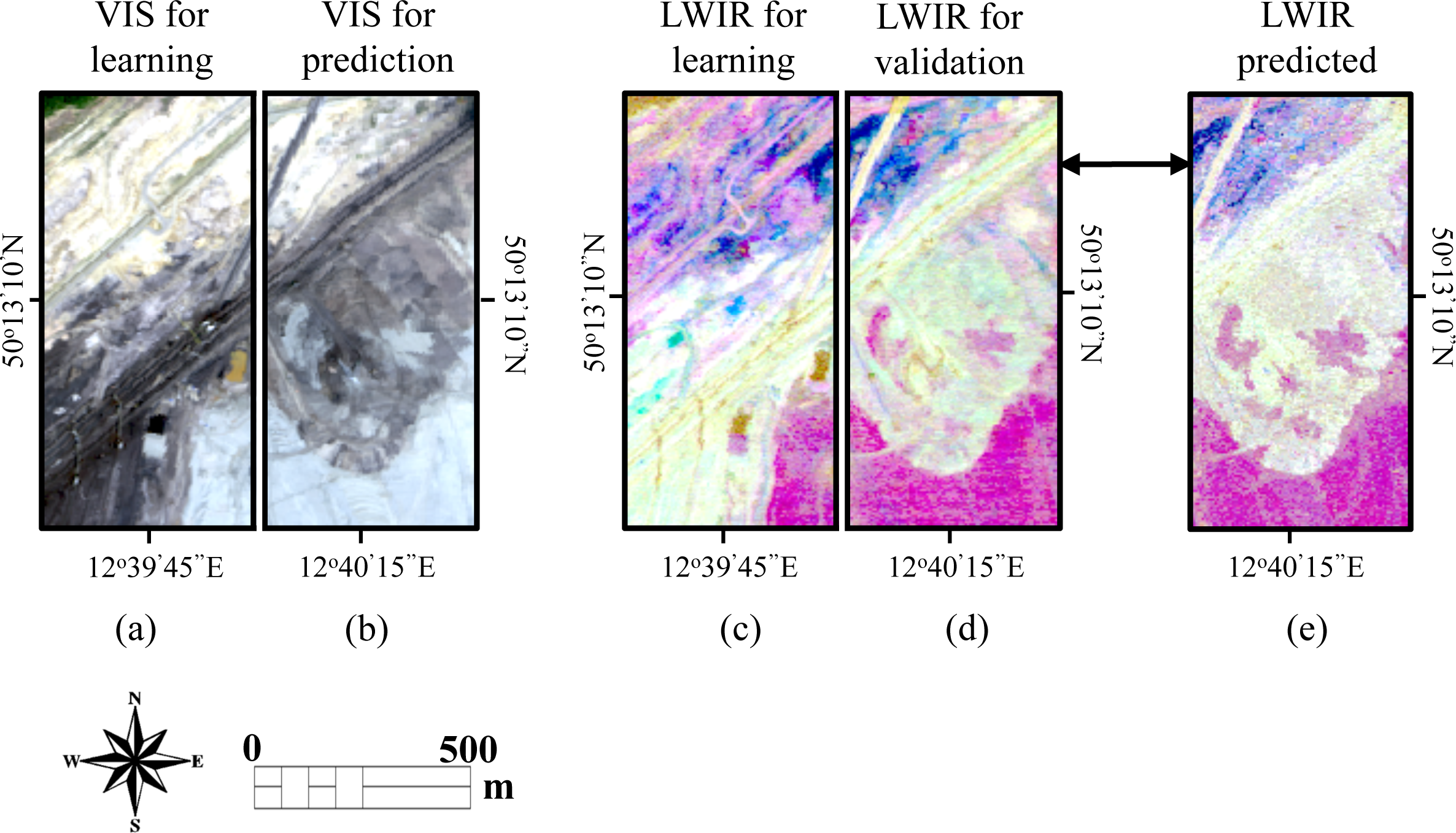
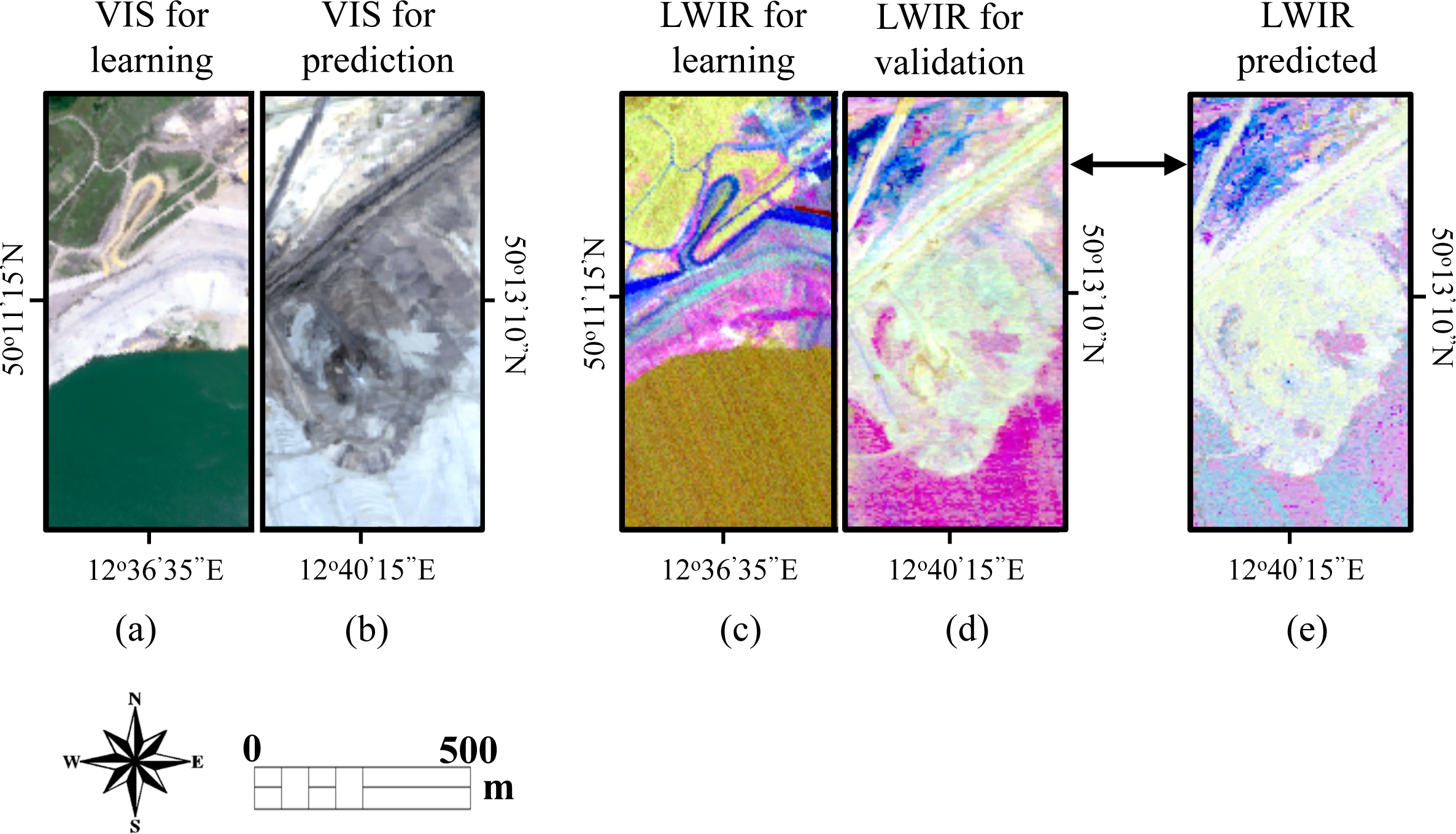
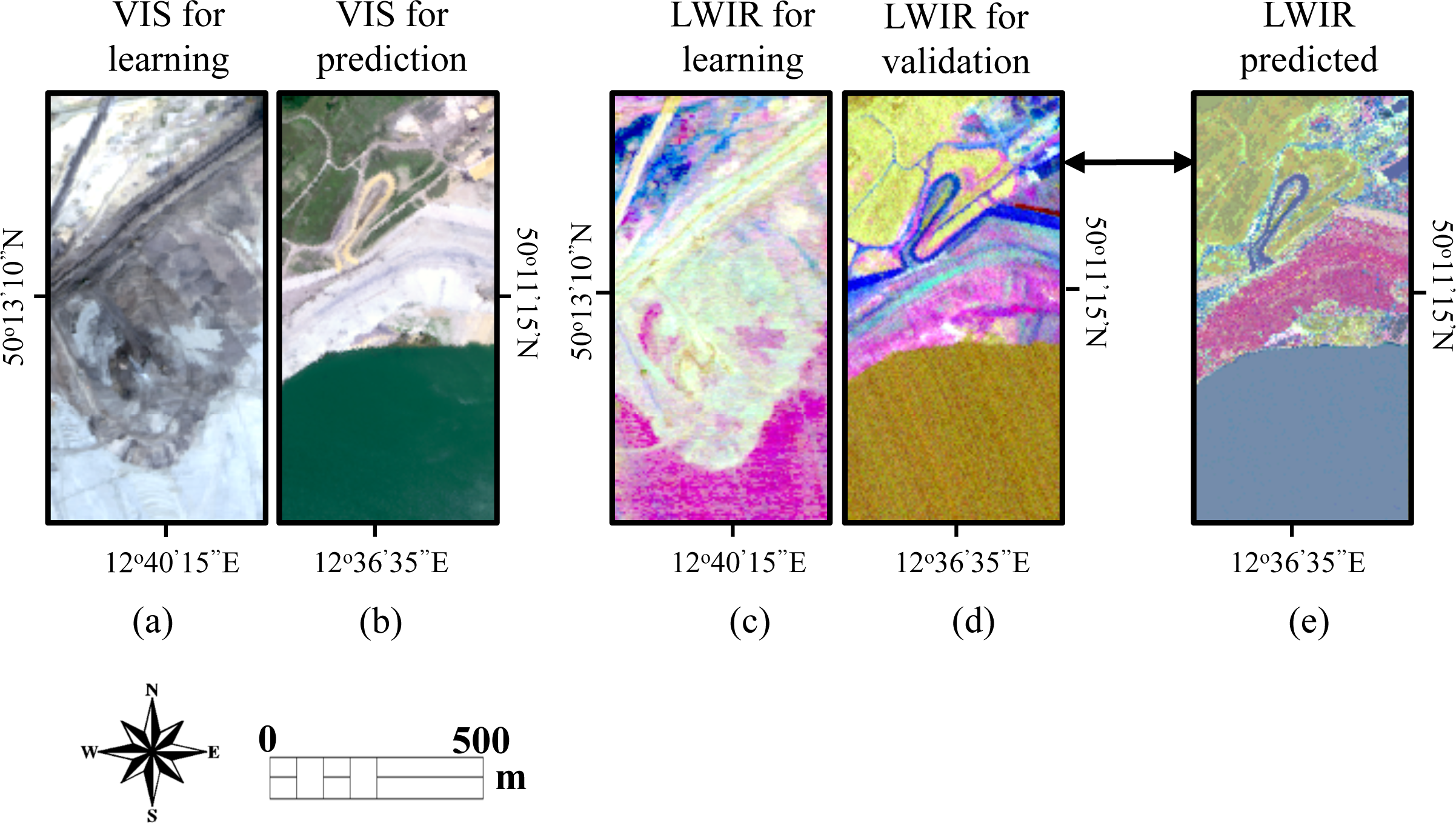
2.2.2. LWIR Prediction Schemes

Two subsets of the spectral image were selected to demonstrate the SENTOS prediction method, both subsets having quartz and clay minerals (Figure 3). The first subset, consisting of 200 rows and 200 columns, is located on the east side of Medard lake and includes the Medard abandoned coal mine. This area is characterized by different recultivation activities, such as filling the Medard open pit with water and the deposition of weathered granites transported from the Druzba opencast mine northeast of Sokolov, and natural outcrops of clays and claystones of the Cypris Formation [37]. The second subset, consisting of 200 rows and 200 columns, was selected over the Jiri active coal mine. This area mainly includes outcrops of clay minerals, coal and deposition of granites (quartz-rich minerals) from the Nove Sedlo formation. Using these two subregions of the input image, we generated four different experimental datasets, as shown in

Table 2. Experimental image dataset scheme.

Experiment Dataset No.	Medard Left	Medard Right	Jiri Left	Jiri Right
1	Learning	Predicted
2			Learning	Predicted
3	Learning			Predicted
4	Predicted			Learning

. The VIS and LWIR spectral images (of both the Medard and Jiri subsets) were divided into two equally-sized right and left images, with each image consisting of 200 rows and 100 columns. In all four datasets, we used a VIS spectral image to predict an LWIR spectral image. In the first dataset, we predicted the right side of the Medard image using its left side. In the second dataset, we predicted the right side of the Jiri image using its left side. In the third dataset, we predicted the right side of the Jiri image using the left side of the Medard image. In the fourth dataset, we predict the left side of the Medard image using the right side of the Jiri image.

3. Experimental Results

To evaluate the performance of the SENTOS prediction method, we calculated two performance measures. The first was the LWIR emissivity prediction error described in Section 3.1, where we calculate the difference between the predicted and real spectral emissivities. Simulations using different distance metrics and different numbers of nearest neighbors are shown to support the choice of k and the distance metric. The second performance measure, described in Section 3.2, evaluated the quartz and clay mineral mapping using the predicted LWIR emissivity image and compared the outcome to the quartz and clay maps obtained using the real LWIR emissivity image.

The LWIR and VNIR spectral regions exhibit complementary information with respect to the identification of minerals [44]. Therefore, it is important to validate the imputation of the missing LWIR data using thematic maps that incorporate the unique identification properties of the LWIR vs. VIS detectors/sensors. Such unique identification properties are known for quartz and clay minerals using the LWIR detector/sensor.

3.1. LWIR Spectral Image Prediction Error

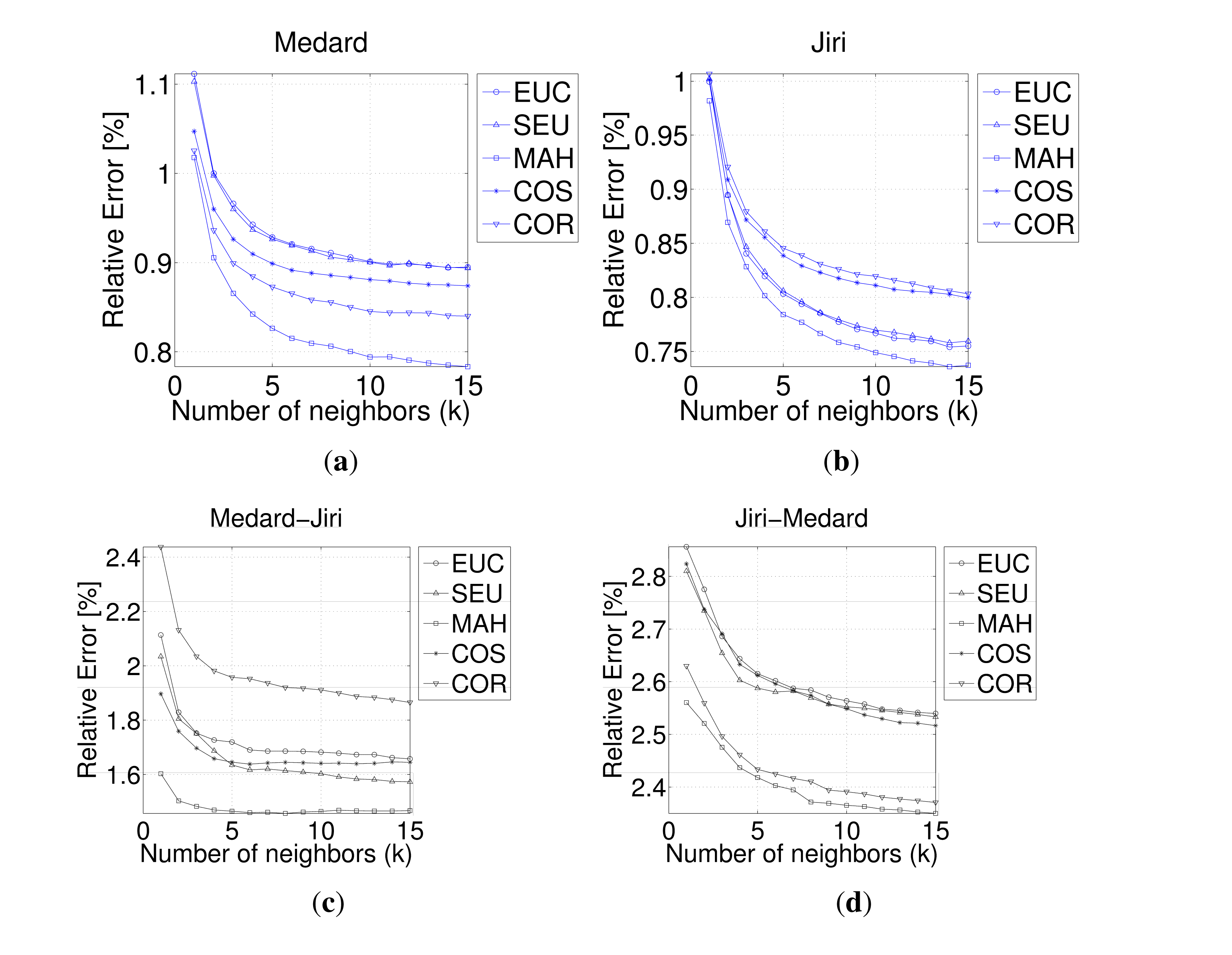
3.1.1. Tuning the kNN Algorithm

The kNN method described in Section 2.1 can be used with different numbers of nearest neighbors and different distance metrics. To choose the number of nearest neighbors (k), we calculated the relative error between the predicted and real emissivities as a function of k. This error is given by:

$${\mathbf{e}}_{\mathit{ij}}=\sqrt{\frac{{\sum }_{l=1}^L{\left({{\mathbf{y}}^{″}}_{\mathit{ij}}-{{\mathbf{y}}^{\prime }}_{\mathit{ij}}\right)}^2}{{\sum }_{l=1}^L{{\mathbf{y}}^{″}}_{\mathit{ij}}^2}}$$

(4)

where y″_ij is the real LWIR spectral image at the pixel location (i, j), which we use to validate the predicted spectral LWIR image, y′_ij.

This relative error was calculated for every pixel in each of the four experimental datasets described in Table 2. Hence, the calculation of this error for each dataset resulted in a distribution of relative error values. We used the median value of the relative error distribution to quantify the performance for each dataset, for various distance metrics and numbers of nearest neighbors (Figure 4). The lowest median relative error was achieved using the Mahalanobis distance for all four datasets (Figure 4). Focusing on the Mahalanobis distance, we observed a significant drop in the relative error of 18% and 16% when k was increased from one to five for the Medard and Jiri datasets, respectively. At over 10 nearest neighbors, the marginal decrease in the relative error was less than 0.5%. These results agree with previous findings indicating a low marginal improvement between 10 and 15 nearest neighbors [27,45,46]. Thus, we chose to use the kNN method with 10 nearest neighbors and the Mahalanobis distance metric to generate the thematic map in Section 3.2.

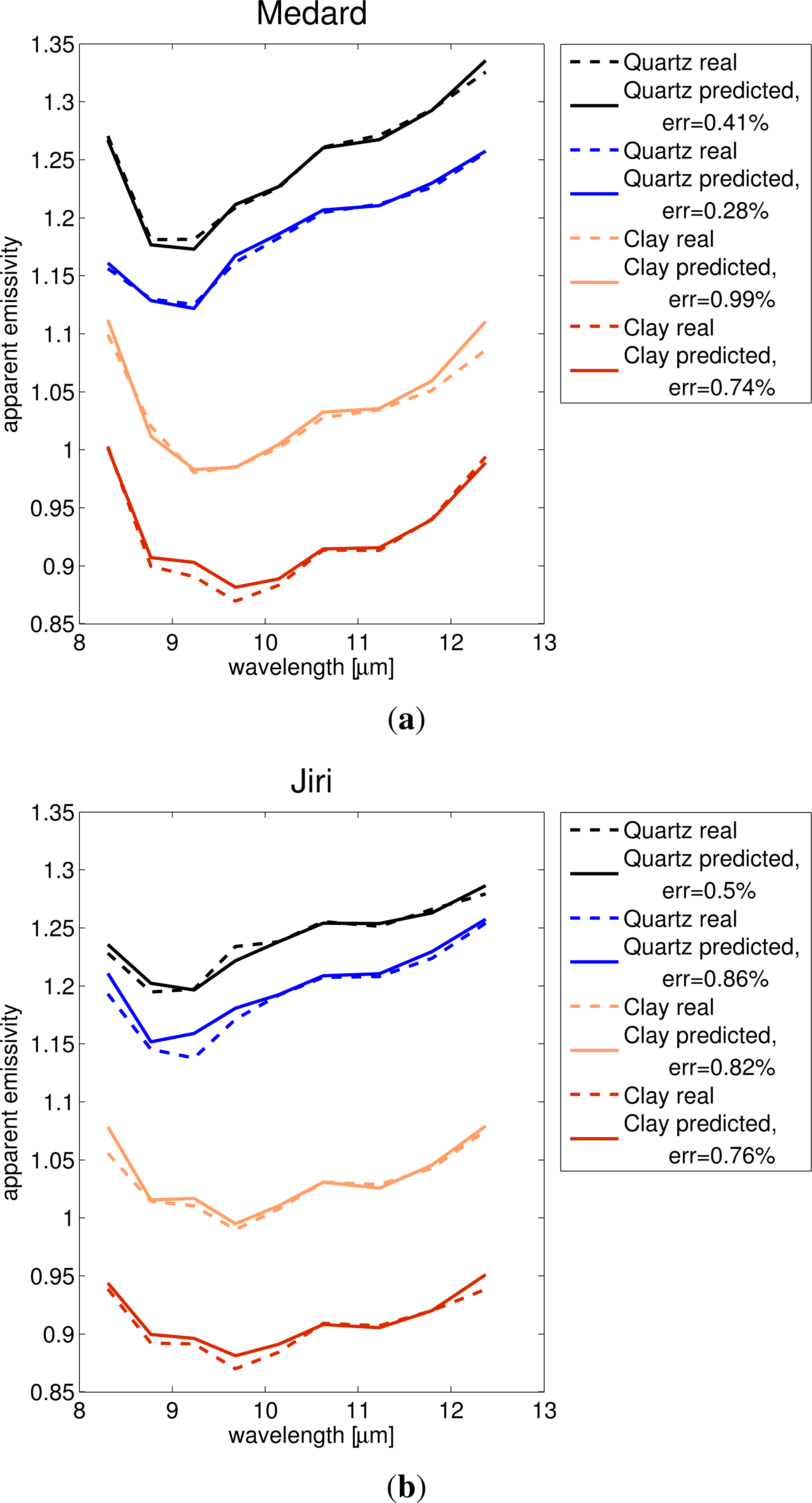
3.1.2. Examples of Predicted LWIR Spectra

Examples of predicted LWIR spectra for both the Medard and Jiri image subsets with the chosen kNN parameters (described in Section 3.1.1) are given in Figures 5a,b, respectively. The predicted emissivity spectra are indicated with solid lines and the real emissivity spectra with dashed lines. For each subset image, two example spectra are given for quartz minerals and two for clay minerals. In these examples, the predicted emissivity spectra gave a good estimation of the real emissivity spectra and low prediction errors of 0.28% and 0.41% for the quartz spectra and 0.74% and 0.99% for the clay spectra in the Medard image subset (Figure 5a).

Similar low prediction errors were achieved for the Jiri image subset, of 0.5% and 0.86% for the quartz spectra and 0.82% and 0.76% for the clay spectra (Figure 5b). These relative errors and spectra demonstrate that relative errors below 1% give similar emissivity spectra. The results in Figure 4 show that for the chosen kNN parameters (discussed in Section 3.1.1), median relative errors of 0.79% and 0.75% were achieved for the Medard and Jiri datasets. This indicates that most of the pixels were predicted with high accuracy, similar to the example spectra in Figure 5. Higher median relative errors of 1.46% and 2.37% were obtained with the Jiri-Medard and Medard-Jiri datasets, respectively, indicating a much lower prediction accuracy.

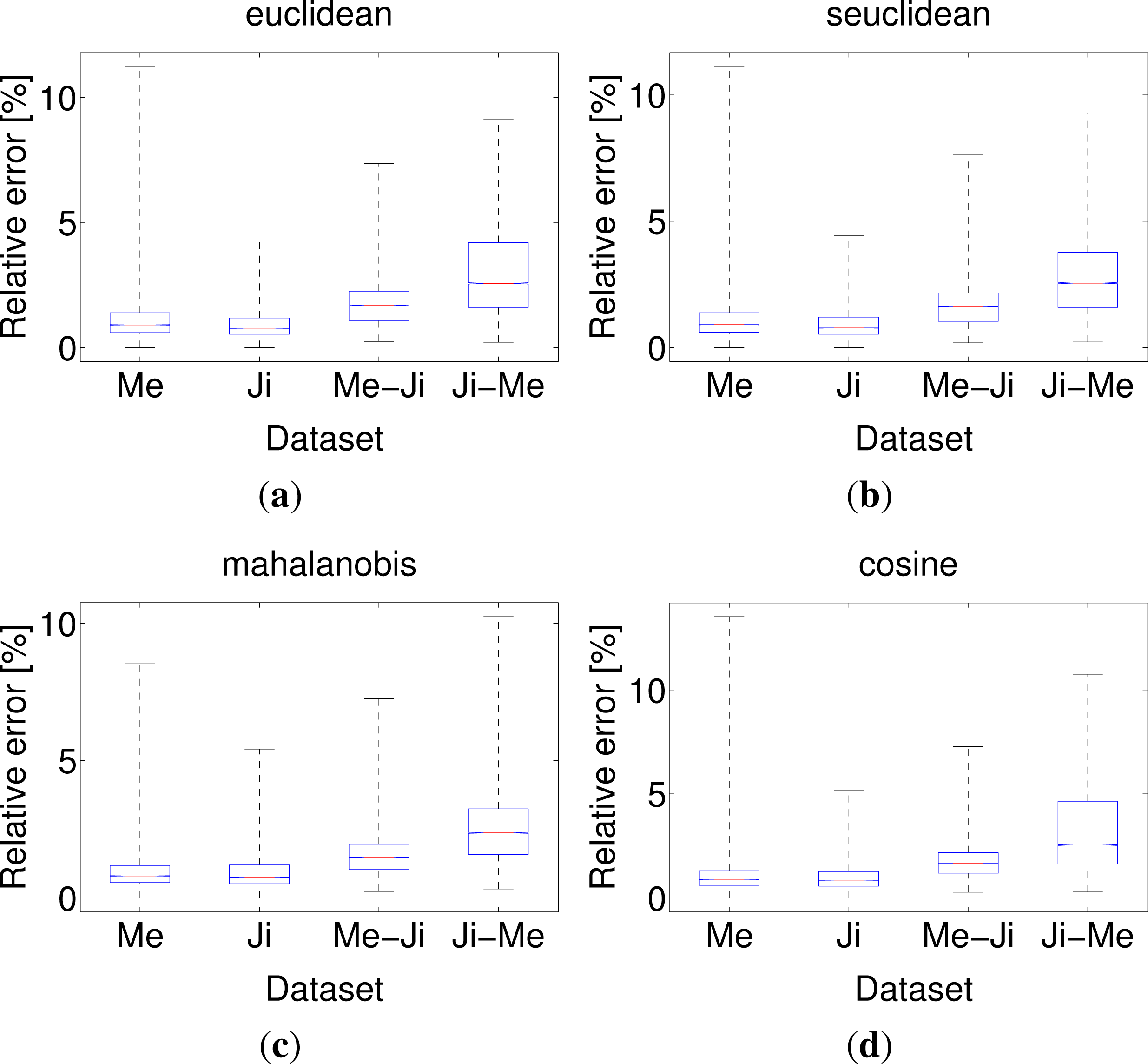
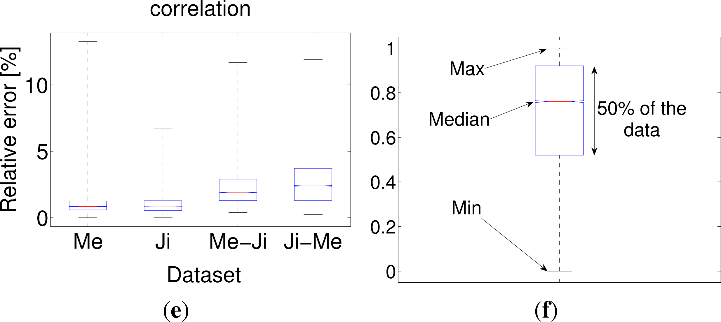
3.1.3. LWIR Prediction Error across the Different Datasets

Figure 4, which was discussed in Section 3.1.1, shows the median relative prediction error. In that figure, higher values were observed with the Medard-Jiri and Jiri-Medard datasets. However, a broader view of the distribution around the median values is missing. Thus, more detailed boxplot graphs are shown in Figure 6, presenting the distribution of the relative errors [47].

A boxplot graph is drawn for each of the four datasets used in this study (Me = Medard, Ji = Jiri); each graph has five marks: the median value of the error distribution, the minimum and maximum values and the 25th and 75th percentiles of the error distribution indicating 50% of the distribution around the median, as shown in the boxplot legend in Figure 6f. We show the results of the prediction error for the following metric distances: Euclidean, standardized Euclidean, Mahalanobis, cosine and correlation (the mathematical description is given in Appendix A), where each subfigure in Figure 6 represents a different distance metric. The Medard-Jiri and Jiri-Medard datasets exhibited wider distribution spreads and higher values of median relative error than the Medard or Jiri datasets. This means that the Medard-Jiri and Jiri-Medard datasets introduced lower prediction accuracies than the Medard and Jiri datasets.

The resulting predicted LWIR spectral images are shown next to the real LWIR spectral images and the learning VIS and LWIR spectral images in Figures 7, , and 10 for the Medard, Jiri, Medard-Jiri and Jiri-Medard datasets, respectively. The VIS spectral images are shown in true color composition, and the LWIR spectral images are shown in false color composition with band numbers 2, 4 and 8 (8.77 μm, 9.68 μm and 11.796 μm, respectively).

Each of Figures 7 and 10 is comprised of five subfigures according to the following: (a) VIS spectral image used in the learning stage; (b) VIS spectral image used to predict its corresponding LWIR spectral image; (c) LWIR spectral image used in the learning stage; (d) LWIR real spectral image used for validation and performance evaluation; and (e) predicted LWIR spectral image.

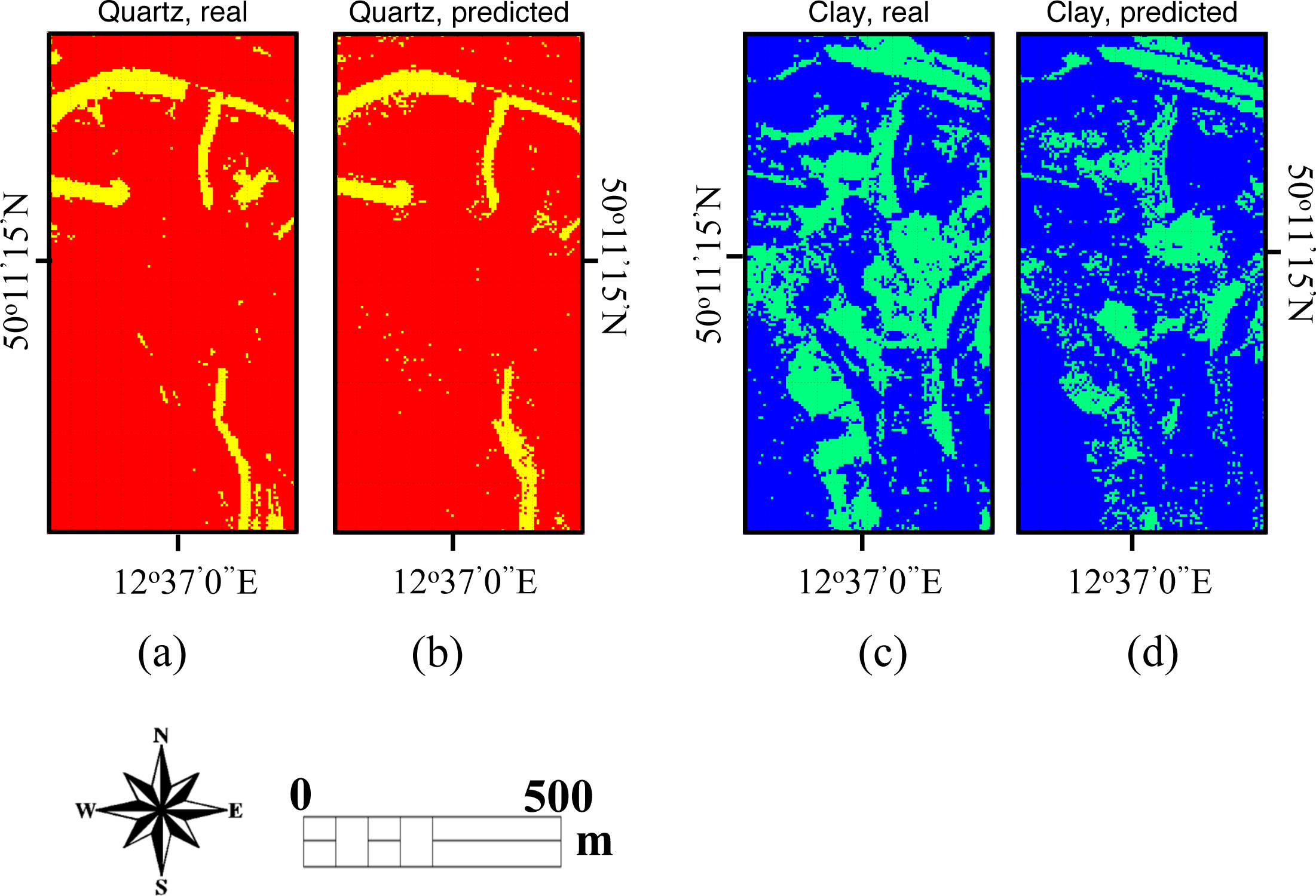
3.2. Predicting Quartz and Clay Mapping

In addition to the prediction error, we also evaluated the quartz and clay mineral mapping of the predicted LWIR spectral images. We produced quartz and clay mineral maps (Figures 11 and 14) from both real and predicted LWIR spectral images. The quartz and clay maps produced using the real LWIR spectral images were validated with a ground team survey according to the description in [37]. The quartz and clay maps were determined using the band ratio index based on their known absorption features in the LWIR spectral range [16,17] with the decision criteria given by:

$$S_{\mathit{ij}}=\{\begin{array}{ll}1\hfill & \text{if}\hspace{0.17em}{b}_{\mathit{ij}}^{(4)}/b_{\mathit{ij}}^{(2)}>1\hfill \\ 0\hfill & \text{if}\hspace{0.17em}{b}_{\mathit{ij}}^{(4)}/b_{\mathit{ij}}^{(2)}\le 1\hfill \end{array}$$

(5)

where S_ij is the binary quartz mapping in pixel location (i, j) and $b_{\mathit{ij}}^{(2)}$ and $b_{\mathit{ij}}^{(4)}$ are the emissivity values in pixel (i, j) in bands 2 (8.77 μm) and 4 (9.68 μm), respectively. Similarly, the clay mapping decision criteria are given by:

$$C_{\mathit{ij}}=\{\begin{array}{ll}1\hfill & \text{if}\hspace{0.17em}{b}_{\mathit{ij}}^{(4)}/b_{\mathit{ij}}^{(2)}<1\hfill \\ 0\hfill & \text{if}\hspace{0.17em}{b}_{\mathit{ij}}^{(4)}/b_{\mathit{ij}}^{(2)}\ge 1\hfill \end{array}$$

(6)

where C_ij is the binary clay mapping in pixel location, (i, j). Figure 11a,c shows the quartz and clay maps from the real LWIR spectral images, respectively. The predicted quartz and clay maps using the predicted LWIR spectral image are shown in Figure 11b,d, respectively.

We quantified the performance of the quartz and clay mapping (Figure 15) by using the popular receiver operating characteristic (ROC) curve [48] in which the probability of false alarm (P_fa) and probability of detection (P_d) are calculated for each metric distance and each dataset for both the quartz mapping (Figure 15a) and the clay mapping (Figure 15b). The probability of false alarms (P_fa) was calculated as the number of pixels that were mistakenly indicated as quartz/clay pixels divided by the total number of non-quartz/non-clay pixels (as determined from the LWIR-defined quartz/clay map). The probability of detection (P_d) was calculated by dividing the number of correctly identified quartz/clay pixels by the total number of quartz/clay pixels (as determined from the LWIR-defined quartz/clay map). Every marker in Figure 15 is characterized by a marker shape and color according to the following marker notation: Euclidean-circle, standardized Euclidean-upright triangle, Mahalanobis-square, cosine-asterisk, correlation-inverted triangle and the following color notation: Medard (Me) dataset, blue; Jiri (Ji) dataset, black; Medard-Jiri (Me-Ji) dataset, red; Jiri-Medard (Ji-Me) dataset, magenta.

Figure 15a shows the ROC curve for the quartz mapping. While this figure introduces low P_fa with all datasets and distance metrics, with the highest score of 0.12, the P_d has a wider range of values, from 0.1 to 0.8. The best performance for the Medard dataset (blue) was achieved with the Mahalanobis distance, with P_d = 0.71 and P_fa = 0.025. The Jiri dataset (black) introduces the highest scores of P_d = 0.38 and P_fa = 0.004 for the Mahalanobis distance and a similar P_d equaling 0.39, but twofold the P_fa = 0.008 for the cosine distance measure. This agrees with the superiority of the Mahalanobis distance described in Section 3.1. The Medard-Jiri dataset (red) shows a wide range of P_d, from 0.235 to 0.795, where the highest score was achieved with the standardized Euclidean distance and the lowest with the correlation distance. The Mahalanobis distance achieves a P_d of 0.61 for this dataset with P_fa = 0.018, compared to P_fa = 0.0326 with the standardized Euclidean. The Jiri-Medard dataset shows the lowest P_fa = 0.005 with P_d = 0.24 compared to the 14-fold higher P_fa = 0.071 for the best scoring P_d = 0.379, which was achieved with the Euclidean distance.

Figure 15b shows the ROC curve for the clay mapping. This figure introduces a low P_fa with all datasets and distance metrics, with the highest score of 0.19, while the P_d has a wider range of values, from 0.025 to 0.875. The Medard, Jiri and Jiri-Medard datasets showed the best performance with the Mahalanobis distance, with P_d and P_fa pairs of (0.49, 0.084), (0.87, 0.038) and (0.53, 0.1). The Mahalanobis distance gave very low P_d with a value of 0.08 and a low P_fa of 0.015, as well as using the Medard-Jiri dataset, while the highest P_d in this dataset was achieved with the correlation distance, yielding P_d = 0.8 and P_fa = 0.094.

In general, the Mahalanobis distance gave the best performance for quartz and clay mapping. This is in agreement with the relative error performance evaluation described in Section 3.1 and other research findings [49,50]. These quartz and clay maps are characterized by relatively low false-alarm rates, but a wide range of probability of detection capabilities, with better results being expected when the learning and predicted areas incorporate as many similar materials/LULC as possible.

3.3. Uncertainties, Errors and Accuracies

We demonstrated the proposed SENTOS method performance using qualitative and quantitative measures. The average relative error measure shows that an error of less than 0.8% is achieved when the spectral dictionary is taken from areas located close to the areas that are used for prediction. In cases where the areas used for prediction are located far from the areas used for spectral prediction, the average relative error becomes about 2.6%. Obviously, the prediction quality of the proposed method depends on the richness of the spectral dictionary. Only materials in the prediction area, which have corresponding similar materials in the spectral dictionary, will be predicted with high accuracy.

The same performance degradation is shown with the quartz and clay mapping results in Section 3.2, where the best combination of the probability of detection and false-alarm rate was achieved when the spectral dictionary was taken from areas located close to the areas that were used for prediction.

Another important factor that affects the prediction accuracies is the inaccuracy in atmospheric and geometric correction. These inaccuracies can cause pixels of similar materials to have different spectra and different materials to have very similar spectra (under the similarity metric used). Therefore, the corresponding reflectance spectra in the spectral dictionary will not represent the same material, and the estimated LWIR emissivity spectra will not match the real emissivity spectra.

Despite all these limitations of the proposed approach, the results indicate that when the spectral dictionary represents the prediction area well, the estimation will provide sufficient results.

4. Summary and Conclusions

In this paper, we introduced a new method to predict the emissivity of an LWIR spectral region using the reflectance from a VIS spectral region. The proposed method can be used for two main scenarios in which part of the LWIR data is missing. In both scenarios, the acquisition platform incorporates both VIS and LWIR spectral detectors/sensors. In the first scenario, the missing LWIR data is a result of sensor malfunctioning during the acquisition. In the second scenario, differences in FOV between the VIS and LWIR sensors (smaller FOV in the latter) result in missing data at the edges of the acquired area. The method is based on two stages. In the first stage, the two non-missing spectral images of the two detectors/sensors are used to determine the VIS-to-LWIR dictionary. In the second stage, the missing LWIR data are predicted using the kNN method, the existing VIS data and the VIS-to-LWIR dictionary from the first stage. Different properties of the kNN method were simulated, and the results indicated the lowest prediction error with the Mahalanobis distance and 10 nearest neighbors. Nevertheless, quartz and clay mineral thematic mapping using the predicted LWIR spectral image indicated that in some cases, other distance metrics demonstrate better performance than the Mahalanobis distance. This study demonstrated that it is possible to estimate missing data using a learning group that represents the missing data well, In our case study, the two spectral range detectors were incorporated on the same airborne platform. For future work on this subject, we suggest using the SENTOS approach to temporally impute low temporal LWIR spectral images with high temporal VIS spectral images in a manner similar to that used in methods, such as STARFM. Another interesting direction would be to improve accuracy by performing band selection/weighting according to the desired application (such as clay and quartz mapping). In addition, using the proposed method to estimate land surface temperature (LST) [51,52] with limited calibrated data combined with VIS and/or LWIR data might be valuable for studies of, for example, climate change, land-atmosphere energy exchange and the global hydrological cycle.

References

1. Cihlar, J.; Ly, H.; Li, Z.; Chen, J.; Pokrant, H.; Huang, F. Multitemporal, multichannel AVHRR data sets for land biosphere studies—Artifacts and corrections. Remote Sens. Environ 1997, 60, 35–57. [Google Scholar]
2. Roy, D.; Lewis, P.; Justice, C. Burned area mapping using multi-temporal moderate spatial resolution data-a bi-directional reflectance model-based expectation approach. Remote Sens. Environ 2002, 83, 263–286. [Google Scholar]
3. Jonsson, P.; Eklundh, L. Seasonality extraction by function fitting to time-series of satellite sensor data. IEEE Trans. Geosci. Remote Sens 2002, 40, 1824–1832. [Google Scholar]
4. Lunetta, R.S.; Knight, J.F.; Ediriwickrema, J.; Lyon, J.G.; Worthy, L.D. Land-cover change detection using multi-temporal MODIS NDVI data. Remote Sens. Environ 2006, 105, 142–154. [Google Scholar]
5. Gao, F.; Masek, J.; Schwaller, M.; Hall, F. On the blending of the Landsat and MODIS surface reflectance: Predicting daily Landsat surface reflectance. IEEE Trans. Geosci. Remote Sens 2006, 44, 2207–2218. [Google Scholar]
6. Baladrón, C.; Aguiar, J.M.; Calavia, L.; Carro, B.; Sánchez-Esguevillas, A.; Hernández, L. Performance study of the application of artificial neural networks to the completion and prediction of data retrieved by underwater sensors. Sensors 2012, 12, 1468–1481. [Google Scholar]
7. Karnieli, A.; Ben-Dor, E.; Bayarjargal, Y.; Lugasi, R. Radiometric saturation of Landsat-7 ETM+ data over the Negev Desert (Israel): Problems and solutions. Int. Appl. Earth Obs. Geoinf 2004, 5, 219–237. [Google Scholar]
8. Shen, H.; Zhang, L. A MAP-based algorithm for destriping and inpainting of remotely sensed images. IEEE Trans. Geosci. Remote Sens 2009, 47, 1492–1502. [Google Scholar]
9. Little, R.J.; Rubin, D.B. Statistical Analysis with Missing Data; Wiley: New York, NY, USA, 1987; Volume 539. [Google Scholar]
10. Bertalmio, M.; Sapiro, G.; Caselles, V.; Ballester, C. Image Inpainting. Proceedings of the 27th Annual Conference on Computer Graphics and Interactive Techniques (SIGGRAPH’00), New Orleans, LA, USA, 23–28 July 2000; pp. 417–424.
11. García-Laencina, P.J.; Sancho-Gómez, J.L.; Figueiras-Vidal, A.R. Pattern classification with missing data: A review. Neural Comput. Appl 2010, 19, 263–282. [Google Scholar]
12. Roy, D.P.; Ju, J.; Lewis, P.; Schaaf, C.; Gao, F.; Hansen, M.; Lindquist, E. Multi-temporal MODIS–Landsat data fusion for relative radiometric normalization, gap filling, and prediction of Landsat data. Remote Sens. Environ 2008, 112, 3112–3130. [Google Scholar]
13. Gao, F.; Masek, J.G.; Huang, C.; Wolfe, R.E. Building a consistent medium resolution satellite data set using moderate resolution imaging spectroradiometer products as reference. J. Appl. Remote Sens 2010, 4, 043526:1–043526:22. [Google Scholar]
14. Walker, J.; de Beurs, K.; Wynne, R.; Gao, F. Evaluation of Landsat and MODIS data fusion products for analysis of dryland forest phenology. Remote Sens. Environ 2012, 117, 381–393. [Google Scholar]
15. Shen, H.; Wu, P.; Liu, Y.; Ai, T.; Wang, Y.; Liu, X. A spatial and temporal reflectance fusion model considering sensor observation differences. Int. J. Remote Sens 2013, 34, 4367–4383. [Google Scholar]
16. Ramsey, M.S.; Christensen, P.R.; Lancaster, N.; Howard, D.A. Identification of sand sources and transport pathways at the Kelso Dunes, California, using thermal infrared remote sensing. Geol. Soc. Am. Bull 1999, 111, 646–662. [Google Scholar]
17. Vaughan, R.; Calvin, W.M.; Taranik, J.V. SEBASS hyperspectral thermal infrared data: Surface emissivity measurement and mineral mapping. Remote Sens. Environ 2003, 85, 48–63. [Google Scholar]
18. Eisele, A.; Lau, I.; Hewson, R.; Carter, D.; Wheaton, B.; Ong, C.; Cudahy, T.J.; Chabrillat, S.; Kaufmann, H. Applicability of the thermal infrared spectral region for the prediction of soil properties across semi-arid agricultural landscapes. Remote Sens 2012, 4, 3265–3286. [Google Scholar]
19. Liang, S. Quantitative Remote Sensing of Land Surfaces; John Wiley & Sons: Hoboken, NJ, USA, 2005. [Google Scholar]
20. Zhou, L.; Dickinson, R.E.; Ogawa, K.; Tian, Y.; Jin, M.; Schmugge, T.; Tsvetsinskaya, E. Relations between albedos and emissivities from MODIS and ASTER data over North African Desert. Geophys. Res. Lett. 2003. [Google Scholar] [CrossRef]
21. Stathopoulou, M.; Cartalis, C.; Petrakis, M. Integrating corine land cover data and landsat TM for surface emissivity definition: Application to the urban area of Athens, Greece. Int. J. Remote Sens 2007, 28, 3291–3304. [Google Scholar]
22. Roerink, G.; Su, Z.; Menenti, M. S-SEBI: A simple remote sensing algorithm to estimate the surface energy balance. Phys. Chem. Earth B 2000, 25, 147–157. [Google Scholar]
23. Courault, D.; Seguin, B.; Olioso, A. Review on estimation of evapotranspiration from remote sensing data: From empirical to numerical modeling approaches. Irrig. Drain. Syst 2005, 19, 223–249. [Google Scholar]
24. Specim AISA Airborne Hyperspectral Imaging Systems—Spectral Cameras. Available online: http://www.specim.fi/index.php/products/airborne (1 March 2013).
25. Cover, T.; Hart, P. Nearest neighbor pattern classification. IEEE Trans. Inf. Theory 1967, 13, 21–27. [Google Scholar]
26. García-Laencina, P.J.; Sancho-Gómez, J.-L.; Figueiras-Vidal, A.R. K nearest neighbors with mutual information for simultaneous classification and missing data imputation. Neurocomputing 2009, 72, 1483–1493. [Google Scholar]
27. Franco-Lopez, H.; Ek, A.R.; Bauer, M.E. Estimation and mapping of forest stand density, volume, and cover type using the k-nearest neighbors method. Remote Sens. Environ 2001, 77, 251–274. [Google Scholar]
28. Ohmann, J.L.; Gregory, M.J. Predictive mapping of forest composition and structure with direct gradient analysis and nearest-neighbor imputation in coastal Oregon, U.S.A. Can. J. For. Res 2002, 32, 725–741. [Google Scholar]
29. Haapanen, R.; Ek, A.R.; Bauer, M.E.; Finley, A.O. Delineation of forest/nonforest land use classes using nearest neighbor methods. Remote Sens. Environ 2004, 89, 265–271. [Google Scholar]
30. Hudak, A.T.; Crookston, N.L.; Evans, J.S.; Hall, D.E.; Falkowski, M.J. Nearest neighbor imputation of species-level, plot-scale forest structure attributes from LiDAR data. Remote Sens. Environ 2008, 112, 2232–2245. [Google Scholar]
31. Muinonen, E.; Parikka, H.; Pokharel, Y.; Shrestha, S.; Eerikäinen, K. Utilizing a multi-source forest inventory technique, MODIS data and Landsat TM images in the production of forest cover and volume maps for the Terai physiographic zone in Nepal. Remote Sens 2012, 4, 3920–3947. [Google Scholar]
32. Holopainen, M.; Haapanen, R.; Karjalainen, M.; Vastaranta, M.; Hyyppä, J.; Yu, X.; Tuominen, S.; Hyyppä, H. Comparing accuracy of airborne laser scanning and TerraSAR-X radar images in the estimation of plot-level forest variables. Remote Sens 2010, 2, 432–445. [Google Scholar]
33. Kankare, V.; Vastaranta, M.; Holopainen, M.; Räty, M.; Yu, X.; Hyyppä, J.; Hyyppä, H.; Alho, P.; Viitala, R. Retrieval of forest aboveground biomass and stem volume with airborne scanning LiDAR. Remote Sens 2013, 5, 2257–2274. [Google Scholar]
34. Lindberg, E.; Holmgren, J.; Olofsson, K.; Wallerman, J.; Olsson, H. Estimation of tree lists from airborne laser scanning using tree model clustering and k-MSN imputation. Remote Sens 2013, 5, 1932–1955. [Google Scholar]
35. Friedman, J.H.; Bentley, J.L.; Finkel, R.A. An algorithm for finding best matches in logarithmic expected time. ACM Trans. Math. Softw 1977, 3, 209–226. [Google Scholar]
36. Jones, P.W.; Osipov, A.; Rokhlin, V. A randomized approximate nearest neighbors algorithm. Appl. Computat. Harmon. A 2013, 34, 415–444. [Google Scholar]
37. Rojik, P. New stratigraphic subdivision of the Tertiary in the Sokolov Basin in Northwestern Bohemia. J. GEOsci 2004, 49, 173–185. [Google Scholar]
38. Murad, E.; Rojik, P. Iron mineralogy of mine-drainage precipitates as environmental indicators: Review of current concepts and a case study from the Sokolov Basin, Czech Republic. Clay Miner 2005, 40, 427–440. [Google Scholar]
39. Kopackova, V.; Chevrel, S.; Bourguignon, A.; Rojík, P. Application of high altitude and ground-based spectroradiometry to mapping hazardous low-pH material derived from the Sokolov open-pit mine. J. Map 2012, 8, 220–230. [Google Scholar]
40. Casal, G.; Sánchez-Carnero, N.; Domínguez-Gómez, J.A.; Kutser, T.; Freire, J. Assessment of AHS (Airborne Hyperspectral Scanner) sensor to map macroalgal communities on the Ría de vigo and Ría de Aldán coast (NW Spain). Mar. Biol 2012, 159, 1997–2013. [Google Scholar]
41. Green, R.O. Atmospheric Correction Now (ACORN); ImSpec LLC: Palmdale, CA, USA, 2001. [Google Scholar]
42. Gillespie, A.; Rokugawa, S.; Matsunaga, T.; Cothern, J.; Hook, S.; Kahle, A. A temperature and emissivity separation algorithm for Advanced Spaceborne Thermal Emission and Reflection Radiometer (ASTER) images. IEEE Trans. Geosci. Remote Sens 1998, 36, 1113–1126. [Google Scholar]
43. Schlapfer, D.; Schaepman, M.; Itten, K. PARGE: Parametric geocoding based on GCP-calibrated auxiliary data. Proc. SPIE 1998. [Google Scholar] [CrossRef]
44. Hapke, B. Theory of Reflectance and Emittance Spectroscopy; Cambridge University Press: Cambridge, UK, 2012. [Google Scholar]
45. Tokola, T.; Pitkanen, J.; Partinen, S.; Muinonen, E. Point accuracy of a non-parametric method in estimation of forest characteristics with different satellite materials. Int. J. Remote Sens 1996, 17, 2333–2351. [Google Scholar]
46. Nilsson, M. Estimation of Forest Variables Using Satellite Image Data and Airborne Lidar. 1997. [Google Scholar]
47. McGill, R.; Tukey, J.W.; Larsen, W.A. Variations of box plots. Am. Stat 1978, 32, 12–16. [Google Scholar]
48. Metz, C.E. Basic principles of ROC analysis. Semin. Nucl. Med 1978, 8, 283–298. [Google Scholar]
49. De Maesschalck, R.; Jouan-Rimbaud, D.; Massart, D. The Mahalanobis distance. Chemometr. Intell. Lab 2000, 50, 1–18. [Google Scholar]
50. Blitzer, J.; Weinberger, K.Q.; Saul, L.K. Distance metric learning for large margin nearest neighbor classification. Adv. Neural Inf. Process Syst 2005, 1473–1480. [Google Scholar]
51. Inamdar, A.K.; French, A.; Hook, S.; Vaughan, G.; Luckett, W. Land surface temperature retrieval at high spatial and temporal resolutions over the southwestern United States. J. Geophys. Res.:Atmos 2008, 113, 7–16. [Google Scholar]
52. Wu, P.; Shen, H.; Ai, T.; Liu, Y. Land-surface temperature retrieval at high spatial and temporal resolutions based on multi-sensor fusion. Int. J. Digital Earth 2013, 6, 1–21. [Google Scholar]
Appendix
A. Metric Distances
In this section, we describe the mathematical notations for the different metric distances used in this paper, where d(ij)(rt) is the distance between a pixel in the ith row and jth column to a pixel in the rth row and tth column.
Euclidean distance:
d ( ij ) ( rt ) 2 = ( x ij x rt ) ( x ij x rt )
Standardized Euclidean distance:
d ( ij ) ( rt ) 2 = ( x ij x rt ) V 1 ( x ij x rt )
where V is the variance diagonal matrix.
Mahalanobis distance:
d ( ij ) ( rt ) 2 = ( x ij x rt ) C 1 ( x ij x rt )
where C is the covariance matrix.
Cosine distance:
d ( ij ) ( rt ) 2 = 1 x ij x rt ( x ij x ij ) ( x rt x rt )
Correlation distance:
d ( ij ) ( rt ) 2 = 1 ( x ij x ¯ ) ( x rt x ˜ ) ( x ij x ¯ ) ( x ij x ¯ ) ( x rt x ˜ ) ( x rt x ˜ )
where = ∑ijxij and = ∑rtxrt.
Figure 1. Possible usage scenarios of the proposed approach. (a) Sensor malfunction; (b) sensor narrow field of view (FOV).
Remotesensing 05 05757f1
Figure 2. Sensor-to-sensor (SENTOS) prediction algorithm. Image Y′ is the predicted sensor B (long-wave infrared (LWIR)) spectral image using the sensor A (visible (VIS)) spectral image, X′. The nearest neighbors of every pixel in X′ are found in the sensor A (VIS) spectral image X. Each of those neighboring pixels has a corresponding sensor B (LWIR) spectral signature, and these are then used to generate the predicted sensor B (LWIR) image, Y′, by a weighted average.
Remotesensing 05 05757f2
Figure 3. Sokolov area. The Medard and Jiri subsets used in this study are marked with red rectangles.
Remotesensing 05 05757f3
Figure 4. Median values of the LWIR spectral image prediction error as a function of the number of k nearest neighbors (kNN). Every subplot represents a different dataset: (a) Medard; (b) Jiri; (c) Medard-Jiri; and (d) Jiri-Medard. Each of these subplots incorporates five different metric distances with the following abbreviations: Euclidean (EUC), standardized Euclidean (SEU), Mahalanobis (MAH), cosine (COS) and correlation (COR).
Remotesensing 05 05757f4
Figure 5. Example spectra of the predicted spectral emissivity compared to the real spectral emissivity (shown with offset for clarity). Solid lines indicate predicted emissivity, and dashed lines indicate real emissivity. Two example spectra are given for quartz minerals and two for clay minerals. (a) Spectral emissivity examples from Medard dataset; (b) spectral emissivity examples from Jiri dataset. The relative error between the predicted and real emissivities is indicated in the legend.
Remotesensing 05 05757f5
Figure 6. Boxplot graphs of the error distribution calculated between the predicted and real LWIR spectral images. Each subplot represents the error associated with the following nearest-neighbor metrics: (a) Euclidean; (b) standardized Euclidean; (c) Mahalanobis; (d) cosine; (e) correlation; and (f) general descriptive boxplot graph. Every subplot has four boxplots, each one related to a different dataset with the following abbreviations: Me = Medard, Ji = Jiri, Me-Ji = Medard-Jiri and Ji-Me = Jiri-Medard.
Remotesensing 05 05757f6aRemotesensing 05 05757f6b
Figure 7. VIS and LWIR spectral images of the Medard dataset (VIS images are shown with true color composition, and LWIR images are shown with false color composition with bands 2,4 and 8 (8.77 μm, 9.68 μm and 11.796 μm, respectively)). (a) Original VIS spectral image used for the learning stage; (b) original VIS spectral image of the area to be predicted in the LWIR spectral image; (c) original LWIR spectral image used for the learning stage; (d) original LWIR spectral image of the predicted area (used to validate the results); (e) predicted LWIR spectral image.
Remotesensing 05 05757f7
Figure 8. VIS and LWIR spectral images of the Jiri dataset (VIS images are shown with true color composition, and LWIR images are shown with false color composition with bands 2,4,8 (8.77 μm, 9.68 μm and 11.796 μm, respectively)). (a) Original VIS spectral image used for the learning stage; (b) original VIS spectral image of the area to be predicted in the LWIR spectral image; (c) original LWIR spectral image used for the learning stage; (d) original LWIR spectral image of the predicted area (used to validate the results); (e) predicted LWIR spectral image.
Remotesensing 05 05757f8
Figure 9. VIS and LWIR spectral images of the Medard-Jiri dataset (VIS images are shown with true color composition, and LWIR images are shown with false color composition with bands 2,4,8 (8.77 μm, 9.68 μm and 11.796 μm, respectively)). (a) Original VIS spectral image used for the learning stage; (b) original VIS spectral image of the area to be predicted in the LWIR spectral image; (c) original LWIR spectral image used for the learning stage; (d) original LWIR spectral image of the predicted area (used to validate the results); (e) predicted LWIR spectral image.
Remotesensing 05 05757f9
Figure 10. VIS and LWIR spectral images of the Jiri-Medard dataset (VIS images are shown with true color composition, and LWIR images are shown with false color composition with bands 2,4,8 (8.77 μm, 9.68 μm and 11.796 μm, respectively)). (a) Original VIS spectral image used for the learning stage; (b) original VIS spectral image of the area to be predicted in the LWIR spectral image; (c) original LWIR spectral image used for the learning stage; (d) original LWIR spectral image of the predicted area (used to validate the results); (e) predicted LWIR spectral image.
Remotesensing 05 05757f10
Figure 11. Medard dataset, quartz and clay mapping of predicted and real LWIR spectral images. (a) Quartz mapping of original LWIR spectral image; (b) quartz mapping of predicted LWIR spectral image; (c) clay mapping of original LWIR spectral image; (d) clay mapping of predicted LWIR spectral image.
Remotesensing 05 05757f11
Figure 12. Jiri dataset, quartz and clay mapping of predicted and real LWIR spectral images. (a) Quartz mapping of original LWIR spectral image; (b) quartz mapping of predicted LWIR spectral image; (c) clay mapping of original LWIR spectral image; (d) clay mapping of predicted LWIR spectral image.
Remotesensing 05 05757f12
Figure 13. Medard-Jiri dataset, quartz and clay mapping of predicted and real LWIR spectral images. Jiri coal mine area quartz and clay mapping using the Medard area as the learning image. (a) Quartz mapping of original LWIR spectral image; (b) quartz mapping of the predicted LWIR spectral image; (c) clay mapping of the original LWIR spectral image; (d) clay mapping of the predicted LWIR spectral image.
Remotesensing 05 05757f13
Figure 14. Jiri-Medard dataset, quartz and clay mapping of predicted and real LWIR spectral images. Medard lake area quartz and clay mapping using the Jiri coal mine area as the learning image. (a) Quartz mapping of the original LWIR spectral image; (b) quartz mapping of the predicted LWIR spectral image; (c) clay mapping of the original LWIR spectral image; (d) clay mapping of the predicted LWIR spectral image.
Remotesensing 05 05757f14
Figure 15. Receiver operating characteristic (ROC) curves. (a) ROC curve of quartz mapping; (b) ROC curve of clay mapping. Each dataset is represented by a different color as follows: Medard (Me), blue; Jiri (Ji), black; Medard-Jiri (Me-Ji), red; Jiri-Medard (Ji-Me), magenta. The distance metrics are abbreviated as: Euclidean (EUC), standardized Euclidean (SEU), Mahalanobis (MAH), cosine (COS) and correlation (COR). Better performance was achieved for the Medard (blue) and Jiri (black) datasets, since the predicted area is more similar to the learning area. The Medard-Jiri (red) and Jiri-Medard (magenta) learning areas are not similar enough to the predicted area and, therefore, achieve inferior performance.
Remotesensing 05 05757f15