Examining the Satellite-Detected Urban Land Use Spatial Patterns Using Multidimensional Fractal Dimension Indices

Abstract

Understanding the spatial patterns of urban land use at both the macro and the micro levels is a central issue in global change studies. Due to the nonlinear features associated with land use spatial patterns, it is currently necessary to provide some distinct analysis methods to analyze them across a range of remote sensing imagery resolutions. The objective of our study is to quantify urban land use patterns from various perspectives using multidimensional fractal methods. Three commonly used fractal dimensions, i.e., the boundary dimension, the radius dimension, and the information entropy dimension, are introduced as the typical indices to examine the complexity, centrality and balance of land use spatial patterns, respectively. Moreover, a new lacunarity dimension for describing the degree of self-organization of urban land use at the macro level is presented. A cloud-free Landsat ETM+ image acquired on 17 September 2010 was used to extract land use information in Wuhan, China. The results show that there are significant linear relationships represented by good statistical fitness related to these four indices. The results indicate that rapid urbanization has substantially affected the urban landscape pattern, and different land use types show different spatial patterns in response. This analysis reveals that multiple fractal/nonfractal indices provides a more comprehensive understanding of the spatial heterogeneity of urban land use spatial patterns than any single fractal dimension index. These findings can help us to gain deeper insight into the complex spatial patterns of urban land use.

1. Introduction

Land use and cover change (LUCC) is one of the most profound human-induced alterations to the Earth’s surface [1–6]. Numerous studies have shown that remote sensing satellite imagery is the major data source for analyzing the spatial patterns of urban land use [7–13]. The availability of land use spatio-temporal information derived from multi-resolution images of remote sensing satellites, such as Landsat, National Oceanic and Atmospheric Administration (NOAA), Moderate resolution Imaging Spectroradiometer (MODIS), and Satellite pour l’Observation de la Terre (SPOT), has significantly facilitated the study of urban land use spatial structure [14,15]. Therefore, it is very important to provide some distinct analysis methods to characterize spatial patterns across a range of remote sensing imagery resolutions in land use studies.

Remote sensing images can objectively and truthfully record the phenomena of the Earth’s surface. As remote sensing satellites have provided more abundant land use information in the past ten years than at any other time in history, the analysis of satellite-detected urban land use has been recognized as the current mainstream approach to studying urban spatial patterns [16,17]. For various remote sensors with different spatial resolutions, there are many case studies regarding the application of satellite-based remote sensing imagery that have demonstrated its good performance in assessing the spatial patterns of land use since 2000. In the early 21st century, Foody mapped land cover from an airborne thematic mapper (ATM) sensor with a neural network classification [18]. Kalluri et al. attempted to examine land cover dynamics based on Landsat Thematic Mapper (TM) using high-performance computing algorithms [19]. Tadesse et al. combined Landsat TM and geographic information system technology to detect the land use change in Addis Ababa [20]. Friedl et al. presented algorithms to map global land cover from MODIS [21], while Huete et al. analyzed land cover conversion and land degradation from Earth Observing 1 (EO-1) Hyperion hyperspectral data [22]. Gitas et al. used NOAA-AVHRR imagery to map burned areas in Spain [23]. Thenkabail et al. utilized continuous streams of MODIS data to study the Ganges and Indus river basin land use/land cover [24]. De Almeida et al. used GIS to simulate the changes in urban land use from MSS and Landsat TM [25]. Duran et al. focused on acquiring and analyzing data on land use distribution in Istanbul by using GIS and remote sensing technology [26]. Recently, Chang and Tang used Landsat remote sensing images to assess the land use change after the Northridge Earthquake [27]. Zurita-Milla et al. used medium spatial resolution satellite images for land cover mapping [28], while Myint et al. extracted urban land cover information from high spatial resolution imagery [29], and Dymond et al. used SPOT 5 satellite imagery to explore the land use change in New Zealand [30]. In the past and at present, even in the future, remote sensing will likely always be the most important tool for studying land use and cover change.

Urban land use patterns involve not only single patch features at the micro level but also the overall spatial distribution at the macro level. The local spatio-temporal changes at the micro level often generate larger-scale emergent patterns of land use, which are in turn affected and restricted by land use spatial structure at the macro level [31,32]. According to different scales of land use spatial patterns, the micro characteristics at the patch level are usually defined by the boundary complexity (i.e., the geometric complexity of the shape), while the macro spatial distribution mainly refers to specific overall features, such as balance, centrality, and self-organization. The micro characteristics can be measured through the complexity and randomness of single land use patches, which have been thoroughly elaborated by previous studies [33,34]. For characteristics at different levels, however, the macro is considerably more complicated than the micro [35]. For instance, the centrality describes the radial spatial distribution and variation around only one designated center. Conversely, the self-organization expresses the aggregation tendency around multiple cluster centers. Furthermore, the balance describes the spatial aggregation degree in all directions, whose distribution probability is assumed to be equal, as if no aggregation center exists. In terms of the statistical theory, previous studies have attributed distinctively nonlinear features to these four land use spatial patterns as discussed above. Schmit (2006) and Kwan (2008) have also noted that the modifiable areal unit problem (MAUP), affected by geographical scale, exists in the analysis of land use, which easily leads to a serious statistical bias that can radically affect the results of statistical hypothesis tests [36,37]. That is, these four land use spatial patterns cannot be well quantified using statistical analysis methods [38,39].

Fractal dimensions have been used for their potential to measure the nonlinear characteristics associated with the spatial patterns of urban land use derived from remote-sensing imagery. Both self-similarity and randomness are two basic characteristics of fractals. It has been demonstrated that fractal dimensions are suitable for modeling the spatial distribution of many geographic phenomena on the earth [40]. The foundational work on the complexity analysis of satellite-detected land use spatial patterns using fractal dimensions was reported by De Cola [41] and Lam [42–49]. Nevertheless, it was not until the development of high-resolution remote sensing imagery in the past ten years that those classic fractal dimensions with the divider method originally developed by Goodchild and Shelberg were gradually extended to more research fields and that these fractal dimensions began to be more widely applied [50]. Emerson et al. utilized a fractal dimension to aid in multispectral image classification, which was particularly effective in resolving land cover classes within urbanized areas [51]. Tang et al. applied the area-weighted mean patch fractal dimension, together with the core area percentage of landscape and the area-weighted centroid method, to simultaneously estimate the forest spatial movement and the spatial fragmentation process [52]. Tran et al. explored the use of fractal dimensions to identify the homogeneity/heterogeneity thresholds of urban structure. It was found that the fractal theory-based index was more robust and transferable to discriminate among urban contexts than the local variance method [53]. Based on the land use information derived from eight satellite images of Indianapolis, USA taken by five remote sensors, Liang et al. evaluated the efficiency of three fractal algorithms (isarithm, triangular prism, and variogram) for describing urban landscapes [54]. The aforementioned studies show that fractal dimensions can describe the non-linear characteristics of urban land use patterns and have the potential to examine the inherent regularity, hierarchy and scale invariance of urban land use spatial patterns [55,56]. Despite these significant contributions of fractal dimensions to land use spatial pattern analysis, no substantial research has yet attempted to simultaneously use multiple fractal dimension indices to thoroughly examine land use spatial patterns. After all, the function of any single fractal dimension that quantifies land use spatial patterns from a certain perspective is too limited.

As summarized by Ling, there are currently three fractal dimensions for measuring land use spatial characteristics: the boundary dimension, the radius dimension and the information entropy dimension [38]. The boundary dimension (shown in Figure 1a) is used to express the complexity and randomness of land use patches [57,58], and the radius dimension (shown in Figure 1b) is used to quantitatively describe the centrality of land use patches [59,60]. The information entropy dimension shown in Figure 1c is applied to reveal the balance of the land use spatial distribution [61–63]. In addition, we propose the lacunarity dimension to describe the self-organization spatial pattern of land use, which has been seriously ignored in the literature. As is well known, urban areas mainly appear to have a single centrality in the initial development stage. Due to the uncontrollable expansion associated with rapid urbanization, its spatial heterogeneity gradually increases and results in an unbalanced situation with many centers. For instance, there are strong residential zoning tendencies to use extra land as open space and recreation in some metropolitan cities of China as well as America. Although this type of zoning land use pattern protects land for communities and to an extent preserves land from development, it is what ultimately leads to the suburban sprawl with the self-organization features shown in Figure 1d. For this emerging spatial pattern of land use, however, there is no corresponding fractal dimension index that could achieve a more comprehensive understanding of land use spatial characteristics and rules of urbanization process.

The main objective of this paper is to quantify the nonlinear spatial patterns of urban land use through multidimensional indices and to assess the single patch features at the micro level as well as the overall spatial distributions at the macro level. In particular, a new lacunarity dimension is proposed to describe the degree of self-organization with multiple centers, which cannot be examined by the three commonly used fractal dimensions (i.e., the boundary dimension, the radius dimension and the information entropy dimension). It is beneficial for us to create a more comprehensive understanding of the spatial heterogeneity of urban land use spatial patterns.

2. Methods

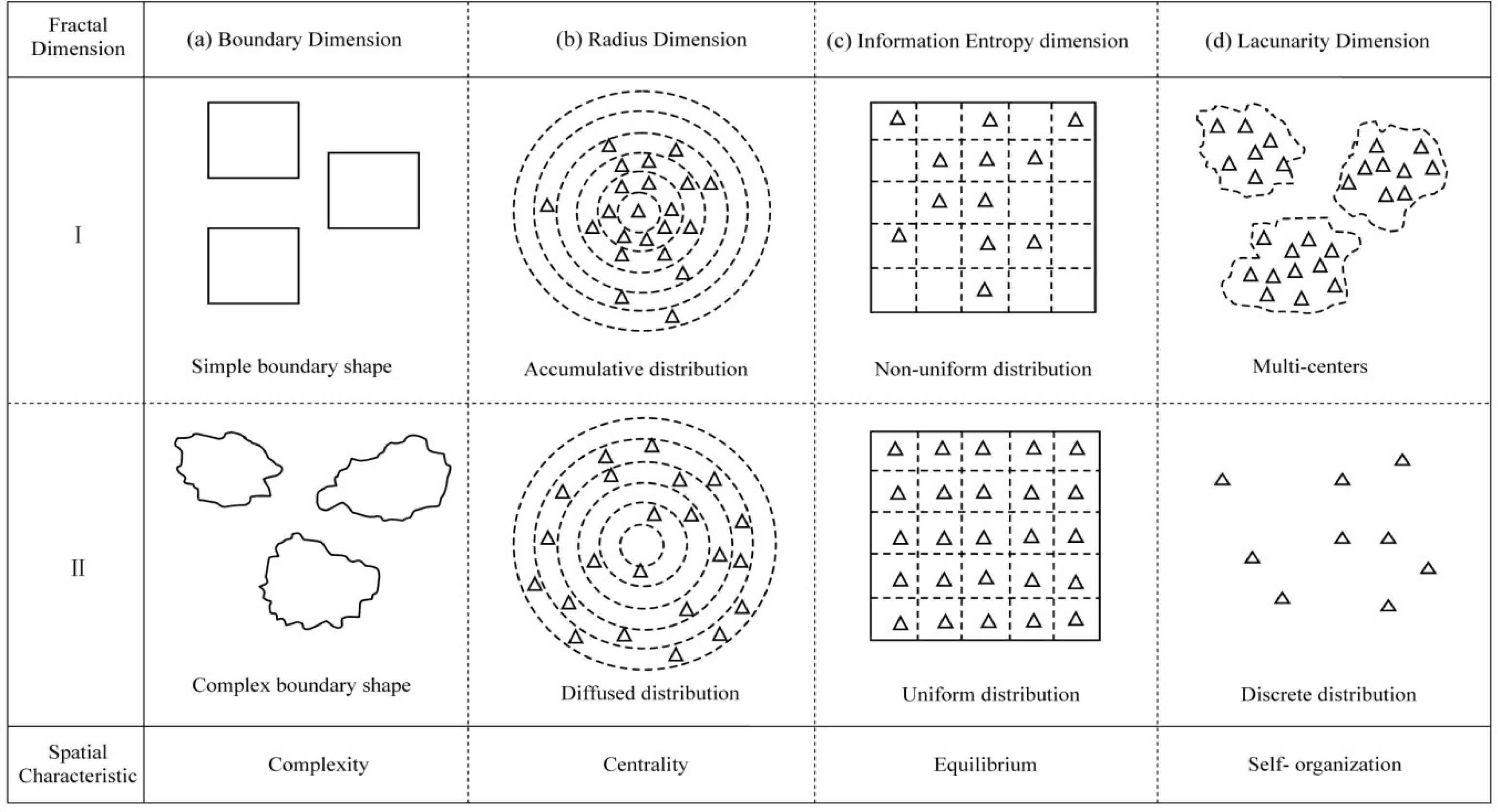
2.1. Three Typical Fractal Dimensions

The boundary dimension calculated using the divider approach [64] was first introduced to measure the city boundary complexity by Longley and Batty [58]. It was gradually applied to the study of land use spatial structure at the micro level. Assuming there was a land patch with an area of A and a perimeter of P, its boundary was characterized by the fractal feature, defined by the fractal dimension D_B. For a certain land use type, the boundary dimension was determined from the area A and the perimeter P for all patches.

$$\text{ln}A=\text{ln}C+2/D_B\times \text{ln}P$$

(1)

where C is a constant coefficient. The boundary dimension D_B, representing the relation between the patch area and the patch perimeter, can measure the complexity and randomicity of land use patches. Its value ranges from 1.0 to 2.0. A value of 1.0 means that the shape of the land use patch is a square, whereas a value of 2.0 represents the most complicated state. When the value is 1.5, it shows a fractal Brownian motion. In other words, the higher the value, the more complex the land boundary becomes.

Another commonly used fractal dimension is the radius dimension proposed by Frankhauser and Sadler [59]. White and Engelen utilized the radius dimension to analyze the spatial patterns of urban land use [60]. The radius dimension was calculated using the mass-radius method [64], which was defined by the total patch area and its radius to depict the density change of a certain land use type radiating outward from a single point at the macro level. It was regarded as an effective evaluation criterion to assess the centrality of urban land use patterns using the relation

$$\text{ln}S(r)=\text{ln}C+D_R\times \text{ln}r$$

(2)

where r is the radius to the urban center; S(r) is the area of a certain land use within the circle with radius r; C is a constant coefficient; and D_R is the radius dimension of a certain land type. When the radius dimension is less than 2.0, the spatial density for a certain land use type decreases nonlinearly outward from the given single point, and the decrease occurs more quickly with a smaller value. Conversely, when the value is greater than 2.0, the spatial density increases outward from the given single point. In particular, the spatial density remains unchanged from the center to external edge when the radius dimension is equal to 2.0. In short, the smaller the value, the stronger the aggregation degree is.

In addition, some researchers have used information entropy to describe the balance for a certain type of urban land use. Although the information entropy index is regarded as a good measure of spatial distribution, it is difficult to compare across different types of land use because of severe spatial scale effects. To solve this problem, Chen and Liu used the box counting method [64] to extend the information entropy to the information entropy dimension by the relation [55]

$$I(\epsilon )=I_0-D_I\times \text{ln}\epsilon$$

(3)

where ε is the grid scale; I₀ is the initial value of information entropy; I(ε) is the information entropy of a certain land use type with the grid scale ε and D_I is the information entropy dimension. The information entropy dimension is designed to explore the overall aggregation degrees of different urban land use types at the macro level. In principle, the value of the information entropy dimension varies from 0 to 2.0. When it is equal to 0, the spatial pattern of land use is concentrated to a point. When it is equal to 2.0, the land presents a uniform spatial distribution. For the remainder of the values, a larger fractal dimension value represents a more even distribution of land use spatial patterns, whereas a smaller value is associated with a more concentrated distribution.

2.2. A Novel Fractal Dimension—Lacunarity Dimension

Although some successful research cases and informative studies on the three fractal dimensions have been performed, as discussed above, the question of how to describe the significant spatial patterns related to many distinct aggregation centers at the macro level remains largely unanswered, and systematic investigations to address such issues are urgently needed.

The novel lacunarity dimension is derived from the landscape spatial index of lacunarity using the box counting method [64] but has a better comparability. In comparison with the existing literature, the focus of our work is to improve lacunarity according to its self-similarity feature at different spatial resolutions [65]. Lacunarity was proposed by Mandelbrot and was then introduced to landscape ecology by Plotnick to describe patterns of spatial dispersion [66–68]. It was regarded as a measure of the gap size of a geometric structure. The gaps or holes in a landscape pattern generate aggregation centers associated with land use distribution. The more gaps or holes, the more aggregation centers. In its calculation process, the pixel value of a known land use type was set to 1 and the pixel value of others to 0. The template, with a size of R×R pixels, was to match the study area pixels from the first row and column and to move one column or row in one step, both from left to right, and from top to bottom. In the matching procedures, the land use type with the value of 1 in the template was counted and recorded as S. After the entire study area was scanned by the template, the occurrence frequency of S was calculated and defined as n(S,R), which was the occurrence frequency of S in all R×R templates. If the study area was composed of M×N pixels and the size of the window template was R×R, the maximum number N(R) of templates R contained in the study area was calculated as follows:

$$N(R)=(M-R+1)\times (N-R+1)$$

(4)

The frequency distribution of n(S,R) was correspondingly transformed to the probability distribution Q(S,R):

$$Q(S,R)=n(S,R)/N(R)$$

(5)

The lacunarity was defined as the ratio of the variance of Q(S,R) to the square of the mean-square deviation of Q(S,R):

$$\mathrm{\Lambda }(R)=Z^{(2)}/{(Z^{(1)})}^2$$

(6)

where Λ(R) is the lacunarity index. The mean-square deviation and the variance can be expressed as follows:

$$Z^{(1)}=\sum _{S=0}^{R^2}\mathit{SQ}(S,R)$$

(7)

$$Z^{(2)}=\sum _{S=0}^{R^2}{S}^{2}Q(S,R)$$

(8)

When the same window template is used to measure the spatial distribution of a certain urban land use type, a lower value of Λ(R) reflects a strong scatter and homogeneity of its spatial distribution, while a higher value of Λ(R) reflects a more significant concentration. However, lacunarity is a scale-dependent measure of heterogeneity or texture [68]. In other words, the value of the lacunarity index is not a constant for a certain study area but depends heavily on the size and density of the sampling grid as well as the topological shape of the land use patch. The lacunarity index maps to a typical modifiable areal unit problem (MAUP), where the values of the lacunarity index will change with different observation scales. Thus, the metrics of lacunarity are not suitable to explain the spatial distribution differences of urban land use at different scales by direct comparison. To solve this problem, a novel fractal dimension is derived from and substituted for the lacunarity index, defined by the logarithmic expression between the lacunarity index and its scale. According to the lacunarity index Λ(R_i) and the grid size R_i(i=2,3, ..., n²), a regression model based on the box counting method was determined from the relation

$$\text{ln}\mathrm{\Lambda }(R_i)={\mathrm{\Lambda }}_0-D_L\times \text{ln}{R}_i$$

(9)

where Λ₀ is the initial value of the lacunarity index and D_L is the lacunarity dimension. A low lacunarity dimension reflects a more scattered spatial distribution of a certain land use type in the study area, while a high lacunarity dimension means a more concentrated spatial distribution. Although we can use the lacunarity dimension to quantify the self-organization features of a certain land use type, it is calculated on the assumption that there exists a fractal feature at different scales. Note that Equation (9) should be subject to the linear regression validation between the lacunarity index and the grid size in the natural logarithm. Figure 2 shows four possible lacunarity index trends with increasing grid size. Figure 2a–c shows three non-linear relationships between the lacunarity index and the grid size in the natural logarithm, while Figure 2d shows an exact linear relationship. Thus, although the lacunarity dimension D_L is defined by Equation (9), it can only work when the lacunarity index and the grid size in natural logarithm are linearly fitted well by the least-squares estimation, as shown in Figure 2d. This fit is both a prerequisite and a limitation for the application of the lacunarity dimension.

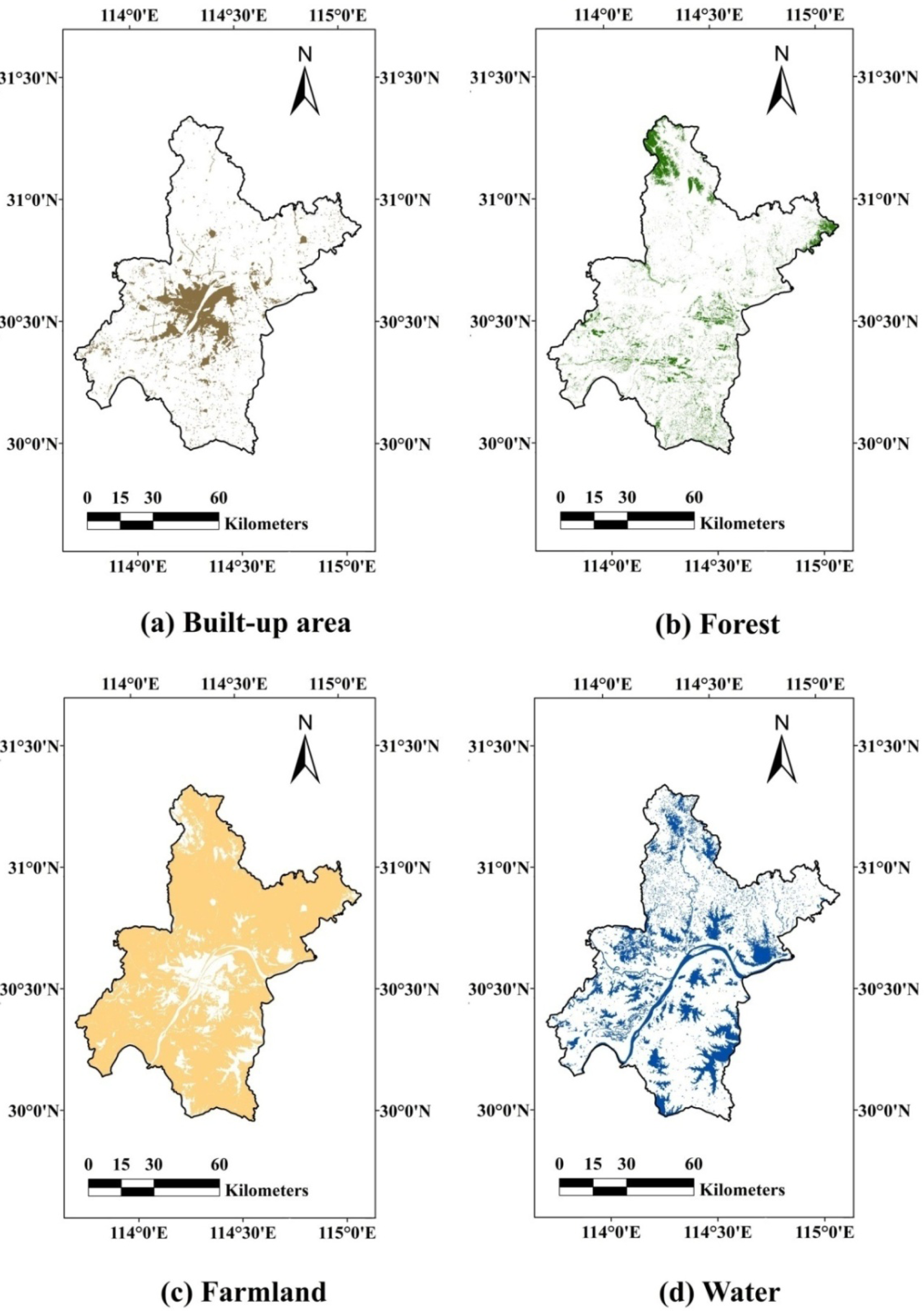
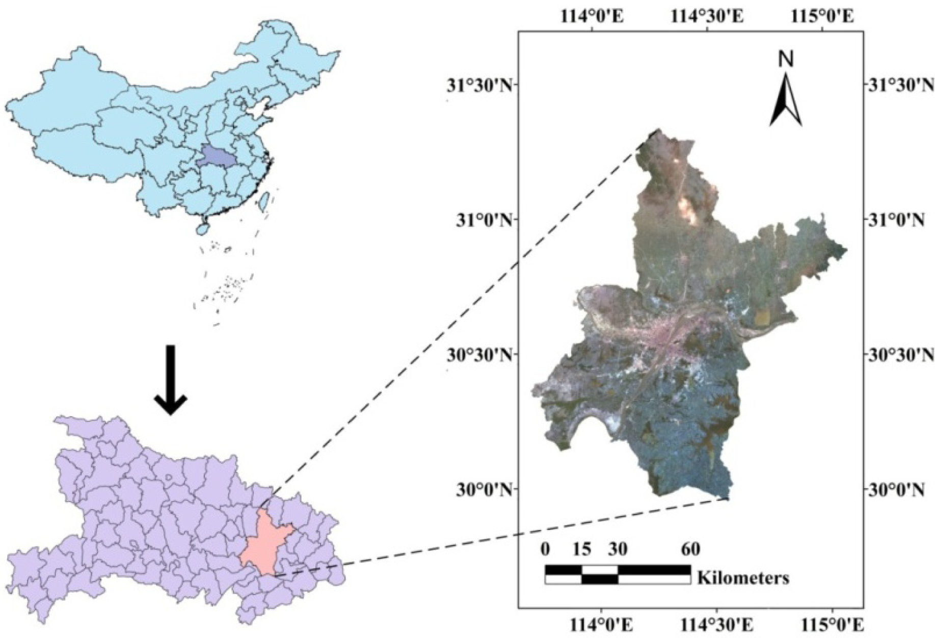
3. Study Area and Data Processing

In this study, Wuhan in central China was selected for study of its urban land use patterns. Wuhan is located in the eastern part of the Jianghan Plain along the middle reach of the Yangtze River, from approximately 113°41′E to 115°05′E, and from 29°58′N to 31°22′N. Wuhan’s climate is humid subtropical with abundant rainfall and four distinct seasons. Its administrative area is almost 8,494 km² with a population of 10,120,000 people. Its major landform is plains, but the area is also covered with hills, lakes, and pools. There are dozens of lakes in this city, which distinguishes it from other metropolises in China; the water areas account for approximately 15% of the entire city, from which the reputation of “the City of a hundred lakes” arises. Red soil and yellow-brown soil are broadly distributed in this area. In the past three decades, this area was profoundly affected by the disturbances of human activity. The Yangtze River and the Hanjiang River meet in Wuhan and divide the central urban area into three parts: Wuchang, Hankou, and Hanyang. As the provincial industrial, educational and administrative center, Wuhan City was taken as the study area, as shown in Figure 3.

A cloud-free Landsat-7 Enhanced Thematic Mapper Plus (ETM+) image (Row/Path: 038/123), collected on 17 September 2010, was acquired from USGS. The image was further rectified to the Universal Transverse Mercator project system (datum WGS84, UTM Zone N49) by a third-order polynomial using the nearest neighbor method, and good geometric correction accuracy was obtained with less than 0.5 pixels. We conducted field investigations to establish a precise classification system. Beforehand, an ISODATA classifier was used to detect subclasses by an unsupervised clustering method in consideration of different reflectance characteristics for different objects within the same land use type. Then, we undertook supervised classification, and the image was classified into six land use classes: unused land, built-up area, water, grassland, forest, and farmland. The data from the filed investigations were used as a reference to evaluate the classification accuracy, and the overall accuracy of the classification result was greater than 90%. The classification result was used to separately extract four raster classification maps to express the spatial patterns of different land use types more clearly. These raster maps were further converted to vector maps, which were then used to identify the spatial features of land use patches by ArcGIS software. The land use patch features were input to calculate the fractal dimensions in Matlab. Due to the small number of patches and areas for grassland and unused land, this study mainly analyzed the other four land use types shown in Figure 4: Built-up area, water, forest and farmland, which accounted for more than 99% of the total number of patches as well as of the total area (

Table 1. The classification results of satellite-detected land use information in Wuhan.

ID	Land Use Types	Number of Patches	Percentage of Patches (%)	Area (m2)	Percentage of Area (%)
1	Built-up area	7,274	10.089	607,801,492	7.075
2	Forest	31,849	44.174	734,558,400	8.550
3	Farmland	15,137	20.995	6,701,792,036	71.023
4	Water	16,864	23.390	1,134,048,588	13.200

).

4. Results and Discussion

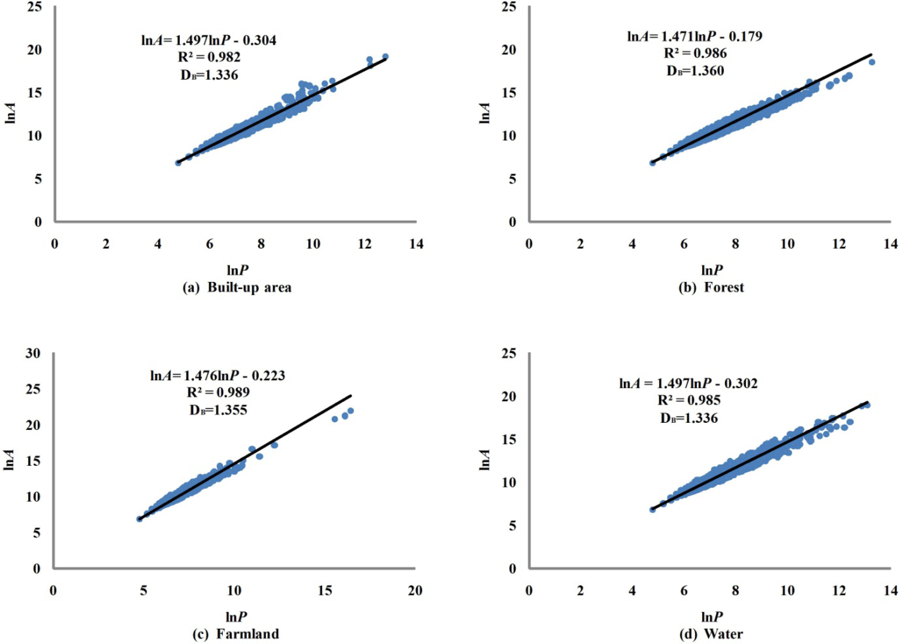
4.1. Boundary Dimension

Statistically significant (p < 0.001) relationships between the logarithm of area and the logarithm of perimeter were established with linear regression analyses. Figure 5 shows that the correlation coefficients (R²) from the least-squares estimation for all four land use types are over 0.980. This result indicates that there are strong linear relationships between lnA and lnP. Thus, it is reasonable to use the boundary dimensions derived from Equation (1) to interpret different land use spatial structures at the micro level.

Figure 5 shows that the four land use types share a common feature of low boundary dimensions, less than 1.5, suggesting that the shape complexities of each single patch are overall relatively simple. However, there are still some remarkable differences among the various land use types. The boundary dimensions of forest and farmland are 1.360 and 1.355, respectively. Both dimensions are close to 1.5, indicating more stochastic boundaries than the water and built-up areas. This result also suggests that the patch boundary shapes of forest and farmland are more irregular and fragmental than the boundary shapes of water and built-up areas. This difference is primarily due to the impacts of destructive agricultural activities and intense human disturbances on the farmland and the forest cover areas, such as regional land consolidation, unsustainable agricultural practices, and uncontrolled deforestation for farming potential. In particular, numerous forests have been converted into farmlands since the family-contract responsibility system, regarded as a significant breakthrough and innovation in the rural land property rights institution of China, was conducted in 1981.

The boundary dimension of the built-up area is relatively low, which manifests as simple boundary shapes related to each single patch as a whole. This phenomenon may be caused by regular outlines derived from remote sensing imagery, which are mostly similar to ordinary geometric shapes, such as rectangles, squares and hexagons. Water, like the built-up area, also has a low boundary dimension value. Being second only to farmland, water accounts for 13.2% of the total area shown in Table 1 and is regarded as playing an important role in the improvement of ecological landscape and the mitigation of the urban heat island. This role has encouraged the government to devote more attention and investment to protecting lakes and rivers in the past ten years than before. For instance, there are many noticeable waterfront sidewalks around East Lake (the largest lake in the central district of China), as well as kilometers of man-made embankments for the cultural landscape on both sides of the Yangtze River. These municipal projects have transformed the random and natural boundaries into regular and artificial ones, creating a low boundary dimension value for water.

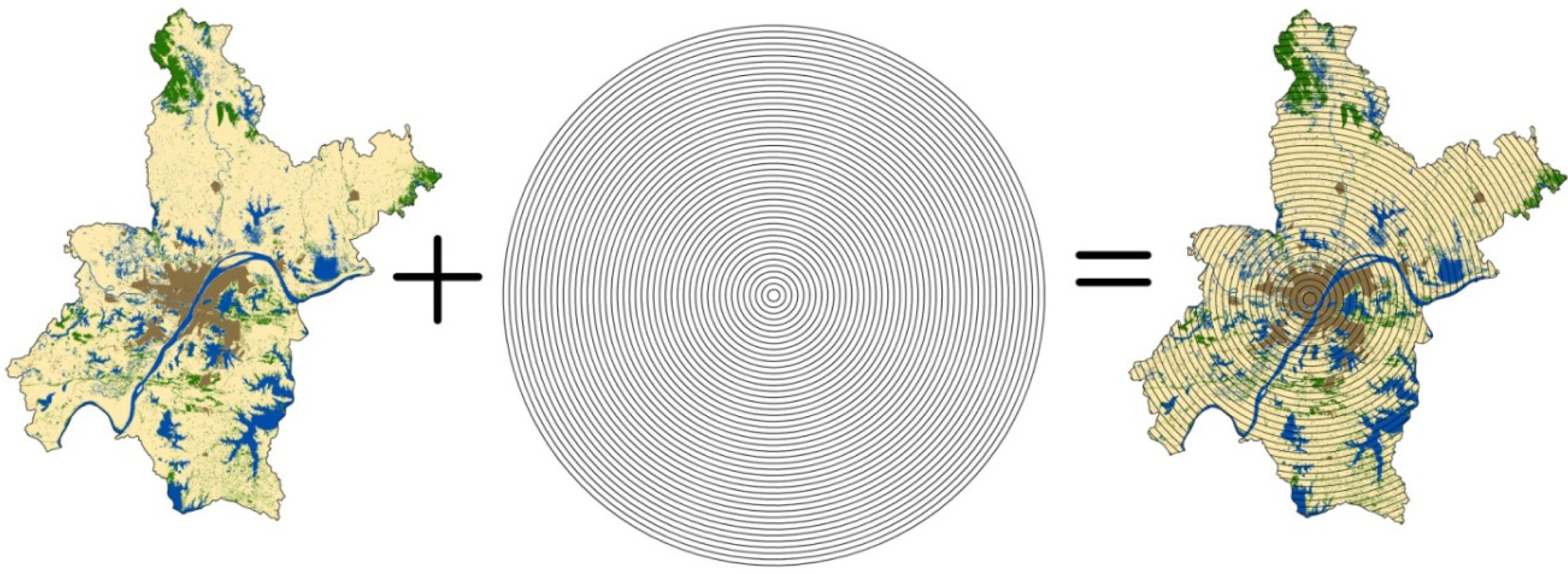
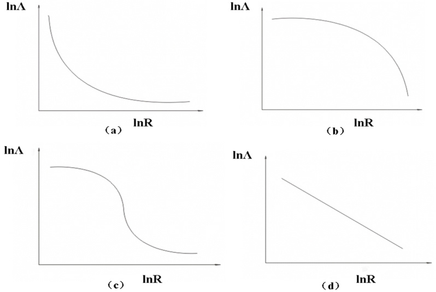
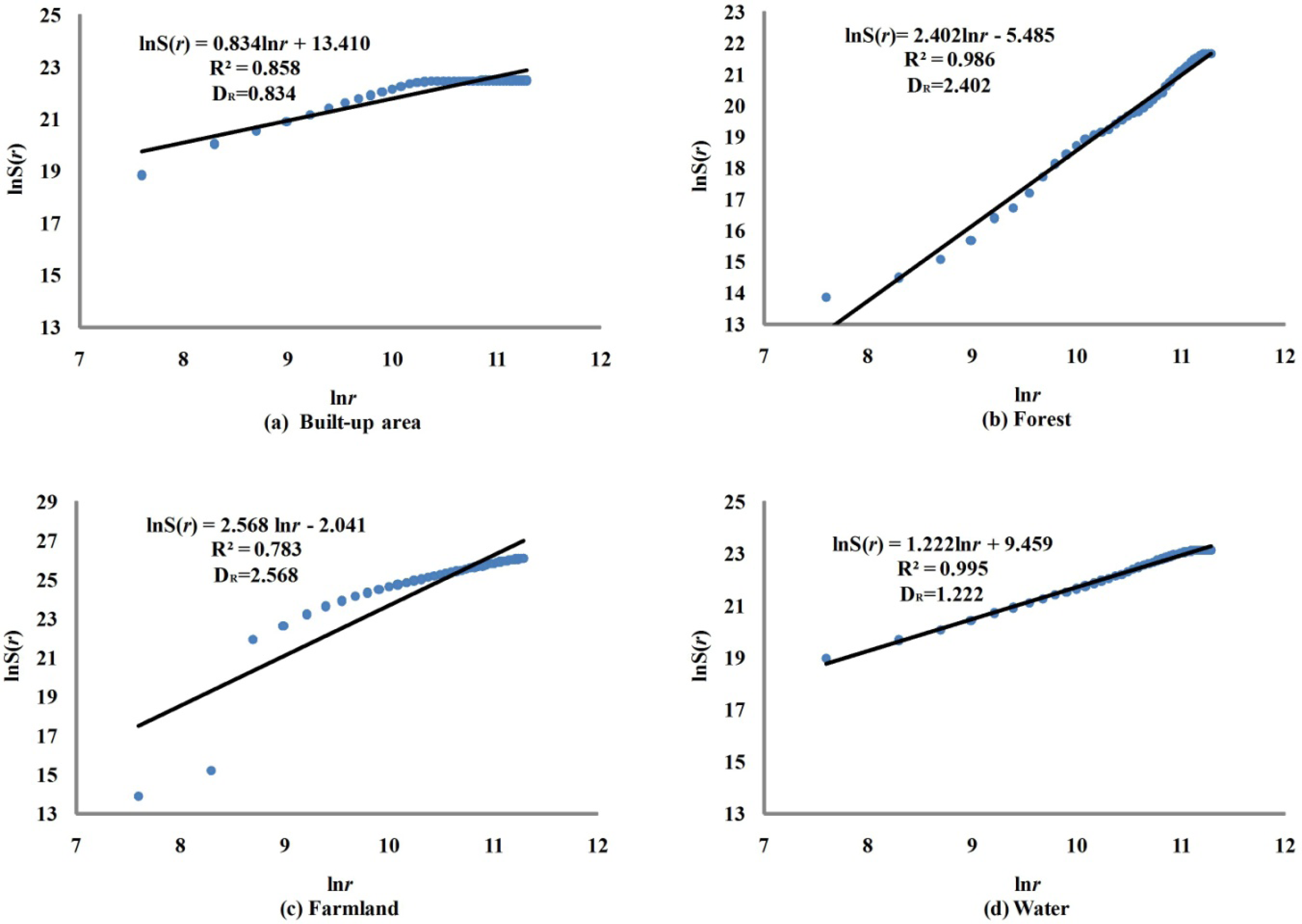
4.2. Radius Dimension

To understand the centrality of land use spatial patterns through the radius dimension, both the location of the analysis center and the interval value of the circle radius shown in Figure 1b need to be studied first. The analysis center generally refers to the urban center, which has three types of basic forms: the geometric outline center, the commercial center and the political hot spot. Because of the urban spatial expansion with economic development in Wuhan, the most famous commercial center is the most suitable measurement center. In this study, the World Trade Plaza Shopping Centre, a landmark building of Wuhan, was chosen as representative of the overall centrality. Another key issue related to the radius dimension is the determination of the radius interval value. Due to the large amount of data involved, it is impractical to perform radius dimension analysis using too small a radius interval for the whole city. In turn, it is also meaningless to adopt a wide interval so that there are too few samples to accurately analyze its tendency based on statistical principles. Therefore, we chose a buffer zone with a width of 2,000 m for the spatial buffer overlay operation (shown in Figure 6) so that there are sufficient samples (more than 40) for regression analysis data but not a heavy computation burden in buffer operation.

Figure 7 shows that there are strong linear relationships between the logarithm of area and the logarithm of radius for all four land use types, which are statistically significant at the 0.001 level. This result suggests that the radius dimension determined by Equation (2) is feasible for quantifying the land use intensity change from the urban center to the outer boundary. Notably, the correlation coefficient of farmland (R² = 0.783) is dramatically lower than the correlation coefficient of the other three types (R² > 0.850), as shown in Figure 7. This difference is caused by an abrupt change of farmland prevalence from the central districts to the rural districts. Figure 4c shows that the change occurs around the boundary of the built-up area, with a few areas of farmland closer to the urban center but a great many far from it. It has been further confirmed by the double logarithmic scatter plot between area and perimeter shown in Figure 7c that there is a distinctive change from the second point to the third one. This situation leads to a relatively poor regression fitting effect for farmland.

A comparison among the four land use types indicates that the farmland yields the highest radius dimension (2.568), followed by the forest (2.402), water (1.222), and built-up area (0.834). This comparison reveals that the farmland is more sharply characterized than the others by an increasing distribution density from urban center to its surrounding area. This tendency of farmland has already been touched upon earlier in the discussion of determining its corresponding correlation coefficient. Although the area of forest is much smaller than the area of farmland, there is a slightly scattered distribution in the northwest, northeast, and southeast regions far from the urban center, as shown in Figure 4b. This distribution results in a radius dimension greater than 2. Both the built-up area and the water have radius dimensions less than 2, which reveals that they have centrality trends, aggregating towards the urban center. However, the radius dimension value of the built-up area is distinctly lower than the radius dimension value of water, indicating a stronger centrality. This result may elucidate the appearance that it is easy to observe the centrality trend for the built-up area in Figure 4a, while the trend for water in Figure 4c is rather blurry.

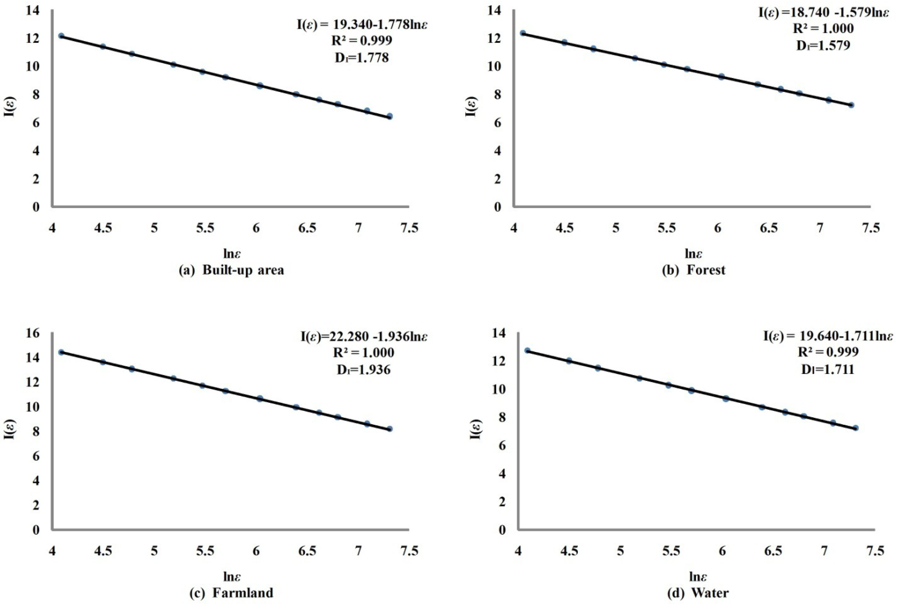
4.3. Information Entropy Dimension

A simple linear regression analysis based on Equation (3) was performed to calculate the information entropy dimension by ordinary least squares. Figure 8 shows that the correlation coefficients for all four land use types exceed 0.999. This result suggests that the fits between I(ε) and lnε are extremely good. The same observation and result associated with the information entropy dimension are fairly well documented in fractal characteristic literature [38]. Therefore, this dimension is reasonable for assessing the balance of land use structure.

The information entropy dimensions of urban land use are ranked in descending order as farmland (1.936), built-up area (1.778), water (1.711), and forest (1.579). This result suggests that the farmland distribution is relatively homogenous compared to the other three land use types. We speculate that this result may reflect its dominance in area over the city. Of those land use types in Wuhan, the farmland area is the largest, accounting for 71.023% of the total area. Although the central districts have a farmland area of less than 10%, as shown in Figure 4c, the suburban and rural districts are dotted with patches of farmland. The information entropy dimension of the forest, on the other hand, is the lowest, indicating a seriously imbalanced spatial distribution. It can be confirmed from Figure 4b that the majority of forest is concentrated in the northeast and northwest, far from urban areas, with small scattered patches in the southeast. This distribution can easily lead to a fragile ecological environment in certain local areas. Thus, efforts should be intensified to develop and conserve forest resources in Wuhan. In addition, the information entropy dimension values of built-up area and water are closer to forest than to farmland, indicating that their land use spatial patterns are not balanced. This result agrees with their spatial distributions shown in Figure 4a and d as well as the results of the radius dimension, as discussed above.

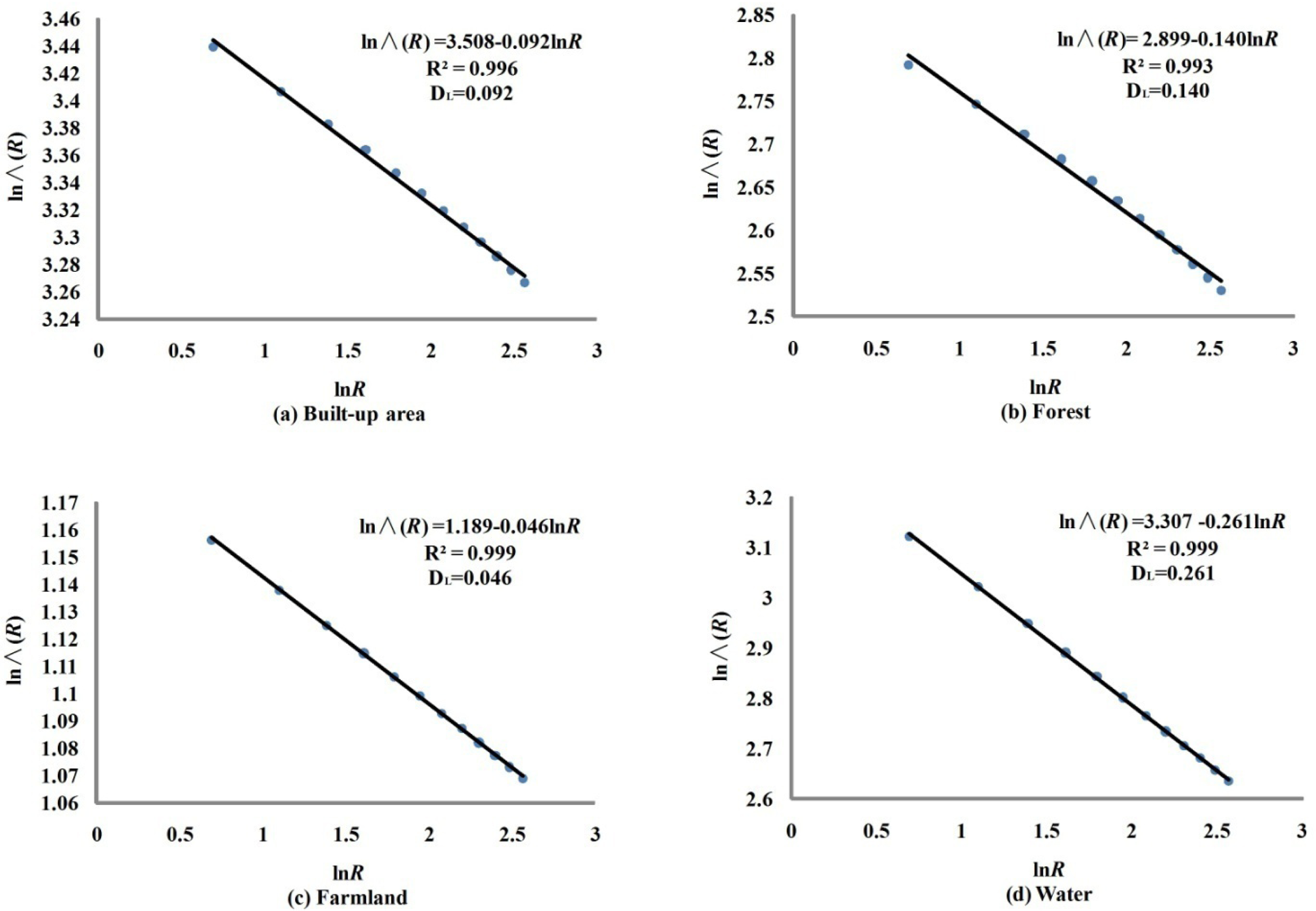
4.4. Lacunarity Dimension

Figure 9 shows that the lacunarity indices of all four land use types decline as the grid size increases. The logarithm of the water lacunarity index, for instance, decreases from 3.14 to 2.62 as the logarithm of the grid size increases from 0.7 to 2.6. That is, the lacunarity index depends heavily on the size of the template. This result reveals that it is meaningless to directly compare the four land use types using the lacunarity index because of the scale effects involved. This problem is the main reason that we use fractal theory to improve the lacunarity index using Equation (9) in this study.

All four land use types have significant linear regression correlations, as shown in Figure 9, which agree with the linear fit tendency presented in Figure 2d. Thus, explaining the degree of concentration of land use using the lacunarity dimension is sound at the macro level. The lacunarity indices of the four land use types can be sorted in descending order as water (0.261), forest (0.140), built-up area (0.092), and farmland (0.046). Both the built-up area and the farmland are smaller than the water and forest, indicating that the former two categories present a more clustered spatial pattern than the latter ones. Combining this information with the status quo of land use shown in Figure 4, we find that large tracts of built-up area are gathered in the central districts, while the farmland aggregates in patches in the rural districts. This result implies that there is no zoning signal for the suburban sprawl with self-organization features in Wuhan. Otherwise, the government will be forced to adopt cluster development to attempt to amend the zoning of land use, which has occurred in most of the municipalities of America. Although the farmland is far away from the city center, it can be considered to aggregate outward around the urban center. To sum up, the spatial self-organization characteristics as measured by the lacunarity dimension show that the built-up area and farmland are both highly distributed around a certain center. However, they present two different self-organization trends with opposite directions: the built-up area gathers towards the urban center, while the farmland diffuses outward from this center. These results in relation to the lacunarity dimension, as shown in Figures 9a,c, are entirely consistent with our earlier radius dimension results in Figures 7a,c, respectively. In this regard, we confirm that there is a specific relationship between the radius dimension and the lacunarity dimension when the spatial pattern of land use has an aggregation tendency with respect to a single given center in the whole urban extent. However, this phenomenon deserves further examination and verification over a larger area in the future.

The land use type of water has the highest lacunarity dimension value, implying a strong distribution characteristic of gathering into pieces. This result is mainly due to an abundance of water areas in Wuhan, as shown in Figure 4d, including the Yangtze River, Han River, Dong Lake, Nan Lake, Sha Lake, Tangxun Lake, and many other lakes and ponds. According to lacunarity dimension theory, there exists a gathering self-organization center for each lake and pond in the land use spatial pattern. This result indicates that the water spatial pattern, with a crowd of scattered individual patches, leads to the maximum lacunarity dimension. The forest, on the other hand, has a lower value than the water, which suggests that the degree of aggregation of forest is weaker than the degree of aggregation of water. This result is also readily intuitive by contrasting Figure 4b,d.

For the land use spatial patterns in Wuhan, the results suggest that the built-up area has relatively simple land use patches. It also presents a rapid downtrend in spatial distribution density from the urban center to the rural area and has an obvious aggregation distribution concentrated around the commercial center. This feature is due to the backward urban planning, maintaining a slow pace of urban-rural integration in Wuhan. Water patches generally have simple spatial boundaries, indicating a strong human influence. The fact that it keeps the second largest total area and is characteristic of their multiple aggregation centers suggests that the local government has paid substantial attention to protecting water resources during the urbanization process. Conversely, the forest is relatively complex in terms of the single patch shape at the micro level but is not obviously aggregative at the macro level. In fact, this is a typical phenomenon of deforestation, which may result from a rapid expansion of the cultivation area on the earth’s surface.

5. Conclusions

A novel approach was proposed to quantify urban land use patterns by using multidimensional fractal indices based on self-similarity and randomness. Three fractal dimensions, including boundary dimension, radius dimension, and the information entropy dimension, were introduced as the typical indices to examine the complexity, centrality, and balance of land use spatial patterns, respectively. A new lacunarity dimension was proposed to describe the self-organization feature with multiple centers of urban land use at the macro level. The main conclusions from this study can be summarized as following:

(1)

The utility of multidimensional fractal indices to analyze the spatial patterns of urban land use proved to be more comprehensive than the utility of any single fractal dimension index. The thorough analysis exhibits accurate spatial pattern detection, including correlation coefficients greater than 0.85 and statistically significant with p < 0.001.

(2)

It is feasible to use the proposed lacunarity dimension to solve the typical modifiable areal unit problem associated with the scale effects of lacunarity index. It can effectively distinguish the self-organization feature (multiple centers) from the centrality (only one center) as well as the balance (no center) of land use spatial patterns at macro level.

(3)

Although the shape complexity of water was found to be highly similar to that of built-up area at micro level in Wuhan, there is a remarkable difference for their macro spatial patterns: Water patches tend to aggregate around multiple individual centers while built-up area only to the urban commercial center.

(4)

It is suggested that we should confirm the goodness of fit and the statistical significance of estimated fractal dimensions before using the multidimensional fractal dimension indices to examine the satellite-detected urban land use spatial patterns.

Despite the achievements in this research, there are several aspects need to be further investigated, such as the effects of classification uncertainties and spatial resolution differences onto fractal analysis. This is beneficial for the government and researchers to gain more accurate insight into the complex spatial patterns of urban land use.

References

1. Carlson, T.N.; Arthur, S.T. The impact of land use-land cover changes due to urbanization on surface microclimate and hydrology: A satellite perspective. Glob. Planet. Chang 2000, 25, 49–65. [Google Scholar]
2. Thapa, R.B.; Murayama, Y. Examining spatiotemporal urbanization patterns in Kathmandu Valley, Nepal: Remote sensing and spatial metrics approaches. Remote Sens 2009, 1, 534–556. [Google Scholar]
3. Vitousek, P.M.; Mooney, H.A.; Lubchenco, J.; Melillo, J.M. Human domination of earth’s ecosystems. Science 1997, 277, 494–499. [Google Scholar]
4. Wu, H.; Zhou, L.; Chi, X.; Li, Y.; Sun, Y. Quantifying and analyzing neighborhood configuration characteristics to cellular automata for land use simulation considering data source error. Earth Sci. Inform 2012, 5, 77–86. [Google Scholar]
5. Dewan, A.M.; Yamaguchi, Y. Land use and land cover change in Greater Dhaka, Bangladesh: Using remote sensing to promote sustainable urbanization. Appl. Geogr 2009, 29, 390–401. [Google Scholar]
6. Dewan, A.M.; Yamaguchi, Y.; Rahman, M.Z. Dynamics of land use/cover changes and the analysis of landscape fragmentation in Dhaka Metropolitan, Bangladesh. GeoJournal 2012, 77, 315–330. [Google Scholar]
7. Herold, M.; Goldstein, N.C.; Clarke, K.C. The spatiotemporal form of urban growth: Measurement, analysis and modeling. Remote Sens. Environ 2003, 86, 286–302. [Google Scholar]
8. Herold, M.; Mayaux, P.; Woodcock, C.E.; Baccini, A.; Schmullius, C. Some challenges in global land cover mapping: An assessment of agreement and accuracy in existing 1 km datasets. Remote Sens. Environ 2008, 112, 2538–2556. [Google Scholar]
9. Xiong, Y.Z.; Huang, S.P.; Chen, F.; Ye, H.; Wang, C.P.; Zhu, C.B. The impacts of rapid urbanization on the thermal environment: A remote sensing study of Guangzhou, South China. Remote Sens 2012, 4, 2033–2056. [Google Scholar]
10. Atzberger, C.; Rembold, F. Mapping the spatial distribution of winter crops at sub-pixel level using AVHRR NDVI time series and neural nets. Remote Sens 2013, 5, 1335–1354. [Google Scholar]
11. Fritz, S.; McCallum, I.; Schill, C.; Perger, C.; Grillmayer, R.; Achard, F.; Kraxner, F.; Obersteiner, M. Geo-Wiki.Org: The use of crowdsourcing to improve global land cover. Remote Sens 2009, 1, 345–354. [Google Scholar]
12. Thenkabail, P.S.; Enclona, E.A.; Ashton, M.S.; Legg, C.; de Dieu, M.J. Hyperion, IKONOS, ALI, and ETM plus sensors in the study of African rainforests. Remote Sens. Environ 2004, 90, 23–43. [Google Scholar]
13. Rudorff, B.F.T.; Aguiar, D.A.; Silva, W.F.; Sugawara, L.M.; Adami, M.; Moreira, M.A. Studies on the rapid expansion of sugarcane for ethanol production in Sao Paulo State (Brazil) using landsat data. Remote Sens 2010, 2, 1057–1076. [Google Scholar]
14. Mundia, C.N.; Aniya, M. Dynamics of land use/cover changes and degradation of Nairobi City, Kenya. Land Degrad. Dev 2006, 17, 97–108. [Google Scholar]
15. Jat, M.K.; Garg, P.K.; Khare, D. Monitoring and modeling of urban sprawl using remote sensing and GIS techniques. Int. J. Appl. Earth Obs. Geoinf 2008, 10, 26–43. [Google Scholar]
16. Dewan, A.M.; Yamaguchi, Y. Using remote sensing and GIS to detect and monitor land use and land cover change in Dhaka Metropolitan of Bangladesh during 1960–2005. Environ. Monit. Assess 2009, 150, 237–249. [Google Scholar]
17. Braimoh, A.K.; Onishi, T. Spatial determinants of urban land use change in Lagos, Nigeria. Land Use Policy 2007, 24, 502–515. [Google Scholar]
18. Foody, G.M. Mapping land cover from remotely sensed data with a softened feedforward neural network classification. J. Intell. Robot. Syst 2000, 29, 433–449. [Google Scholar]
19. Kalluri, S.N.V.; Jaja, J.; Bader, D.A.; Zhang, Z.; Townshend, J.R.G.; Fallah-Adl, H. High performance computing algorithms for land cover dynamics using remote sensing data. Int. J. Remote Sens 2000, 21, 1513–1536. [Google Scholar]
20. Tadesse, W.; Tsegaye, T.; Coleman, T. Land Use/Cover Change Detection of the City of Addis Ababa, Ethiopia Using Remote Sensing and Geographic Information System Technology. Proceedings of IEEE International Geoscience and Remote Sensing Symposium, Sydney, NSW, Australia, 9–13 July 2001.
21. Friedl, M.A.; McIver, D.K.; Hodges, J.C.F.; Zhang, X.Y.; Muchoney, D.; Strahler, A.H.; Woodcock, C.E.; Gopal, S.; Schneider, A.; Cooper, A.; et al. Global land cover mapping from MODIS: Algorithms and early results. Remote Sens. Environ 2002, 83, 287–302. [Google Scholar]
22. Huete, A.R.; Miura, T.; Gao, X. Land cover conversion and degradation analyses through coupled soil-plant biophysical parameters derived from hyperspectral EO-1 Hyperion. IEEE Trans. Geosci. Remote Sens 2003, 41, 1268–1276. [Google Scholar]
23. Gitas, I.Z.; Mitri, G.H.; Ventura, G. Object-based image classification for burned area mapping of Creus Cape, Spain, using NOAA-AVHRR imagery. Remote Sens. Environ 2004, 92, 409–413. [Google Scholar]
24. Thenkabail, P.S.; Schull, M.; Turral, H. Ganges and Indus river basin land use/land cover (LULC) and irrigated area mapping using continuous streams of MODIS data. Remote Sens. Environ 2005, 95, 317–341. [Google Scholar]
25. De Almeida, C.M.; Monteiro, A.M.V.; Soares, G.; Cerqueira, G.C.; Pennachin, C.L.; Batty, M. GIS and remote sensing as tools for the simulation of urban land-use change. Int. J. Remote Sens 2005, 26, 759–774. [Google Scholar]
26. Duran, Z.; Musaoglu, N.; Seker, D.Z. Evaluating urban land use change in historical peninsula, Istanbul, by using gis and remote sensing. Fresenius Environ. Bull 2006, 15, 806–810. [Google Scholar]
27. Chang, L.; Tang, Z.H. Using remote sensing technology to assess land-use changes after the northridge earthquake. Disaster Adv 2010, 3, 5–10. [Google Scholar]
28. Zurita-Milla, R.; Gomez-Chova, L.; Guanter, L.; Clevers, J.G.P.W.; Camps-Valls, G. Multitemporal unmixing of medium-spatial-resolution satellite images: A case study using meris images for land-cover mapping. IEEE Trans. Geosci. Remote Sens 2011, 49, 4308–4317. [Google Scholar]
29. Myint, S.W.; Gober, P.; Brazel, A.; Grossman-Clarke, S.; Weng, Q. Per-pixel vs. object-based classification of urban land cover extraction using high spatial resolution imagery. Remote Sens. Environ 2011, 115, 1145–1161. [Google Scholar]
30. Dymond, J.R.; Shepherd, J.D.; Newsome, P.F.; Gapare, N.; Burgess, D.W.; Watt, P. Remote sensing of land-use change for Kyoto Protocol reporting: The New Zealand case. Environ. Sci. Policy 2012, 16, 1–8. [Google Scholar]
31. Lambin, E.F.; Geist, H.J.; Lepers, E. Dynamics of land-use and land-cover change in tropical regions. Annu. Rev. Environ. Resour 2003, 28, 205–241. [Google Scholar]
32. Le, Q.B.; Park, S.J.; Vlek, P.L.G.; Cremers, A.B. Land-Use Dynamic Simulator (LUDAS): A multi-agent system model for simulating spatio-temporal dynamics of coupled human-landscape system. I. Structure and theoretical specification. Ecol. Inform 2008, 3, 135–153. [Google Scholar]
33. Crews-Meyer, K.A. Agricultural landscape change and stability in northeast Thailand: Historical patch-level analysis. Agric. Ecosyst. Environ 2004, 101, 155–169. [Google Scholar]
34. Wickham, J.D.; Riitters, K.H.; Wade, T.G.; Coulston, J.W. Temporal change in forest fragmentation at multiple scales. Landsc. Ecol 2007, 22, 481–489. [Google Scholar]
35. Roy, P.S.; Tomar, S. Landscape cover dynamics pattern in Meghalaya. Int. J. Remote Sens 2001, 22, 3813–3825. [Google Scholar]
36. Kwan, M.P; Weber, J. Scale and accessibility: Implications for the analysis of land use—Travel interaction. Appl. Geogr 2008, 28, 110–123. [Google Scholar]
37. Schmit, C.; Rounsevell, M.D.A.; La, J.I. The limitations of spatial land use data in environmental analysis. Environ. Sci. Policy 2006, 9, 174–188. [Google Scholar]
38. Ling, Y.Y. The Study of Urban Land Use Structure and Its Non-Linear Transformation (In Chinese). Ms.C. Thesis, East China Normal University, Shanghai, China,. 2004. [Google Scholar]
39. Shi, P.J. Methodology and Practice of Land Use/Cover Change Study; (In Chinese). Science Press: Beijing, China, 2000. [Google Scholar]
40. Weng, Q.H. Fractal analysis of satellite-detected urban heat island effect. Photogramm. Eng. Remote Sens 2003, 69, 555–566. [Google Scholar]
41. De Cola, L. Fractal analysis of a classified Landsat scene. Photogramm. Eng. Remote Sens 1989, 55, 601–610. [Google Scholar]
42. Lam, N.S.N. Description and measurement of landsat TM images using fractals. Photogramm. Eng. Remote Sens 1990, 56, 187–195. [Google Scholar]
43. Lam, N.S.N.; Quattrochi, D.A. On the issues of scale, resolution, and fractal analysis in the mapping sciences. Prof. Geogr 1992, 44, 88–98. [Google Scholar]
44. Myint, S.W.; Lam, N.S.N.; Tyler, J.M. Wavelets for urban spatial feature discrimination: Comparisons with fractal, spatial autocorrelation, and spatial co-occurrence approaches. Photogramm. Eng. Remote Sens 2004, 70, 803–812. [Google Scholar]
45. Emerson, C.W.; Lam, N.S.N.; Quattrochi, D.A. A comparison of local variance, fractal dimension, and Moran’s I as aids to multispectral image classification. Int. J. Remote Sens 2005, 26, 1575–1588. [Google Scholar]
46. Myint, S.W.; Lam, N.S.N. Examining lacunarity approaches in comparison with fractal and spatial autocorrelation techniques for urban mapping. Photogramm. Eng. Remote Sens 2005, 71, 927–937. [Google Scholar]
47. Zhou, G.Y.; Lam, N.S.N. A comparison of fractal dimension estimators based on multiple surface generation algorithms. Comput. Geosci 2005, 31, 1260–1269. [Google Scholar]
48. Myint, S.W.; Mesev, V.; Lam, N.S.N. Urban textural analysis from remote sensor data: Lacunarity measurements based on the differential box counting method. Geogr. Anal 2006, 38, 371–390. [Google Scholar]
49. Ju, W.X.; Lam, N.S.N. An improved algorithm for computing local fractal dimension using the triangular prism method. Comput. Geosci 2009, 35, 1224–1233. [Google Scholar]
50. Zeng, Y.; Zhang, J.; Li, H. Fractal Characteristics of very High Resolution Satellite Imagery. Proceedings of IEEE International Geoscience and Remote Sensing Symposium, Barcelona, Spain, 23–27 July 2007.
51. Emerson, C.W.; Lam, N.S.N.; Quattrochi, D.A. A comparison of local variance, fractal dimension, and Moran’s I as aids to multispectral image classification. Int. J. Remote Sens 2005, 26, 1575–1588. [Google Scholar]
52. Tang, J.; Bu, K.; Yang, J.; Zhang, S.; Chang, L. Multitemporal analysis of forest fragmentation in the upstream region of the Nenjiang River Basin, Northeast China. Ecol. Indic 2012, 23, 597–607. [Google Scholar]
53. Tran, T.D.B.; Puissant, A.; Badariotti, D.; Weber, C. Optimizing spatial resolution of imagery for urban form detection—The cases of France and vietnam. Remote Sens 2011, 3, 2128–2147. [Google Scholar]
54. Liang, B.; Weng, Q.; Tong, X. An evaluation of fractal characteristics of urban landscape in Indianapolis, USA, using multi-sensor satellite images. Int. J. Remote Sens 2013, 34, 804–823. [Google Scholar]
55. Sun, J.; Southworth, J. Remote sensing-based fractal analysis and scale dependence associated with forest fragmentation in an amazon tri-national frontier. Remote Sens 2013, 5, 454–472. [Google Scholar]
56. Sun, W.; Xu, G.; Gong, P.; Liang, S. Fractal analysis of remotely sensed images: A review of methods and applications. Int. J. Remote Sens 2006, 27, 4963–4990. [Google Scholar]
57. Batty, M. Fractals - geometry between dimensions. New Sci 1985, 105, 31–35. [Google Scholar]
58. Batty, M.; Longley, P.A. Fractal-based description of urban form. Environ. Plann. B 1987, 14, 123–134. [Google Scholar]
59. Frankhauser, P.; Sadler, R. Fractal Analysis of Agglomerations. In Natural Structures: Principles, Strategies, and Models in Architecture and Nature; Hilliges, M., Ed.; University of Stuttgart: Stuttgart, Germany, 1991; pp. 57–65. [Google Scholar]
60. White, R.; Engelen, G. Cellular automata and fractal urban form: A cellular modelling approach to the evolution of urban land-use patterns. Environ. Plan. A 1993, 25, 1175–1199. [Google Scholar]
61. Culling, W.E.H. Dimension and entropy in the soil-covered landscape. Earth Surf. Process. Landf 1988, 13, 619–648. [Google Scholar]
62. Martin, M.A.; Rey, J.M.; Taguas, F.J. An entropy-based heterogeneity index for mass-size distributions in Earth science. Ecol. Model 2005, 182, 221–228. [Google Scholar]
63. Wang, D.; Fu, B.; Zhao, W.; Hu, H.; Wang, Y. Multifractal characteristics of soil particle size distribution under different land-use types on the Loess Plateau, China. Catena 2008, 72, 29–36. [Google Scholar]
64. Fernández, E.; Jelinek, H.F. Use of fractal theory in neuroscience: Methods, advantages, and potential problems. Methods 2001, 24, 309–321. [Google Scholar]
65. Dong, P. Lacunarity for spatial heterogeneity measurement in GIS. Geogr. Inf. Sci 2000, 6, 20–26. [Google Scholar]
66. Mandelbrot, B.B. The Fractal Geometry of Nature; W.H. Freeman and Company: New York, NY, USA, 1982. [Google Scholar]
67. Mandelbrot, B.B.; Vespignani, A.; Kaufman, H. Crosscut analysis of large radial DLA: Departures from self-similarity and lacunarity effects. Europhys. Lett 1995, 32, 199–204. [Google Scholar]
68. Plotnick, R.E.; Gardner, R.H.; O’Neill, R.V. Lacunarity indices as measures of landscape texture. Landsc. Ecol 1993, 8, 201–211. [Google Scholar]
Figure 1. Schematic of the Multidimensional Fractal Model (I and II refer to two opposite patch features or spatial distributions for a given land use).
Remotesensing 05 05152f1
Figure 2. Four possible decreasing trends of the lacunarity index: (a) concave curve type, (b) convex curve type, (c) reverse curve type and (d) linear type.
Remotesensing 05 05152f2
Figure 3. Location of Wuhan City.
Remotesensing 05 05152f3
Figure 4. Land use information for four major types in Wuhan: (a) Built-up area, (b) Forest, (c) Farmland and (d) Water.
Remotesensing 05 05152f4
Figure 5. The boundary dimension results for four land use types in Wuhan City: (a) Built-up area, (b) Forest, (c) Farmland and (d) Water.
Remotesensing 05 05152f5
Figure 6. Buffer analysis used to identify area surrounding the given center within different radiuses.
Remotesensing 05 05152f6
Figure 7. The radius dimension results for four land use types in Wuhan City: (a) Built-up area, (b) Forest, (c) Farmland and (d) Water.
Remotesensing 05 05152f7
Figure 8. The information entropy dimension results for four land use types in Wuhan City: (a) Built-up area, (b) Forest, (c) Farmland and (d) Water.
Remotesensing 05 05152f8
Figure 9. The lacunarity dimension results for four land use types in Wuhan City: (a) Built-up area, (b) Forest, (c) Farmland and (d) Water.
Remotesensing 05 05152f9