Allometric Scaling and Resource Limitations Model of Tree Heights: Part 1. Model Optimization and Testing over Continental USA

 ,
, 


Abstract
:
1. Introduction
2. The ASRL Model
3. Data
3.1. Input Data for the ASRL Model
3.1.1. Climate Data
3.1.2. Ancillary Data
3.2. GLAS Tree Heights
4. Methods
4.1. Defining Climatic Zones
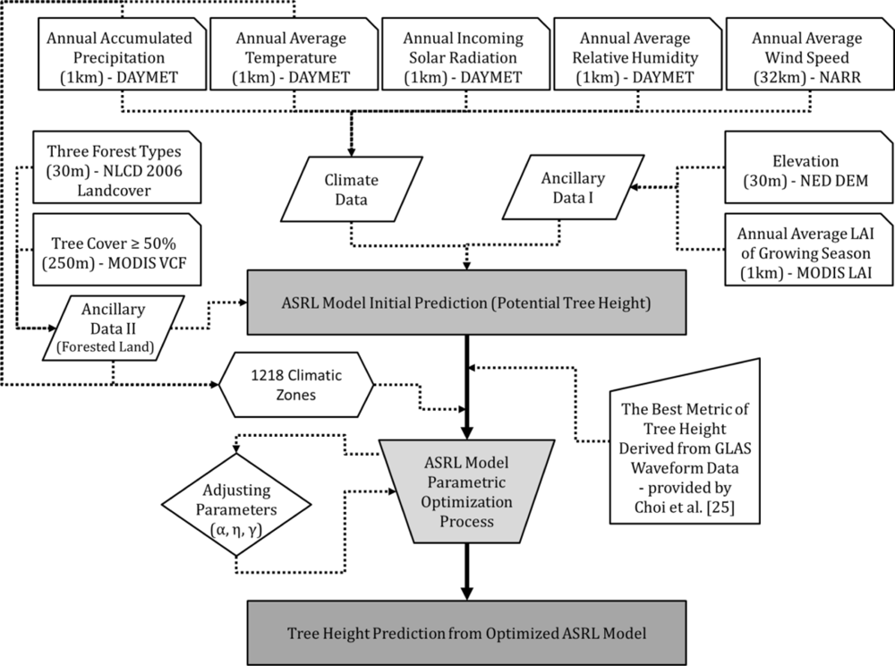
4.2. Initial ASRL Model Prediction of Potential Tree Heights
4.3. Optimization of the ASRL Model
4.4. Evaluation of the Optimized ASRL Model Results
4.4.1. Two-Fold Cross Validation
4.4.2. Inter-comparison with Other Forest Height Maps
5. Results and Discussion
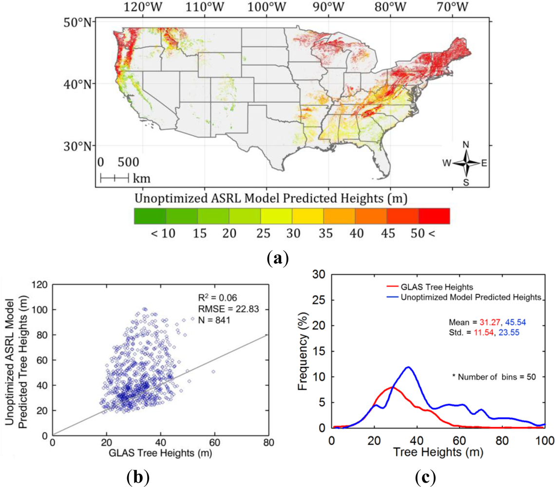
5.1. Initial ASRL Model Predictions of Potential Tree Heights
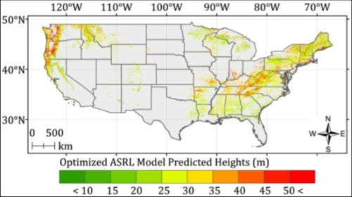
5.2. Optimized ASRL Model Predictions
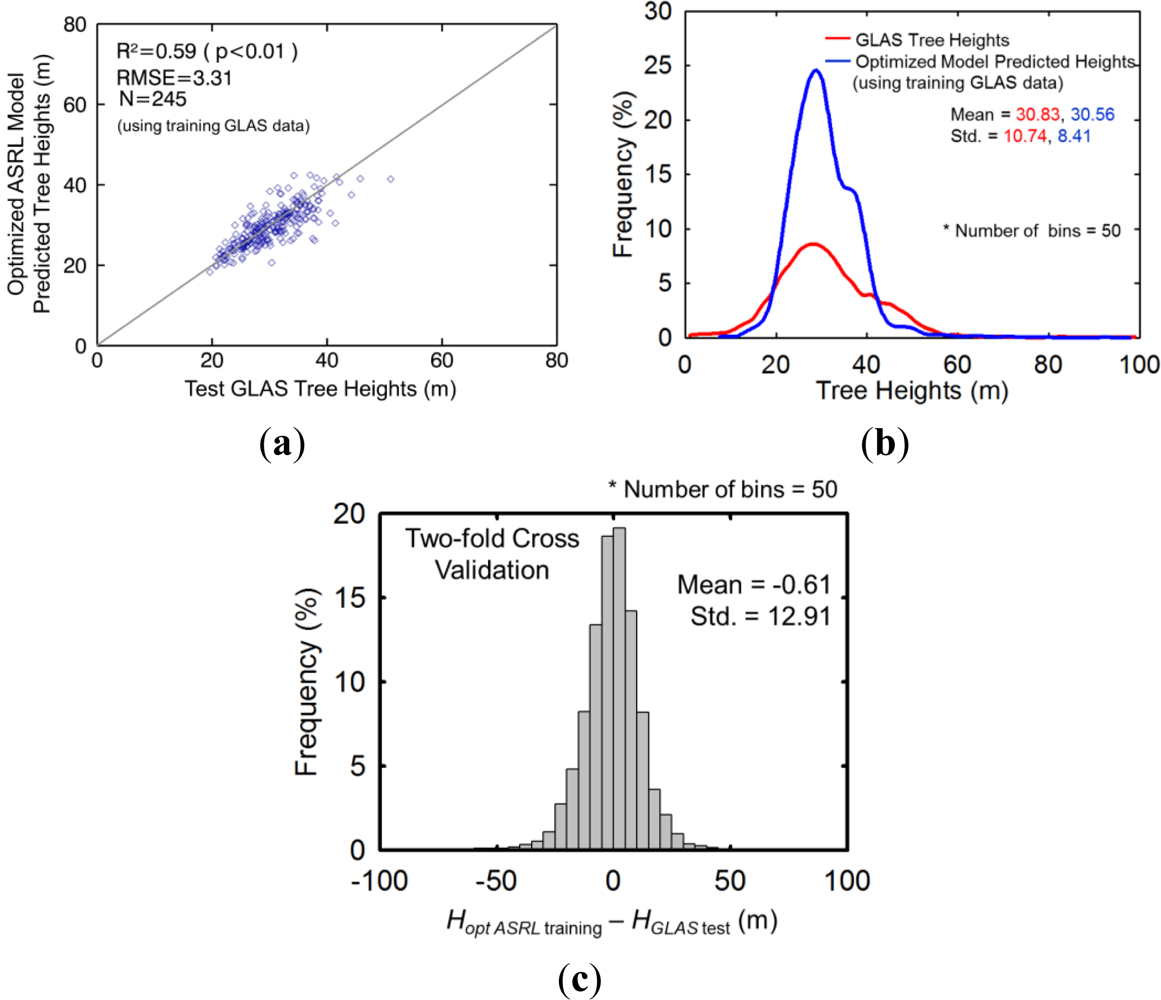
5.3. Evaluation of the Optimized ASRL Model
5.3.1. Two-Fold Cross Validation Approach
5.3.2. Inter-comparison with Other Forest Height Maps
6. Concluding Remarks
Supplementary Information
remotesensing-05-00284-s001.docxAcknowledgments
References
- Simard, M.; Pinto, N.; Fisher, J.B.; Baccini, A. Mapping forest canopy height globally with spaceborne lidar. J. Geophys. Res.-Biogeosci. 2011, 116. [Google Scholar] [CrossRef]
- Lefsky, M.A. A global forest canopy height map from the Moderate Resolution Imaging Spectroradiometer and the Geoscience Laser Altimeter System. Geophys. Res. Lett. 2010, 37. [Google Scholar] [CrossRef]
- Zhang, G.; Ganguly, S.; Nemani, R.; White, M.; Milesi, C.; Wang, W.; Saatchi, S.; Yu, Y.; Myneni, R.B. A simple parametric estimation of live forest aboveground biomass in California using satellite derived metrics of canopy height and Leaf Area Index. Geophys. Res. Lett. 2012. under review.. [Google Scholar]
- Saatchi, S.S.; Harris, N.L.; Brown, S.; Lefsky, M.; Mitchard, E.T.A.; Salas, W.; Zutta, B.R.; Buermann, W.; Lewis, S.L.; Hagen, S.; Petrova, S.; White, L.; Silman, M.; Morel, A. Benchmark map of forest carbon stocks in tropical regions across three continents. Proc. Natl. Acad. Sci. USA 2011, 108, 9899–9904. [Google Scholar]
- Chopping, M.; Schaaf, C.B.; Zhao, F.; Wang, Z.S.; Nolin, A.W.; Moisen, G.G.; Martonchik, J.V.; Bull, M. Forest structure and aboveground biomass in the southwestern United States from MODIS and MISR. Remote Sens. Environ 2011, 115, 2943–2953. [Google Scholar]
- Sun, G.; Ranson, K.J.; Kimes, D.S.; Blair, J.B.; Kovacs, K. Forest vertical structure from GLAS: An evaluation using LVIS and SRTM data. Remote Sens. Environ 2008, 112, 107–117. [Google Scholar]
- Mitchard, E.T.A.; Saatchi, S.S.; Lewis, S.L.; Feldpausch, T.R.; Gerard, F.F.; Woodhouse, I.H.; Meir, P. Comment on “A first map of tropical Africa’s above-ground biomass derived from satellite imagery”. Environ. Res. Lett. 2011, 6. [Google Scholar] [CrossRef]
- Selkowitz, D.J.; Green, G.; Peterson, B.; Wylie, B. A multi-sensor lidar, multi-spectral and multi-angular approach for mapping canopy height in boreal forest regions. Remote Sens. Environ 2012, 121, 458–471. [Google Scholar]
- Jung, S.-E.; Kwak, D.-A.; Park, T.; Lee, W.-K.; Yoo, S. Estimating crown variables of individual trees using airborne and terrestrial laser scanners. Remote Sens 2011, 3, 2346–2363. [Google Scholar]
- Straub, C.; Koch, B. Estimating single tree stem volume of Pinus sylvestris using airborne laser scanner and multispectral line scanner data. Remote Sens 2011, 3, 929–944. [Google Scholar]
- Treuhaft, R.N.; Chapman, B.D.; dos Santos, J.R.; Goncalves, F.G.; Dutra, L.V.; Graca, P.M.L.A.; Drake, J.B. Vegetation profiles in tropical forests from multibaseline interferometric synthetic aperture radar, field, and lidar measurements. J. Geophys. Res.-Atmos. 2009, 114. [Google Scholar] [CrossRef]
- Treuhaft, R.N.; Goncalves, F.G.; Drake, J.B.; Chapman, B.D.; dos Santos, J.R.; Dutra, L.V.; Graca, P.M.L.A.; Purcell, G.H. Biomass estimation in a tropical wet forest using Fourier transforms of profiles from lidar or interferometric SAR. Geophys. Res. Lett. 2010, 37. [Google Scholar] [CrossRef]
- Baccini, A.; Goetz, S.J.; Walker, W.S.; Laporte, N.T.; Sun, M.; Sulla-Menashe, D.; Hackler, J.; Beck, P.S.A.; Dubayah, R.; Friedl, M.A.; Samanta, S.; Houghton, R.A. Estimated carbon dioxide emissions from tropical deforestation improved by carbon-density maps. Nature Clim. Change 2012, 2, 182–185. [Google Scholar]
- Kempes, C.P.; West, G.B.; Crowell, K.; Girvan, M. Predicting maximum tree heights and other traits from allometric scaling and resource limitations. Plos One 2011, 6. [Google Scholar] [CrossRef] [Green Version]
- Kozlowski, J.; Konarzewski, M. Is West, Brown and Enquist’s model of allometric scaling mathematically correct and biologically relevant? Funct. Ecol 2004, 18, 283–289. [Google Scholar]
- Kozlowski, J.; Konarzewski, M. West, Brown and Enquist’s model of allometric scaling again: The same questions remain. Funct. Ecol 2005, 19, 739–743. [Google Scholar]
- Zianis, D. Predicting mean aboveground forest biomass and its associated variance. Forest Ecol. Manage 2008, 256, 1400–1407. [Google Scholar]
- Etienne, R.S.; Apol, M.E.F.; Olff, H. Demystifying the West, Brown & Enquist model of the allometry of metabolism. Funct. Ecol 2006, 20, 394–399. [Google Scholar]
- Brown, J.H.; Gillooly, J.F.; Allen, A.P.; Savage, V.M.; West, G.B. Response to forum commentary on “toward a metabolic theory of ecology”. Ecology 2004, 85, 1818–1821. [Google Scholar]
- Brown, J.H.; West, G.B.; Enquist, B.J. Yes, West, Brown and Enquist’s model of allometric scaling is both mathematically correct and biologically relevant. Funct. Ecol 2005, 19, 735–738. [Google Scholar]
- Enquist, B.J.; West, G.B.; Brown, J.H. Extensions and evaluations of a general quantitative theory of forest structure and dynamics. Proc. Natl. Acad. Sci. USA 2009, 106, 7046–7051. [Google Scholar]
- West, G.B.; Enquist, B.J.; Brown, J.H. A general quantitative theory of forest structure and dynamics. Proc. Natl. Acad. Sci. USA 2009, 106, 7040–7045. [Google Scholar]
- Chojnacky, D.C. Allometric Scaling Theory Applied to FIA Biomass Estimation. In Proceedings of the Third Annual Forest Inventory and Analysis Symposium; McRoberts, R.E., Reams, G.A., Van Deusen, P.C., Moser, J.W., Eds.; Gen. Tech. Rep. NC-230; North Central Research Station, USDA, Forest Service: St. Paul, MN, USA, 2002; Volume 230, pp. 96–102. [Google Scholar]
- Cheng, D.L.; Li, T.; Zhong, Q.L.; Wang, G.X. Scaling relationship between tree respiration rates and biomass. Biol. Lett 2010, 6, 715–717. [Google Scholar]
- Choi, S.; Ni, S.; Shi, Y.; Ganguly, S.; Zhang, G.; Duong, H.V.; Lefsky, M.A.; Simard, M.; Saatchi, S.S.; Lee, S.; et al. Allometric scaling and resource limitations model of tree heights: Part 2. Site based testing of the model. Remote Sens 2013, 5, 202–223. [Google Scholar]
- ESRI. ArcGIS Desktop 9.2 Help Desk: Resampling Under Data Management. Available online: http://webhelp.esri.com/arcgisdesktop/9.2/index.cfm?TopicName=resample_(data_management) (accessed on 12 July 2012).
- Luo, W.; Taylor, M.C.; Parker, S.R. A comparison of spatial interpolation methods to estimate continuous wind speed surfaces using irregularly distributed data from England and Wales. Int. J. Climatol 2008, 28, 947–959. [Google Scholar]
- DAYMET. Available online: http://www.daymet.org/ (accessed on 12 July 2012).
- World Meteorological Organization (WMO). Guide to Meteorological Instruments and Methods of Observation, Appendix 4B; WMO-No. 8 (CIMO Guide); WMO: Geneva, Switzerland, 2008. [Google Scholar]
- North American Regional Reanalysis (NARR). Available online: http://www.emc.ncep.noaa.gov/mmb/rreanl/ (accessed on 12 July 2012).
- Gesch, D.; Evans, G.; Mauck, J.; Hutchinson, J.; Carswell, W.J. The National Map—Elevation: U.S. Geological Survey Fact Sheet 2009-3053, 2009; 4.
- Yuan, H.; Dai, Y.J.; Xiao, Z.Q.; Ji, D.Y.; Wei, S.G. Reprocessing the MODIS Leaf Area Index products for land surface and climate modelling. Remote Sens. Environ 2011, 115, 1171–1187. [Google Scholar]
- Fry, J.A.; Xian, G.; Jin, S.M.; Dewitz, J.A.; Homer, C.G.; Yang, L.M.; Barnes, C.A.; Herold, N.D.; Wickham, J.D. Completion of the 2006 National Land Cover Database for the Conterminous United States. Photogramm. Eng. Remote Sensing 2011, 77, 859–864. [Google Scholar]
- Hansen, M.C.; DeFries, R.S.; Townshend, J.R.G.; Carroll, M.; Dimiceli, C.; Sohlberg, R.A. Global percent tree cover at a spatial resolution of 500 meters: First results of the MODIS Vegetation Continuous Fields Algorithm. Earth Interact 2003, 7, 1–10. [Google Scholar]
- Zwally, H.J.; Schutz, B.; Abdalati, W.; Abshire, J.; Bentley, C.; Brenner, A.; Bufton, J.; Dezio, J.; Hancock, D.; Harding, D.; et al. ICESat’s laser measurements of polar ice, atmosphere, ocean, and land. J. Geodyn 2002, 34, 405–445. [Google Scholar]
- Abshire, J.B.; Sun, X.L.; Riris, H.; Sirota, J.M.; McGarry, J.F.; Palm, S.; Yi, D.H.; Liiva, P. Geoscience Laser Altimeter System (GLAS) on the ICESat mission: On-orbit measurement performance. Geophys. Res. Lett. 2005, 32. [Google Scholar] [CrossRef]
- Brenner, A.C.; Bentley, C.R.; Csatho, B.M.; Harding, D.J.; Hofton, M.A.; Minster, J.; Roberts, L.; Saba, J.L.; Schutz, R.; Thomas, R.H.; Yi, D.; Zwally, H.J. Derivation of Range and Range Distributions from Laser Pulse Waveform Analysis for Surface Elevations, Roughness, Slope, and Vegetation Heights; Algorithm Theoretical Basis Document Version 4.1; NASA Goddard Space Flight Center: Greenbelt, MD, USA, 2003; p. 12. [Google Scholar]
- Neuenschwander, A.L.; Urban, T.J.; Gutierrez, R.; Schutz, B.E. Characterization of ICESat/GLAS waveforms over terrestrial ecosystems: Implications for vegetation mapping. J. Geophys. Res.-Biogeosci 2008, 113. [Google Scholar] [CrossRef]
- Gong, P.; Li, Z.; Huang, H.B.; Sun, G.Q.; Wang, L. ICESat GLAS data for urban environment monitoring. IEEE Trans. Geosci. Remote Sens 2011, 49, 1158–1172. [Google Scholar]
- Lee, S.; Ni-Meister, W.; Yang, W.Z.; Chen, Q. Physically based vertical vegetation structure retrieval from ICESat data: Validation using LVIS in White Mountain National Forest, New Hampshire, USA. Remote Sens. Environ 2011, 115, 2776–2785. [Google Scholar]
- Chen, Q. Retrieving vegetation height of forests and woodlands over mountainous areas in the Pacific Coast region using satellite laser altimetry. Remote Sens. Environ 2010, 114, 1610–1627. [Google Scholar]
- Lefsky, M.A.; Keller, M.; Pang, Y.; de Camargo, P.B.; Hunter, M.O. Revised method for forest canopy height estimation from Geoscience Laser Altimeter System waveforms. J. Appl. Remote Sens 2007, 1. [Google Scholar] [CrossRef]
- Duncanson, L.I.; Niemann, K.O.; Wulder, M.A. Estimating forest canopy height and terrain relief from GLAS waveform metrics. Remote Sens. Environ 2010, 114, 138–154. [Google Scholar]
- Pang, Y.; Lefsky, M.; Sun, G.Q.; Ranson, J. Impact of footprint diameter and off-nadir pointing on the precision of canopy height estimates from spaceborne lidar. Remote Sens. Environ 2011, 115, 2798–2809. [Google Scholar]
- Harding, D.J.; Carabajal, C.C. ICESat waveform measurements of within-footprint topographic relief and vegetation vertical structure. Geophys. Res. Lett. 2005, 32. [Google Scholar] [CrossRef]
- Neuenschwander, A.L. Evaluation of waveform deconvolution and decomposition retrieval algorithms for ICESat/GLAS data. Can. J. Remote Sens 2008, 34, S240–S246. [Google Scholar]
- Rosette, J.A.B.; North, P.R.J.; Suarez, J.C.; Los, S.O. Uncertainty within satellite LiDAR estimations of vegetation and topography. Int. J. Remote Sens 2010, 31, 1325–1342. [Google Scholar]
- Lagerloef, G.S.E.; Bernstein, R.L. Empirical orthogonal function-analysis of Advanced Very High-Resolution Radiometer surface-temperature patterns in Santa-Barbara Channel. J. Geophys. Res.-Oceans 1988, 93, 6863–6873. [Google Scholar]
- Choi, S.; Lee, W.K.; Son, Y.; Yoo, S.; Lim, J.H. Changes in the distribution of South Korean forest vegetation simulated using thermal gradient indices. Sci. China Life Sci 2010, 53, 784–797. [Google Scholar]
- Powell, M.J.D. An efficient method for finding the minimum of a function of several variables without calculating derivatives. Comput. J 1964, 7, 155–162. [Google Scholar]
- Press, W.H.; Teukolsky, S.A.; Vetterling, W.T.; Flannery, B.P. Minimization or Maximization of Functions. In Numerical Recipes in FORTRAN: The Art of Scientific Computing, 2nd ed.; Chapter 10; Cambridge University Press: Cambridge, UK/New York, NY, USA, 1992; pp. 394–445. [Google Scholar]
- Kuusk, A.; Nilson, T. A directional multispectral forest reflectance model. Remote Sens. Environ 2000, 72, 244–252. [Google Scholar]
- TRY. Plant Trait Database. Available online: http://www.try-db.org/TryWeb/Home.php (accessed on 12 July 2012).
- Kattge, J.; Diaz, S.; Lavorel, S.; Prentice, C.; Leadley, P.; Bonisch, G.; Garnier, E.; Westoby, M.; Reich, P.B.; Wright, I.J.; et al. TRY—A global database of plant traits. Glob. Change Biol 2011, 17, 2905–2935. [Google Scholar]
- West, G.B.; Brown, J.H.; Enquist, B.J. A general model for the structure and allometry of plant vascular systems. Nature 1999, 400, 664–667. [Google Scholar]
- Ridler, M.E.; Sandholt, I.; Butts, M.; Lerer, S.; Mougin, E.; Timouk, F.; Kergoat, L.; Madsen, H. Calibrating a soil–vegetation–atmosphere transfer model with remote sensing estimates of surface temperature and soil surface moisture in a semi arid environment. J. Hydrol. 2012, 436–437, 1–12. [Google Scholar]
- Gholz, H.L. Environmental limits on aboveground net primary production, leaf area, and biomass in vegetation zones of the Pacific Northwest. Ecology 1982, 63, 469–481. [Google Scholar]
- Smith, T.M.; Shugart, H.H.; Bonan, G.B.; Smith, J.B. Modeling the potential response of vegetation to global climate change. Adv. Ecol. Res 1992, 22, 93–116. [Google Scholar]
- Obrien, S.T.; Hubbell, S.P.; Spiro, P.; Condit, R.; Foster, R.B. Diameter, height, crown, and age relationships in 8 neotropical tree species. Ecology 1995, 76, 1926–1939. [Google Scholar]
- Shugart, H.H.; Saatchi, S.; Hall, F.G. Importance of structure and its measurement in quantifying function of forest ecosystems. J. Geophys. Res-Biogeo. 2010, 115. [Google Scholar] [CrossRef]
- Ryan, M.G.; Yoder, B.J. Hydraulic limits to tree height and tree growth. Bioscience 1997, 47, 235–242. [Google Scholar]
- Pan, Y.; Chen, J.M.; Birdsey, R.; McCullough, K.; He, L.; Deng, F. Age structure and disturbance legacy of North American forests. Biogeosciences 2011, 8, 715–732. [Google Scholar]
- Nadeau, C.; Bengio, Y. Inference for the generalization error. Mach. Learn 2003, 52, 239–281. [Google Scholar]
- Wu, J.; Jelinski, D.E.; Luck, M.; Tueller, P.T. Multiscale Analysis of Landscape Heterogeneity: Scale Variance and Pattern Metrics. Geogr. Inf. Sci 2000, 6, 6–19. [Google Scholar]
- Wu, H.; Li, Z.L. Scale issues in remote sensing: A review on analysis, processing and modeling. Sensors 2009, 9, 1768–1793. [Google Scholar]
- Seong, J.C. Modelling the accuracy of image data reprojection. Int. J. Remote Sens 2003, 24, 2309–2321. [Google Scholar]
- Pandey, G.R.; Cayan, D.R.; Dettinger, M.D.; Georgakakos, K.P. A hybrid orographic plus statistical model for downscaling daily precipitation in northern California. J. Hydrometeorol 2000, 1, 491–506. [Google Scholar]
- Lundquist, J.D.; Cayan, D.R. Surface temperature patterns in complex terrain: Daily variations and long-term change in the central Sierra Nevada, California. J. Geophys. Res.-Atmos. 2007, 112. [Google Scholar] [CrossRef]
- Parkhurst, D.F.; Loucks, O.L. Optimal leaf size in relation to environment. J. Ecol 1972, 60, 505–537. [Google Scholar]
- Grier, C.C.; Running, S.W. Leaf area of mature Northwestern Coniferous Forests—Relation to site water-balance. Ecology 1977, 58, 893–899. [Google Scholar]
- Westoby, M.; Falster, D.S.; Moles, A.T.; Vesk, P.A.; Wright, I.J. Plant ecological strategies: Some leading dimensions of variation between species. Annu. Rev. Ecol. Syst 2002, 33, 125–159. [Google Scholar]
- Golluscio, R.A.; Oesterheld, M. Water use efficiency of twenty-five co-existing Patagonian species growing under different soil water availability. Oecologia 2007, 154, 207–217. [Google Scholar]
- Goldstein, G.; Rada, F.; Rundel, P.; Azocar, A.; Orozco, A. Gas-exchange and water relations of evergreen and deciduous tropical savanna trees. Ann. Sci. Forest 1989, 46, S448–S453. [Google Scholar]
- Medina, E.; Francisco, M. Photosynthesis and water relations of savanna tree species differing in leaf phenology. Tree Physiol 1994, 14, 1367–1381. [Google Scholar]


| Categories | Variables | Symbols | Key Equations | Sub-Variables |
|---|---|---|---|---|
| Equations of Basal Metabolic Rates | Available Flow Rate | Qp | Qp = γ π rroot2Pinc | γ = Root Absorption Efficiency; rroot = Radial Extent of Root System; Pinc = Incoming Precipitation Rate |
| Evaporative Flow Rate | Qe | Qe = af Ecan μw ρw−1 | af = Effective Area over the Latent Heat Flux Loss; Ecan = Evaporative Flux of Canopy; μw = Molar Mass of Water (= 1.80 × 10⁻² kg·mol−1); ρw = Density of Water (= 1.0 × 10³ kg·m−3) | |
| Required Flow Rate | Q0 | Q0 = β2hη2 | β2 = Proportionality Constant for Metabolism (≈9.2 × 10⁻⁷ L·day−1 cm·−η2); h = tree height; η2 = Exponent for Metabolism (≈2.7) | |
| Sub-equations of Evaporative Flow Rate | Effective Area over the Latent Heat Flux Loss | af | af = 2 aL δs as | aL = Total One-sided Area of All Leaves on a Tree; δs = Density of Stomata on a Leaf (=220 stomata mm−2); as = Area of a Single Stomata (=235.1 μm2) |
| Total One-sided Area of All Leaves on a Tree | aL | aL = α nN | α = Area of Single Leaf; n = Branching Parameter (=2); N = Number of Branching Generations | |
| Number of Branching Generations | N | N = 2 ln (r0/rN)/ln n | r0 = Maximum Stem Radius; rN = Radius of Terminal Branch (=0.4 mm) | |
| Evaporative Flux of Canopy | Ecan | Refers to [14] | Equation uses Rate of Absorbed Solar Radiation (Rabs) along with Canopy Radius (rcan) and Area of Single Leaf (α) | |
| Sub-allometric Scaling Equations | Radial Extent of Root System | rroot | rroot = β31/4h | β3 = Root to Stem Mass Proportionality (≈0.423) |
| Maximum Stem Radius | r0 | r0 = 0.5 (β2/β1)1/η1hη2/η1 | β1 = Proportionality Constant for Metabolism (=0.257 L·day−1 cm−η1); η1 = Exponent for Metabolism (=1.8) | |
| Canopy Radius | rcan | rcan = β5hη | β5 = Proportionality Constant for Canopy Radius (=35.24 cm·m−η); η = Exponent for Canopy Radius |
| Types | Required Input Variables | Units | Temporal Range | Spatial Resolution | Used Data Sets |
|---|---|---|---|---|---|
| Climatic Variables | Annual Total Precipitation | mm | 1980–1997 | 1 km | DAYMET model [28] Annual Average Relative Humidity (%) was computed by the formula provided by World Meteorological Organization (WMO) [29] |
| Annual Average Temperature | °C | 1980–1997 | 1 km | ||
| Annual Incoming Solar Radiation | W/m2 | 1980–1997 | 1 km | ||
| Annual Average Vapor Pressure | hPa | 1980–1997 | 1 km | ||
| Annual Average Wind Speed | m/s | 2000–2008 | 32 km | North American Regional Reanalysis (NARR) data [30] | |
| Ancillary Variables I | Digital Elevation (DEM) | m | 2009 | 30 m | National Elevation Dataset (NED) [31] |
| Growing Season Average Leaf Area Index (LAI) | N/A | 2003–2006 Jun–Sep | 1 km | Post-processed Moderate Resolution Imaging Spectroradiometer (MODIS) LAI products [32] | |
| Ancillary Variables II | Land cover | N/A | 2006 | 30 m | National Land Cover Database (NLCD) [33] |
| Percentage of Tree Cover | % | 2005 | 250 m | MODIS Vegetation Continuous Fields (VCF) Collection 5 [34] |
| Screening Steps | Description | Number of Valid GLAS Footprints | References |
|---|---|---|---|
| 1. Atmospheric Forward Scattering and Signal Saturation Filter |
| 1,822,739 | [3] |
| 2. NLCD and VCF Filters |
| 1,659,061 | - |
| 3. Background Noise Level (Low Cloud) Correction Filter |
| 161,533 | [36,40] |
| 4. Slope Gradient Correction Filter |
| 129,705 | [25,40,41] |
| 5. Removal of Remaining Outliers |
| 126,693 (Final) | - |
| Forest Types (Deciduous, Evergreen, and Mixed Forests) | Annual Total Precipitation (mm) | Annual Average Temperature (°C) | Climatic Zones | ||||
|---|---|---|---|---|---|---|---|
| Lower Limits | Upper Limits | Intervals | Lower Limits | Upper Limits | Intervals | Effective | |
| 3 | 300 | 4,170 | 30 | −5 | 25 | 2 | 841 |
Share and Cite
Shi, Y.; Choi, S.; Ni, X.; Ganguly, S.; Zhang, G.; Duong, H.V.; Lefsky, M.A.; Simard, M.; Saatchi, S.S.; Lee, S.; et al. Allometric Scaling and Resource Limitations Model of Tree Heights: Part 1. Model Optimization and Testing over Continental USA. Remote Sens. 2013, 5, 284-306. https://doi.org/10.3390/rs5010284
Shi Y, Choi S, Ni X, Ganguly S, Zhang G, Duong HV, Lefsky MA, Simard M, Saatchi SS, Lee S, et al. Allometric Scaling and Resource Limitations Model of Tree Heights: Part 1. Model Optimization and Testing over Continental USA. Remote Sensing. 2013; 5(1):284-306. https://doi.org/10.3390/rs5010284
Chicago/Turabian StyleShi, Yuli, Sungho Choi, Xiliang Ni, Sangram Ganguly, Gong Zhang, Hieu V. Duong, Michael A. Lefsky, Marc Simard, Sassan S. Saatchi, Shihyan Lee, and et al. 2013. "Allometric Scaling and Resource Limitations Model of Tree Heights: Part 1. Model Optimization and Testing over Continental USA" Remote Sensing 5, no. 1: 284-306. https://doi.org/10.3390/rs5010284