Spectral Difference in the Image Domain for Large Neighborhoods, a GEOBIA Pre-Processing Step for High Resolution Imagery

MARS Unit, JRC, I-21027 Ispra, Italy
Remote Sens. 2012, 4(8), 2294-2313; https://doi.org/10.3390/rs4082294
Submission received: 19 June 2012
/
Revised: 26 July 2012
/
Accepted: 30 July 2012
/
Published: 7 August 2012
(This article belongs to the Special Issue Object-Based Image Analysis)
Abstract
:Contrast plays an important role in the visual interpretation of imagery. To mimic visual interpretation and using contrast in a Geographic Object Based Image Analysis (GEOBIA) environment, it is useful to consider an analysis for single pixel objects. This should be done before applying homogeneity criteria in the aggregation of pixels for the construction of meaningful image objects. The habit or “best practice” to start GEOBIA with pixel aggregation into homogeneous objects should come with the awareness that feature attributes for single pixels are at risk of becoming less accessible for further analysis. Single pixel contrast with image convolution on close neighborhoods is a standard technique, also applied in edge detection. This study elaborates on the analysis of close as well as much larger neighborhoods inside the GEOBIA domain. The applied calculations are limited to the first segmentation step for single pixel objects in order to produce additional feature attributes for objects of interest to be generated in further aggregation processes. The equation presented functions at a level that is considered an intermediary product in the sequential processing of imagery. The procedure requires intensive processor and memory capacity. The resulting feature attributes highlight not only contrasting pixels (edges) but also contrasting areas of local pixel groups. The suggested approach can be extended and becomes useful in classifying artificial areas at national scales using high resolution satellite mosaics.
1. Introduction
1.1. Contrast in Visual Interpretation
At the initial phase of a Geographic Object Based Image Analysis (GEOBIA, [1]), a decision has to be made on the factors controlling the segmentation settings. Although those settings are crucial to the whole GEOBIA process, the information residing in single pixels is considerable and is at risk of being neglected or lost in the process of segmentation. One core attribute of single pixels is their contrast information towards their neighbors in the image domain. Contrast is important due to its role in visual interpretation. However, translating contrast information into rule sets for image interpretation remains difficult since it is not easy to quantify the value of contrast within visual interpretation. Incorporating contrast analysis in computer vision would allow the simulation of visual interpretation more closely. This mimicking of human vision lies behind a variety of methods and has been applied since the early developments of GEOBIA.
1.2. Simulating Human Vision
In the mid-nineties, when segmentation was not yet part of mainstream remote sensing textbooks, Gorte [2] referred to human vision that assigns meaning to local homogeneous areas in the image and considered it intuitively appealing. This provides a strong motivation to segment imagery before interpretation. Another attribute of human vision is its capacity of multiscalar interpretation, where the role of contrast is a curious one. The decade before, Burt and Adelson [3] pointed out that human visual sensitivity on contrast perturbations in high spatial frequency bands is poor, raising the argument to consider this information redundant. It is possible for an operator to receive a signal that starts with a contrast deprived version of an image as part of a pyramid of imagery. This approach becomes evident in the practical application of GoogleEarth™ where contrast reduced imagery is transmitted first, before more detailed pyramid-organized tiles are received. It is assumed that the user can make interactive decisions on the imagery containing a lower level of entropy before all details are received. This strategy is a matter of choice. An alternative would be to start the transmission sequence by sending first the basic contrast image, such as an edge detection result, and the receiver is still capable of making a visually-based decision. Such a scenario would start by displaying contour lines, river and road networks, edges, etc. during the buildup of the total picture.
Splitting contrast information from the original image is a useful method suggested by Burt and Adelson [3]. The assumption of the redundancy (of contrast) makes sense in order to design strategies on image compression and transmittance techniques. Considering the contrast image itself as a source of information extraction challenges the assumption that high spatial frequencies play a lesser role in human vision. The flexibility of human vision allows the extraction of information from original imagery as well as from their derivatives. The capability to comprehend both the low entropy content separated from the maximum contrast of the same image permits a conclusion that a lot of image information is not needed for visual interpretation. However, this is not the case for automatic image interpretation. In order to approach visual interpretation with automatic image comprehension, it is useful to continue the strategy of splitting the total problem in sub-parts and solving them separately.
1.3. Adding Artificial Layers
To optimize the use of the contrast information, this paper suggests starting the GEOBIA process with the lowest level of single pixel segmentation and applying contrast analysis on that level before considering a further aggregation in homogenous, meaningful, image objects. At the start of the analysis, spectral values as the sole input for the classification process are not sufficient. This is especially true for large mosaics with various acquisition dates. Any image homogenization, like image ratioing and context construction, improves the possibility to process the mosaic while using a single master protocol. The analysis of single pixels can be adapted to serve as a pre-processing step within GEOBIA; thereby facilitating the classification process by creating additional feature attributes to classify single pixels and larger image objects alike.
A traditional remote sensing technique such as image convolution evaluates contrast in the image domain. For the presented analysis, contrast is calculated for separate spectral bands where examples are shown only for the red spectral band (Section 3.3). The method should be applied to other spectral bands as well, but will not be demonstrated here as the example using the red band (in Section 3.3) is sufficient to illustrate its effect. In this study, contrast is extended onto very large neighborhoods. This additional information allows differentiation of spectrally identical regions with different spatial layout according to local similarities in the image domain (see Section 3.1). Adding extra layers or alternative feature attributes into the classification process is not uncommon, especially when contextual information is needed in the differentiation of areas with identical spectral response but different neighborhood characteristics [4]. The proposed procedure should not be interpreted as a call to return to single pixel analysis, but to integrate single pixel analysis into further GEOBIA classifications. This integration allows for optimal information extraction from imagery.
2. Contextual Analysis for Single Pixels
2.1. Convolution
Convolution filtering has an important application in the registration and enhancement of contrast inside imagery. The technique can be considered a traditional one and has been part of commercial remote sensing software and mainstream image processing literature for decades (cf. [5]). Convolution filters have their typical application within a 3*3, 5*5 or 7*7 moving window; the main results are applied in edge detection, edge enhancement, smoothing and noise reduction. Reasons to extend the window size exist [6], but have been restricted by the need for efficient use of computer memory. Time efficiency and problems with large window sizes have been a point of discussion [7], but with current hardware specification it becomes a lesser issue. The influence of close (8 neighbors) contrast and contrast on a much larger context is quite different, as treated in Section 2.2.2. The proposed contrast equation for GEOBIA is applied on direct neighborhood in such a way that its visual appearance can be regarded as an edge detection image. The effect of introducing the contrast in very large neighborhoods can be practically reached using GEOBIA-based software, but is not restricted to this approach. In this study, the difference between direct neighborhood contrast, and especially very large neighborhood contrast, facilitates artificial area detection. Contrast analysis on direct neighborhood is common and a well-known example of this classical approach is the simple and effective Laplace filter using a 3*3 kernel [5]. A GEOBIA approach to contrast is equally simple, but it is the practical results in artificial area detection that confirm its effective use (see Section 3.3). Theoretically, the contrast analysis for very large neighborhoods can also be simulated with kernel-based approaches using a 49*49 window size or larger. However, it is not the intention of the paper to compare different approaches to large neighborhood evaluations, but to start explaining the usefulness of large neighborhood contrast for differentiating among spectral identical regions residing in different contexts. As some toolboxes inside the GEOBIA software allow such a large neighborhood analysis without adaptations, it is the practical tool of choice to demonstrate this usefulness. Once this is proven, alternative approaches to large neighborhood analysis still can be evaluated. As the reader might be familiar with the standard contrast analysis on close neighborhoods according to Laplace, it is chosen as an example showing the concept of contrast analysis in the image domain, much like a GEOBIA approach with only 8 neighbors. A standard convolution filter like the Laplace filter boosts the contrast in the central pixel value against its 8 neighbors as shown in kernel 1.

| 0 | −1 | 0 |
| −1 | 4 | −1 |
| 0 | −1 | 0 |
2.2. Example of Contrast within GEOBIA
2.2.1. Mean Difference to Neighbor
It is possible to approach contrast analysis in a different way than the kernel approach by starting the registration of all single pixels as image objects. In practice this is done within a GEOBIA software environment, but the applied equation can be developed generally. The contrast measurement in a GEOBIA environment allows experimenting on the effect of enlarging neighborhoods by changing a single parameter (radius). From the GEOBIA toolbox the chosen contrast equation is based upon the “mean difference to neighbor” as a basic calculation for contrast evaluation. This chosen equation is defined in the eCognition ReferenceBook [8] that accompanies the software version 8.64 (by Trimble/Definiens 2010):
where u, v are object mean values, c̄k is the mean intensity of the image layer k, and w is the image layer weight, defined as the sum of the weights of image object;
where b(v,u) is the length of the common border between u and v, and #Pu is the total number of pixels/voxels contained in Pv. Nv is the direct neighbor to image object v with:
while Nv(d) is the set of neighbors to v at a distance d:
A variable distance “d” is mainly responsible for reaching different results. The value expresses the distance up to which neighbors are taken into account. It can be regarded as “search radius” (for example “d” = 10 results in 10*10*π = 314 neighboring single-pixel objects). This object-based approach allows very large extension of the neighborhood, which makes it possible to include thousands of neighboring pixels. The user should realize that the design of Equation (1) is intended to be used for segments or image objects. This use applies to the evaluation of contrast among image objects with “v” and “u” containing a population of pixels (with an image-object mean value and standard deviation).
This paper applies the equation for image-objects only with the size of single pixels. Here a single value for central pixel “v” having numerous spatial neighbors “u”; thus no standard deviation exist for “v” and “u”. Using the values “v” and “u” for single pixel objects approaches the results of convolution in the sense that for a neighborhood of 8 it resembles closely the edge detection process in concordance with the mentioned Laplace 3*3 kernel (see also Section 3.1). The start of each procedure is always an image segmentation with single pixels as image objects. In a full GEOBIA project it will be the lowest level of segmentation without aggregation onto larger segments. Aggregation is expected to take place in the follow-up of this analysis and the “mean difference to neighbor” value as a feature for classification remains a pre-processing procedure delivering an intermediary product.
2.2.2. Enlarging the Context
The equation “mean difference to neighbor” (further abbreviated as DtN) applied on very small neighborhoods, results in a double edge with a positive and negative value (see Figure 1(b)). By enlarging values of the distance “d”, the DtN will result in an image which returns an ever increasing “zone” with near similar values around the initial contrasting pixels. This creates a variety of zones or surfaces which can be interpreted as a form of image segmentation analog to a basic technique like density slicing of a digital height model (a continuous surface). This zonation can be used to produce arbitrary regions between isolines. Although density slicing is effective for homogeneous image objects, the DtN also produces zones for image objects which are heterogeneous (see Section 3.2).
Extending the search radius is possible, but at a certain large distance the result will approach a total histogram-shift. Such a shift is normally applied in Tassled Cap pre-processing [9]. If that value is approached, further extensions of “d” are unlikely to increase contextual information. This indicates that there are practical limitations in the extension of the search radius which is assumed to be quadric towards the calculation time. It is, however, too early to explain the optimal distance for “d”, as it can also vary according to the type of objects of interest. In satellite imagery with 5 m pixel size (RapidEye), a distance of “d” = 25 is tested on its usefulness in Section 3.4. This takes about 20 min per 5,000 × 5,000 pixel wide image-tile (see also the details in Section 3.5). It is important to note that at a distance of “d” = 50, the calculation time increases up to several hours on a 5,000 × 5,000 image tile using the specifications in Section 3.5. This becomes unpractical.
2.2.3. Response to Self-Repeatability
The scale of observation and the extent of contextual difference are important, but due to adaptations in the distance “d” (in Equation (1)), the different optimal scales of observations or search radii can be evaluated in sequence within the same process flow. The factor of self-repeatability in the image has an impact on this calculation; a large chessboard pattern will remain stable and continuously return similar values for any extension of “d”. Any deviation of the self-repeatability pattern starts to increase or decrease output values. The incrementing of the radius “d” in an urban environment reduces the contrast-value of an already contrasting object like a building or a bright area as soon as it includes other buildings or similar contrasting areas. A single building in an agricultural environment, not surrounded by similar objects, will remain contrasting over increasing values of “d”. A single value for “d” is therefore not sufficient to characterize an object in its context.
Evaluating high resolution satellite imagery and calculating “DtN” for 0.01 ha, 0.5 ha or 5 ha neighborhood is not onerous. This requires considering not only a single optimal scale of observation, but rather applying a series of “d” using different spectral bands in a sequential classification (see also Section 3.2.2).
3. Experimental Section
3.1. Homogeneous Objects
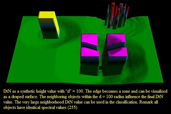
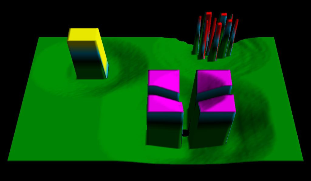
To demonstrate that the factor DtN is capable of classifying an image only by using the spatial layout, a synthetic image is created with solid square objects of similar spectral value. The original value equals 255 for all the pixel-objects and the largest squares are 130 × 130 pixels wide. The colors in Figure 1a express a classification result after processing of all initial white squares, solely according to similarities in the spatial layout. By only using the DtN-value, a density slicing with two values is applied, resulting in three different classes. Starting with DtN analysis for direct neighborhood, a double edge is returned. Both the Laplace filter and the DtN-value with “d” = 1 would show a result as displayed in Figure 1(b). This DtN value for “d” = 1 does not allow a segregation among all objects, only classifying background versus object (edge). By increasing the diameter of the search radius up to “d’ = 100, the contrasting edge now becomes a zone (see Figure 2), because neighboring objects within the radius influence the value for each pixel-object. These DtN values for large neighborhoods can be used to classify the single pixel-objects according to their spatial layout. Figure 2 shows the DtN value as a synthetic height value while the colors are the classification result for three different spatial classes using only thresholds. The background with negative values and a maximum of zero is displayed as a draped surface in green. This draping is a deformed surface as it matters to a single pixel-object what type of contrast exists within a “d” = 100 radius. Pixel-objects with similar spectral values residing inside the same square can receive their DtN value according to the effect of neighboring squares. This is not the case for all pixel-objects within one square. In Figure 2, part of the surface-pixels influenced by neighboring squares start to drop their DtN value. This is most visible on top of the 4 magenta squares which are deformed due to the influence of those neighboring squares. The conclusion remains that very large neighborhood analysis allows a classification on spatial context solely using the DtN value. Note that a classification is also possible after segmentation and defining the average size and distance to each neighboring object, which requires additional rules for aggregation. However, in this case the DtN value is assigned to each pixel, which avoids a compromise on segmentation settings. The importance of leaving out a decision on segmentation settings for pixel-object aggregation is crucial for further automatic processing. The need for an operator’s decision on segmentation settings adapted to every different satellite scene remains a bottleneck in full automatic analysis and if it can be postponed or extended it allows room for an increased automatic preprocessing in GEOBIA. Calibrating a potential aggregation setting according to initial DtN values for single pixel-object over large radii could be an important extension in finding compromises on further aggregation steps.
The result of the edge detection with DtN in Figure 1(b) should, in theory, be a similar double edge (one positive and one negative, see Figure 1(b)), in concordance with convolution as applied by the Laplace kernel but containing 1/4th of the Laplace filter (grey) value. Figure 2 shows the zonal result from a situation “d” = 100 producing a “donut”-like area, best visualized in the green background which subsides within the 100 pixel distance from a square.
3.2. Delineation of Fuzzy Objects
3.2.1. Density Slicing of Zones
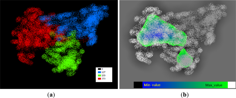
Density slicing on original spectral-values is sufficient as a trivial segmentation technique for crisp contrasting objects like the squares in Figure 1(a). The situation changes when there is no definite decision to be made on separating fuzzy objects. To illustrate the effect of fuzzy objects, three synthetic clouds are evaluated towards their behavior to a DtN equation. In Figure 3(a), three clouds with distinct grey-values 255 (red), 195 (green) and 127 (blue) are shown. There are zones where pixels with different spectral-values overlap. DtN values can be applied to set thresholds among these overlap zones as displayed in Figures 3(b) and 4(a,b). A color coding of the feature attributes ranging from black-blue (low) to green-white (high) are used here in an GEOBIA software environment.
After the calculation of contrast-values according to Equation (1) with “d” = 50, it is possible to use a visualization of high and low DtN values to express an area definition where similar DtN values are sharing similar spatial layout. The region with the highest contrast can be located which contains only objects with spectral values 255 and 0. There are also regions with intermediary and low contrast zones. The highest DtN-values are achieved by pixel-objects belonging to the red cloud with spectral value 255 (Figure 3(a)). After calculating DtN, the value equals or is lower than 255. If a single pixel object with spectral-value 255 is completely surrounded by 7,853 black pixels (502 × π) it would also receive a DtN value of 255. When other pixels-objects with spectral-value 255 are inside the search radius, this DtN value will be reduced. A pixel of spectral-value 255 surrounded by 7,853 identical spectral-value neighbors will receive a DtN value of 0.
Starting with the lowest DtN values (blue) in Figure 3(b), applying a threshold at a maximum of −105 (displayed in green), the lowest part of the range is occupied with pixel-objects containing spectral-value 0 among objects with spectral-values +255. At DtN value below −105, two centers of highest contrast and intermediary contrast are visualized in blue-green color coding in Figure 3(b). Any increment larger than −105 would merge these two centers.
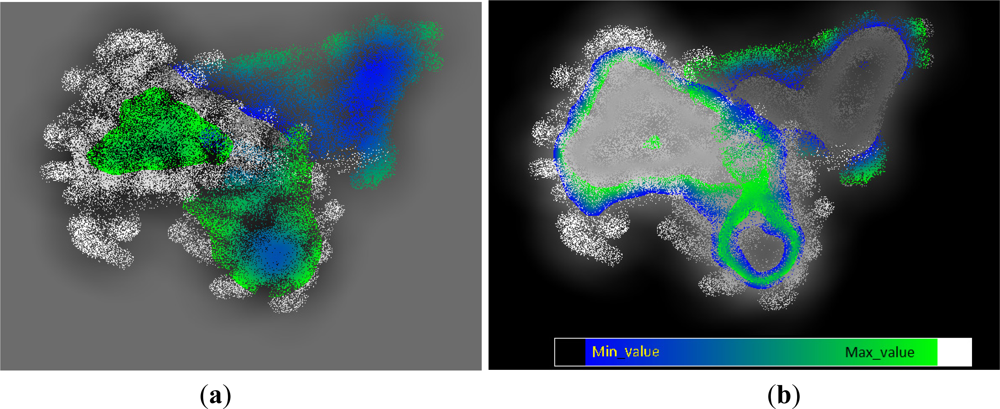
In Figure 4(a), a visualization of DtN value in the range 30–130 is chosen to display the zone where the clouds with spectral-values 127 (blue in Figure 3(a)) and 195 (green in Figure 3(a)) start to overlap. Contrary to Figure 3(b), where the color range displays the DtN-values for objects with spectral-value 0, Figure 4(a) displays the DtN values for objects with positive spectral-values.
Both Figures 3(b) and 4(a) contain negative DtN values where original spectral-values were 0. By making the DtN values absolute (modulus) as displayed in Figure 4(b), it becomes clear that the DtN values in a selected range can be used to create a zonal definition. The area with the highest positive DtN values also has the lowest negative DtN values that now “swap” sign in the display of absolute value of Figure 4(b). The range from 80 to 105 in Figure 4(b) is selected in such a way that the blue color close to the DtN value 80 is showing the overlap zone, indicating that a decision zone can be defined to split the overlap zone of the three clouds in three segments.
To emphasize this separating possibility, the isoline 60–65 is shown in Figure 5(a), where the zone can be found to split the two highest contrasting clouds from the lowest one.
In the overlap zones of the three clouds there is no undisputed decision to be made where to delineate the borderline between these clouds. The main decision to be made for Figure 3(a) is the boundary that splits the image in 3 areas where the spectral-value 255, 195 or 127 is dominant. In Figure 4(b), the visualization indicates that DtN value can also be applied with an absolute value around 80 but the exact chosen value is rather arbitrary. Using 60 as the threshold in Figure 5(a) is also a valid decision.
As mentioned before, “contextual information is needed to differentiate between areas with identical spectral response but different neighborhood characteristics”. The DtN value for large distances of “d” is solely responsible in incorporating this contextual information without the need of aggregating (segmenting above the single pixel level) of a local population of pixels which differ in size and distance to neighbors. Assigning a DtN value to single pixel objects is enough. To visualize this change from spectral value into DtN value, Figure 4(b) is displayed in a value range a lot larger than zero (chosen 80) and less than 130, considering 127 being the lowest spectral-value for cloud pixel-objects. Figure 4(a,b) displays zonal areas with near-similar values, clarifying that if the neighborhood is similar, neighboring DtN values will be similar too. For the pixel objects with 255 and 0 as spectral-value neighbors, on the left cloud (red in Figure 1(a)), it is less complicated than in the overlap zones of the three clouds. In the center of a cloud, due to their density, pixel-objects have identical grey values and their DtN values will be very low, reaching 0. This explains the donut-like centers of the clouds. The resulting “donut zones” are very different area delineations, as those resulting from a popular multiresolutional segmentation algorithm (cf. [10]), as used in eCognition (Figure 5(b)).
3.2.2. Comparing non-Competing Algorithms
There is no need to pose the question concerning which area delineation or segmentation algorithm is “better” as displayed in Figure 5(a,b). There is no arbitrary delineation to be made in the transition-zone between the clouds. No “best-reference” can be created for this situation and the answer as to which algorithm is best for area separation can therefore not be answered. What remains important is the ability to make comparisons between a simple DtN calculation and any other sophisticated segmentation algorithm. For a GEOBIA analysis, both approaches allow a good combination of feature attributes in a sequential segmentation process, where neither a single segmentation nor a single classification rule will provide a final result. It is the sequence [11] of essential segmentation-classification steps that lead to a satisfying classification. Thus, instead of aiming for the best segmentation algorithm, the focus should shift to a comparison of segmentation algorithms against some basic and simple area delineations, accompanied by an explanation of where and why they differ. The DtN-based area separation is a candidate to start the comparison due to its simplicity.
3.3. An Example with the Red Band of RapidEye
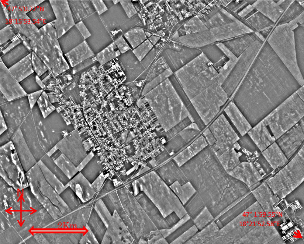
The synthetic imagery in Sections 3.1 and 3.2 can be used to understand the effect on objects with very similar spectral properties. The same effect observed in these experiments can be used to explain DtN effects on satellite imagery, especially in the task of artificial area detection. In Figure 6, a snapshot of Polgárdi near the city of Székesfehérvár, Hungary, is shown in RapidEye 5-m pixel size, which exists as a national mosaic. For artificial area extraction, 35 tiles of 255 tiles over Hungary where processed. The example presented in Figure 6 is a subset of nearly 30 km2 of a single 24*24 km tile.
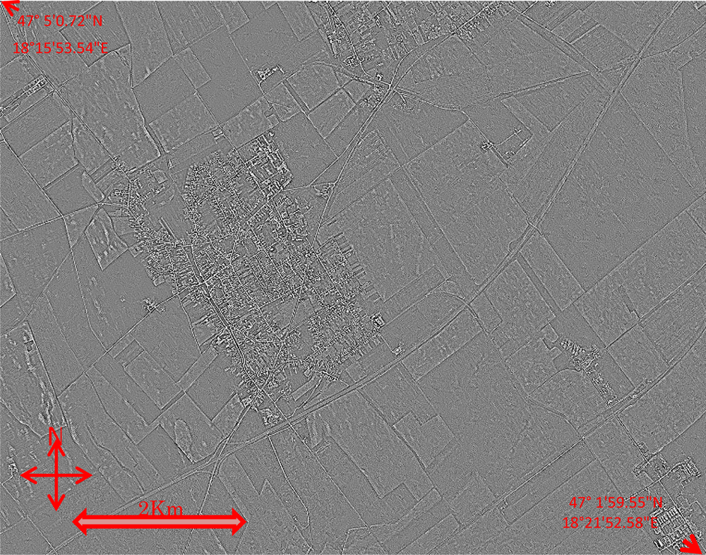
In Figures 7 and 8, the DtN is applied on the red band of RapidEye. At “d” = 1, the contrast-image resembles an edge-extraction result (Figure 7). At “d” = 25, the search area covers around 5 ha (Figure 8). At this scale, the initial edge detection becomes “zonal’ and is influenced considerably by the local land cover types in the imagery. Artificial image objects return the highest DtN values and their role is incorporated in the production of the artificial area vector of Figure 9. The open soil in Figure 6 contains bright spots as well as contrast. Because spectral values of open soil overlap the spectral signature of artificial areas, spectral analysis alone risks the establishment of commission failures by labeling open soil as settlement structure. Figure 10 repeats the same content of Figures 6–8 on a more detailed subset from the same 24*24 km tile. The main goal is to make sure that the open soil should be separable from artificial areas using the additional DtN values. A simplified protocol enables a basic extraction of artificial areas, as shown in Figure 9. This small five line protocol (in Figure 11) is the core of a more extensive classification developed especially for agricultural parcels outside of the scope of this paper. The five lines need extension in the agricultural domain in order to remove commission failures which are still part of the result in Figure 9. After visual inspection of the KMZ file draped over a GoogleEarth™ background of such a result as displayed in Figure 9, it is possible to use the 5 m pixel size in general for the artificial area extraction. This could reach details often up to single building detection at the national scale. This would be of advantage for classifying large area mosaics.
3.4. Extracting Artificial Areas
3.4.1. Visual Confirmation on GoogleEarth™
The context of the contrast mapping using DtN in this study has the status of an intermediary product. Although DtN is considered an important feature attribute in producing the polygon on artificial areas as displayed in Figure 9, the result will be clipped for agricultural parcels only. The use of the feature attribute DtN is part of an ongoing study on anomaly detection inside agricultural fields at the author’s institute. This will be further used to flag registered agricultural parcels which might have non-agricultural coverage. This part of the study requires extensive reference from visual interpretation for which accuracy assessment as yet cannot be given.
The achieved intermediary results (Figure 9) can be draped as KMZ files over a background, and in general visually confirm settlement layout. This is sufficient to define the aim of this study in the stratification of agricultural parcels where an accuracy analysis is pending. It is to be expected that the reader has access to free download and training versions of GEOBIA software. This would be an encouragement to repeat the presented process on the reader’s own data, in order to verify its usefulness by applying the DtN on a variety of values for “d” and drape the result over GoogleEarth™. The chosen artificial examples demonstrate that DtN values can be used to separate spectrally identical classes with different neighborhoods, as well define a zonal region when sharp contrasting edges are lacking. This allows comparison with segmentation algorithms of choice in a further aggregation.
3.4.2. A Simplified Protocol
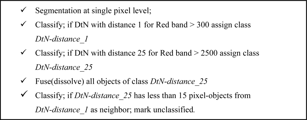
The values generated for DtN with different distances of “d” take into account the effect of self-repeatability and building patterns inside artificial areas. This is related to the scale of observations which is expressed here in the value for “d” using a 5 m resolution satellite mosaic. The initial application of “d” = 1 and “d” = 25 for 5 meter pixels is a first step. On very large self-repetitive patterns like huge chessboard patterns, any radius will return the same result. Deviations from self-repeatability will stand out as a result of this calculation (anomaly detection). The optimal values of “d” could be related to a stratification beforehand with or without the assistance of additional thematic information. The effect of the different spectral bands is important but requires more insight, especially in the red-edge spectrum (band 4 in RapidEye). To demonstrate its use, Figure 11 displays the rule set used for Figure 9 starting with the red spectral band.
Figure 11 displays the 5 decision lines to create the artificial area polygon of Figure 9. After a single-pixel object segmentation, the two classes are created for DtN, “d” = 1 (DtN_distance _1) and DtN, “d” = 25 (DtN_distance_25). For both features, the highest contrast is used with thresholds 300 and 2,500 (16 bit image input, values depending on RapidEye original spectral values). The contrast for “d” = 25 corresponds to large buildings and open soil patches. After object-fusion of this class (DtN_distance_25) the fused object having less than 15 pixel-objects of high contrasting neighbors at “d” = 1 will be marked unclassified. This removes most of the open-soil patches which lack abrupt contrast changes for “d” = 1.
This rule set demonstrates the possibility to start a detection of a certain group of contrasting pixels. It removes many open soil patches from the contrasting objects because they do not have so many contrasting single-pixel objects as direct neighbors in comparison with industrial buildings, farms and open mine pits. This rule set is incomplete while many commission errors are still present, but it is still a good demonstration of the function of DtN in the total rule set. Extensions of the rule set concentrate further on the reduction of commission failures. With these five lines it can already be demonstrated that the large amount of artificial areas in RapidEye mosaics can be detected and a visual drape of this result will allow confirmation on a high resolution background. The reader is therefore recommended to apply the rule set lines on his own dataset and repeat the GoogleEarth™ drape. Aggregation on higher levels in a GEOBIA environment is recommended to finalize the complete artificial area detection.
3.5. Hardware and Technical Specifications
The rule set is only a core part of a larger RapidEye processing series. The calculation of DtN with value “d” = 25 is responsible for the largest part of the processing time. The specifications of the total project are given here to highlight the fact that the use of DtN is not only a theoretical concept but can also be implemented practically in large mosaic processing of satellite data. For the overall project of 35 tiles, and a rule set much larger than the example in Figure 11, a single PC, based upon an i7 processor with 12 GB DDR-3 RAM, needs around 80 hours to process 80GB of RapidEye imagery. The original 5 spectral bands of RapidEye were extended with 3 artificial bands made up of additional “tassled cap brightness” and two alternative edge detection bands for testing purposes. This explains why 35 tiles of RapidEye data reach 80 GB. An image tiling of 24*24 km is applied. The derivatives mentioned play a role in further commission error removal outside the scope of this paper. A single tile could be processed in ±15 min without using DtN. The use of DtN (with d = 25) forces the process requiring more than 2 h per tile, applying the feature in several decision lines. The total processed area is around 20,000 km2 at 5 m pixel size, fit for 1:25,000 mapping scale. The experience so far is that the incorporation of the DtN for various “d” allows the application of a single protocol over the complete mosaic without changing the classification rules. The transfer from absolute spectral values to relative contrast values already contributes in the application of a single master protocol for all tiles. The absolute spectral values depend on seasonal changes and atmospheric conditions. The relative contrast values are less affected by these changes.
4. Discussion
4.1. Preserving Information before GEOBIA Aggregation
The study focuses attention on an additional preprocessing step based on contrast among single pixel objects. Although a simple procedure, the applied equation is resource intensive and evaluates the contextual information for pixels at close and far neighborhoods. The procedures can be implemented by users with access to robust hardware capacity. The central equation (see Equation (1), Section 3.2) is focused on the mean difference (of spectral value) to neighborhood. Some steps in the application of the feature attribute “Mean Difference to Neighbor” are not self-evident:
- The GEOBIA focus on the classification of local homogeneous pixel populations [1,12]. The first step in GEOBIA analysis normally concentrates on segmenting useful image objects containing local pixel populations with a mean value and standard deviation. A deviation of this standard practice is suggested in order to preserve the feature attributes of single pixel objects.
- In the selection of useful feature attributes for GEOBIA classification, there is no suggestion on the optimal setting for the diameter search radius in DtN. This paper recommends the inclusion of large neighborhood analysis in addition to common contrast analysis on local neighborhoods.
- The radius “d” = 25 for satellite imagery with 5-m pixel size is chosen to obtain a result in a matter of 10 to 15 min for each calculation but “d” = 50 or “d” = 100 could be useful if extensive hardware resources are available. The design of feature attributes in this respect remains a problem to be solved by expert design based upon domain knowledge.
- DtN values for single pixels with large “d” search radius must explicitly be set as a parameter. Offering a large set of features to an automatic feature mining procedure risks that only the direct neighborhood of DtN using low values for “d” will be evaluated and the advantages of large neighborhood for DtN are then at risk of being neglected.
- The characterizing of a single value for radius “d” is not sufficient for the context of a single-pixel object, but a series of values for close and far neighborhoods is required. The optimal sequence is part of ongoing research.
4.2. Agricultural Application with Urban Mapping Extensions
The use of the DtN for large areas within this study aims at detecting anomalies in agricultural databases within selected parcels. The development aims at an application at the national scale using automatic anomaly detection for each growing season. The agricultural management in European conditions largely depends on the use of agricultural machinery. This causes a relative homogeneous layout of agricultural parcels for major seasonal crop types and permanent grasslands. The DtN analysis over small and large neighborhoods is sensitive to areas in the image where contrast can be linked to non-agricultural use inside homogeneous parcels. The intermediary results are visualized over publicly available large scale imagery such as the GoogleEarth™ backdrop. This visual check shows that the large response to DtN contrast analysis exists outside the registered and evaluated agricultural area and follows the layout and distribution of urban fabric at the national scale. Figure 9 visualizes the response to DtN analysis which confirms the origin of the responses due to contrast caused by the layout of single buildings within settlements and cities. Moreover, it is the large area availability of the vector layout which makes pre-processing with DtN noticeable. The raw contrast sketch that is only partially displayed in Figure 9 is available in this study for more than 20,000 km2, and can be extended to the whole country.
Building detection that exceeds many thousands of target objects over large areas is possible. However, according to Shorter and Kasparis, the recent studies in this domain generally present much smaller classified areas [13]. This is partly due to limited available coverage of seamless sub meter satellite data which remains rare at the national scale. Satellite data at sub meter resolution is mainly available as patches or parts of mosaics. Experiences in the application of the DtN in building detection on very high resolution imagery with 50-cm pixel size confirms its usefulness in artificial area detection and leads to 0.3% omission and 13% commission errors on artificial area detection on selected tiles with ±250 buildings per km2. This example was created from a mosaic of 3 GeoEye images on a total area of 80 km2 [14]. National coverage at seasonal interval remains a challenge for satellite imagery with sub 1 meter pixel size, due to its limited availability as a seamless mosaic. The sub 5-m pixel size might lead to better individual building detection, but the large area coverage of settlement layout makes DtN analysis attractive in national mosaics using a 5-m pixel size.
Mechanization within agricultural fields in Europe results in spectral homogeneity within parcels. Objects with high contrast are expected to be a rare phenomenon in those parcels. A proper accuracy assessment would focus on the majority of parcels not containing anomalies and parcels with a correct anomaly detection that is related to an area of non-agricultural use. While this evaluation part of the study is pending, the visualized results of a pre-processing stage in GEOBIA reveal that the information on contrast in single pixels is important. Urban analysis and artificial area detection has been part of GEOBIA at a variety of scales [12]. There is a risk if GEOBIA focuses initially on segments of homogeneous pixels, thus aggregating image objects first. As the proposed pre-processing comes in addition and not as a replacement for the suggested procedures in Blaschke et al. [12], the aggregation remains valid while integrating the important feature attribute of single pixel objects at the lowest GEOBIA level and using the properties at higher aggregation levels. Urban mapping and single building detection is a common topic in GEOBIA [15], and the use of convolution and edge detection is regarded amongst the more important features in building detection [16]. The equation presented extends the already available list of features where the ability to apply the analysis to very large neighborhoods is related to a trend in the availability of increased hardware capacities. This is in addition to recent approaches in the domain of building detection that discuss the applications of edge detection and contrast analysis using limited window size on smaller neighborhoods only [16].
4.3. Potential for Additional Applications of DtN
The experimental section with synthetic data shows that large neighborhood contrast with DtN allows both classification as well as area delineation, based upon density slicing of a single value. The technique might not lead to the most applicable result but can certainly be used in calibrating alternative area delineating techniques and the characterization of areas of the same class in order to compare and adapt alternative GEOBIA strategies. The most promising role lies in automatic directing of homogeneity factors for segmentation in order to avoid interactive training of reference objects requiring digitizing on screen to train the segmentation algorithm settings [15]. The visual delineation as input will probably follow the outside walls of buildings and those are the pixel objects that have a high DtN response. This is most obvious in Figure 9 for industrial complexes. Here the DtN analysis delivers a vector that contains size and amount of objects standing out on a larger scale. These properties on size and amount or density can be used to guide segmentation settings in those areas. From Section 3.2.1, the DtN values allow a conclusion to be drawn that distinct regions exist in the image which can be used to design segmentations settings for large object aggregation. The results of a DtN analysis can be seen as preparing a seedbed with contrasting objects that give directions on size and homogeneity criteria for further GEOBIA aggregation. The distribution of the size of large buildings in Figure 9 can already be used to estimate segmentation parameters for a new segmentation round.
Another potential development is the use of specific edge classification. This remains a rare topic in image analysis [17]. The series of DtN values for single pixel objects can be used to characterize sharp and smooth transitions and allow differences among edge characteristics to be expressed. The isolines of Section 3.2.1 already indicate this potential, where Section 3.1 describes edges that are part of a staircase type of edges leading to a plateau. The GEOBIA information could thus elaborate the work from Chidiac and Ziou [17], with additional information on large neighborhood characteristics of aggregated objects using the expansion of the hardware resources which have since become available.
The ongoing assessment of accuracy for agricultural parcels should not hinder the presentation of an intermediary step as presented in this paper. The national settlement structure or “urban fabric” is an unexploited side effect of the study. The application of the equation presented might be more important for military mapping standards such as V-Map updating for organizations like NGA/NIMA, where GEOBIA and textural analysis using low-homogeneity for urban applications already could show automatic results [18]. The equation is especially suited for detection of large single buildings and the overall settlement layout at the national scale. This does not require a 100% building detection. Also, an extension of full automatic CORINE/CLC [19] land cover update would require a different area definition for urban fabric, should the single building analysis and artificial-area pattern distribution become part of the CLC class definition.
5. Conclusions
Starting a Geographic Object Based Image Analysis (GEOBIA) session has the habit or “best practice” of setting segmentation parameters in order to establish homogeneous image objects. This paper recommends changing this habit and integrating a pre-processing step at the level of single pixel objects. GEOBIA changes the properties of contrast for image objects at every level of segmentation/aggregation. Because of the essential segmentation step in a GEOBIA procedure, the detailed feature attributes at the single pixel level are at risk of being neglected. However, the feature attributes for single pixel objects should be made available to classification steps at higher levels of object aggregation. It is recommended that contrast at the pixel object level should be analyzed using the presented equation on mean difference to neighbor (DtN) for close neighborhoods, but certainly also for larger ones, before further object aggregation.
The synthetic experiments show that a single value for DtN on large neighborhood contrast can be used for area delineation as well as classification applying only density slicing. To reach such results, a very limited number of decisions has to be made. This offers a direction towards automatic analysis with a minimal amount of user input and in the first place avoids a compromise on segmentation settings that are essential in GEOBIA. This strategy aims to rely less on trial and error procedures in finding segmentation settings but rather to follow suggestions for parameter settings (for segmentation) guided by area size, amount and density of structures that remain outstanding in the image after DtN analysis.
The proposed method was developed for anomaly detection in agricultural parcels. The visualization over very large areas outside agricultural parcels indicates that it is the layout of single buildings that are responsible for the appearance of objects with positive response to DtN analysis. The detection of every single building is not crucial here, but the overall layout of villages and towns at national scale becomes accessible. A better single building detection in VHR satellite data is unlikely to cover a country. The need for country-wide mapping of artificial areas is pressing and the proposed equation can be evaluated as part of a pre-processing step using freely available data and software. This will facilitate the interested user to repeat the suggested application of DtN analysis, especially for very large neighborhoods, providing high performance hardware is available.
The use in the agricultural domain for this intermediary product is limited and accuracy analysis in the agricultural domain requires an extension of the classification with GEOBIA in addition to the DtN analysis. Nevertheless, the approach is applicable to other domains involving artificial area detection. At present, only limited information on the accuracy analysis of this approach can be given, mainly based on visual interpretation of GoogleEarth™ overlays. The goal of single building detection lies at the edge of the feature extraction possibilities in satellite imagery with 5 meter pixel size.
Acknowledgments
I would like to thank Lewinski, S. and Hejmanowska, B. for their critical remarks and useful suggestions during the development of this application.
References and Notes
- Blaschke, T.; Lang, S.; Hay, G.J. (Eds.) Object Based Image Analysis; Springer: Heidelberg/Berlin, Germany, 2008.
- Gorte, B. Multi-spectral quadtree based image segmentation. Int. Arch. Photogramm. Remote Sens 1996, 31, Part B3,. 251–256. [Google Scholar]
- Burt, P.J.; Adelson, E.H. The Laplacian Pyramid as a compact image code. IEEE Trans. Commun 1983, 31, 532–540. [Google Scholar]
- Walter, V. Object-based classification of remote sensing data for change detection. ISPRS J. Photogramm 2004, 58, 225–238. [Google Scholar]
- Marr, D. Vision; Freeman Publishers: New York, NY, USA, 1982. [Google Scholar]
- Dykes, S.G.; Zhang, X. Folding Spatial Image Filters on the CM-5. Proceedings of 9th International Parallel Processing Symposium, Santa Barbara, CA, USA, 25–28 April 1995.
- Wijaya, A.; Marpu, P.R.; Gloaguen, R. Geostatistical, Texture Classification of Tropical Rainforests in Indonesia. Proceedings of 5th International Symposium in Spatial Data Quality, Enschede, The Netherlands, 13–15 June 2007.
- Trimble/Definiens. Definiens, eCognition Developer 8.1, Reference Book, Accompany Version 8.1.0; Build 1653 x64, 17 September 2010. (Part of the software installation package).
- Horne, J.H. A Tasseled Cap Transformation for IKONOS Images. Proceedings of ASPRS 2003 Conference, Anchorage, AK, USA, 4–9 May 2003.
- Baatz, M.; Schaepe, A. Multiresolution Segmentation—An Optimization Approach for High Quality Multi-Scale Segmentation. In Angewandte Geographische Informationsverarbeitung XII; Strobl, J., Blaschke, T., Griesebner, G., Eds.; Wichmann Verlag: Karlsruhe, Germany, 2000; pp. 12–23. [Google Scholar]
- Zhang, R.; Zhu, D. Study of land cover classification based on knowledge rules using high-resolution remote sensing images. Expert Syst. Appl 2011, 38, 3647–3652. [Google Scholar]
- Blaschke, T.; Hay, G.H.; Weng, Q.; Resch, B. Collective sensing: Integrating geospatial technologies to understand urban systems—An overview. Remote Sens 2011, 3, 1743–1776. [Google Scholar]
- Shorter, N.; Kasparis, T. Automatic vegetation identification and building detection from a single nadir aerial image. Remote Sens 2009, 1, 731–757. [Google Scholar]
- de Kok, R.; Tasdemir, K. Contrast Analysis in High-Resolution Imagery for Near and Far Neighborhoods. Proceedings of GEOBIA 2012, Rio de Janeiro, Brazil, 7–9 May 2012; pp. 196–200.
- Novack, T.; Esch, T.; Kux, H.; Stilla, U. Machine learning comparison between WorldView-2 and QuickBird-2-simulated imagery regarding object-based urban land cover classification. Remote Sens 2011, 3, 2263–2282. [Google Scholar]
- Tarantino, E.; Figorito, B. Extracting buildings from true color stereo aerial images using a decision making strategy. Remote Sens 2011, 3, 1553–1567. [Google Scholar]
- Chidiac, H.; Ziou, D. Classification of Image Edges. Proceedings of Vision Interface ’99, Trois-Rivieres, QC, Canada, 19–21 May 1999; pp. 17–24.
- Leukert, K. Übertragbarkeit der Objektbasierten Analyse bei der Gewinnung von GIS-Daten aus Satellitenbildern Mittlerer Auflösung. University of the German Federal Armed Forces, Munich, Germany, 2005. [Google Scholar]
- Bossard, M.; Feranec, J.; Otahel, J. CORINE Land Cover Technical Guide; Addendum, EEA: Copenhagen, Denmark, 2000. [Google Scholar]
Figure 1.
(a) Simulation of a classification with squares of similar spectral value but different spatial layout and (b) their “DtN” edge detection for “d” = 1. This edge detection should theoretically be in concordance with the result of Laplace convolution and should be similar for close neighborhood. The DtN values for “d” = 1 cannot be used to classify the differences in spatial layout.
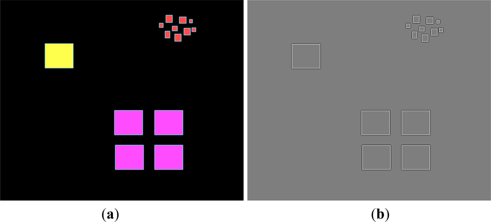
Figure 2.
DtN as a height value with “d” = 100 applied on Figure 1(a). The edge becomes a zone. The neighboring objects within the d = 100 radius influence the final DtN value. Contrary to Figure 1(b), the very large neighborhood DtN value can be used in the classification.
Figure 2.
DtN as a height value with “d” = 100 applied on Figure 1(a). The edge becomes a zone. The neighboring objects within the d = 100 radius influence the final DtN value. Contrary to Figure 1(b), the very large neighborhood DtN value can be used in the classification.

Figure 3.
(a) Three clouds with grey-values 255(red), 195(green) and 127(blue), and (b) showing all negative contrast-values < −105 for pixel-objects with spectral value 0.
Figure 3.
(a) Three clouds with grey-values 255(red), 195(green) and 127(blue), and (b) showing all negative contrast-values < −105 for pixel-objects with spectral value 0.

Figure 4.
(a) Zones of near equal values. Range 30–130. (b) Combining Figure 3(b) and 4(a) by making all contrast values absolute (modulus). Range 80–105.
Figure 4.
(a) Zones of near equal values. Range 30–130. (b) Combining Figure 3(b) and 4(a) by making all contrast values absolute (modulus). Range 80–105.

Figure 5.
(a) The isoline 60–65 for absolute DtN value, (b) A multiresolutional segmentation result for comparison.
Figure 5.
(a) The isoline 60–65 for absolute DtN value, (b) A multiresolutional segmentation result for comparison.
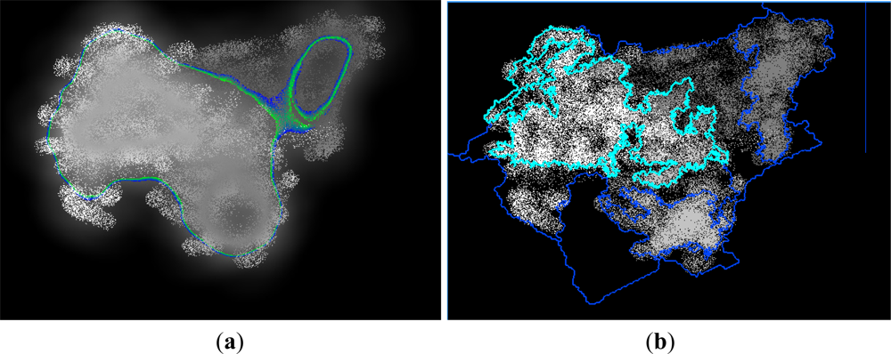
Figure 6.
Detail of 30 km2 from a 24*24 km tile of the village Polgárdi, Hungary, red band of a subset of RapidEye (circa 20 km2).
Figure 6.
Detail of 30 km2 from a 24*24 km tile of the village Polgárdi, Hungary, red band of a subset of RapidEye (circa 20 km2).

Figure 7.
Contrast for “d” = 1 (in Equation (1)) on the red band.

Figure 8.
Using DtN with “d”= 25 pixel radius.

Figure 9.
Part of artificial area extraction as GIS polygons on Polgárdi, similar area as Figure 6.
Figure 9.
Part of artificial area extraction as GIS polygons on Polgárdi, similar area as Figure 6.
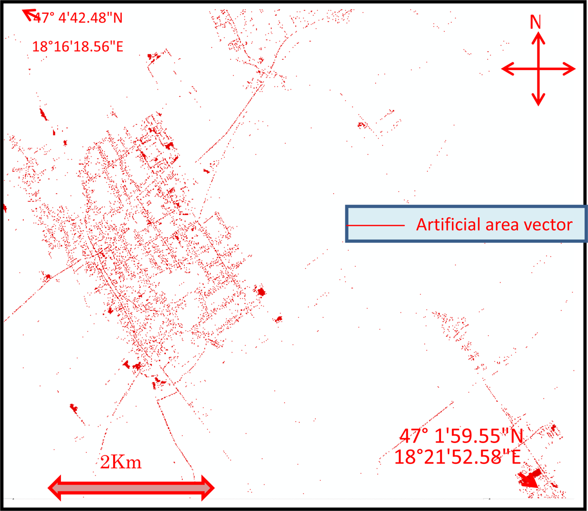
Figure 10.
Detail from the same tile used for Figures 6–8. (a) red band RapidEye, (b) d = 1, (c) d = 25.
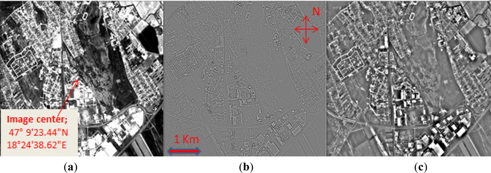
Figure 11.
The rule set to create Figure 9.
Figure 11.
The rule set to create Figure 9.
Share and Cite
MDPI and ACS Style
De Kok, R. Spectral Difference in the Image Domain for Large Neighborhoods, a GEOBIA Pre-Processing Step for High Resolution Imagery. Remote Sens. 2012, 4, 2294-2313. https://doi.org/10.3390/rs4082294
AMA Style
De Kok R. Spectral Difference in the Image Domain for Large Neighborhoods, a GEOBIA Pre-Processing Step for High Resolution Imagery. Remote Sensing. 2012; 4(8):2294-2313. https://doi.org/10.3390/rs4082294
Chicago/Turabian StyleDe Kok, Roeland. 2012. "Spectral Difference in the Image Domain for Large Neighborhoods, a GEOBIA Pre-Processing Step for High Resolution Imagery" Remote Sensing 4, no. 8: 2294-2313. https://doi.org/10.3390/rs4082294