Article

Monitoring Seasonal Hydrological Dynamics of Minerotrophic Peatlands Using Multi-Date GeoEye-1 Very High Resolution Imagery and Object-Based Classification

1
INRS, Centre Eau Terre Environnement, 490 rue de la Couronne, Québec, QC G1K 9A9, Canada
2
Centre d’Études Nordiques (CEN), Pavillon Abitibi-Price, 2405, rue de la Terrasse, Local 1202, Université Laval, Québec, QC G1V 0A6, Canada
*
Author to whom correspondence should be addressed.
Remote Sens. 2012, 4(7), 1887-1912; https://doi.org/10.3390/rs4071887
Submission received: 28 April 2012 / Revised: 19 June 2012 / Accepted: 20 June 2012 / Published: 26 June 2012

Abstract

:
The La Grande River watershed, located in the James Bay region (54°N, Quebec, Canada), is a major contributor to the production of hydroelectricity in the province. Peatlands cover up to 20% of the terrestrial environment in this region. Their hydrological behavior is not well understood. The present study is part of a multidisciplinary project which is aimed at analyzing the hydrological processes in these minerotrophic peatlands (fens) in order to provide effective monitoring tools to water managers. The objective of this study was to use VHR remote sensing data to understand the seasonal dynamics of the hydrology in fens. A series of 10 multispectral pan-sharpened GeoEye-1 images (with a spatial resolution of 40 cm) were acquired during the snow-free season (May to October) in 2009 and 2010, centered on two study sites in the Laforge sector (54°06′N; 72°30′W). These are two fens instrumented for continuous hydrometeorological monitoring (water level, discharge, precipitation, air temperature). An object-based classification procedure was set up and applied. It consisted of segmenting the imagery into objects using the multiresolution segmentation algorithm (MRIS) to delineate internal structures in the peatlands (aquatic, semi-aquatic, and terrestrial). Then, the objects were labeled using a fuzzy logic based algorithm. The overall classification accuracy of the 10 images was assessed to be 82%. The time series of the peatland mapping demonstrated the existence of important intra-seasonal spatial dynamics in the aquatic and semi-aquatic compartments. It was revealed that the dynamics amplitude depended on the morphological features of the fens. The observed spatial dynamics was also closely related to the evolution of the measured water levels.

1. Introduction

Hydroelectricity production in the province of Quebec is highly dependent on the hydrological conditions of the Mid-Northern region. The hydroelectric complex on the La Grande River covers a watershed of more than 177,000 km2 [1]. The eight dams currently present on this river alone generate around 40% of the hydroelectricity in Quebec [2]. Since 1985, the water levels in these reservoirs have varied dramatically for reasons not currently understood [3]. One hypothesis involves variations in the storage of water by peatlands, which are strongly represented in the watershed.
Peatlands, characterized by an accumulation of over 40 cm of peat [4], represent over 90% of Canadian wetlands [5]. They occupy about 20% of the terrestrial environment of the watershed of the La Grande River [6]. In this region, peatlands are mostly patterned, with alternating pools and vegetated strings. Previous studies have demonstrated that this fine-scale topography strongly influences the water balance of the peatland by reducing or delaying runoff, leading to the temporary storage of water in pools [7], and by increasing evapotranspiration and water storage capacity [8]. The buffer effect of peatlands (both bogs and fens) is inversely proportional to the water table level [911]. Strong seasonal variations of flow characterize peatlands. They generally have their maximum flows during the snow melt season, while the flow can be zero during long dry periods in the summer [12].
In the past decade, there has been increasing interest in the use of remote sensing science to map wetlands and monitor their hydrological changes [13]. However, wetlands are inherently difficult to map: their boundaries exist along a wetland/upland continuum, and they are subject to regular changes in inundation that result in complex assemblages of vegetation and habitat types [14].
Originally, due to the limited spatial resolution of optical and radar sensors (10–30m), studies focused on discrimination and inventorying of wetlands [1517]. More recently, remote sensing has been used to study ecological and hydrological aspects of wetlands [1822]. Aerial photographs were recently used to study the dynamics of peatland pools in the La Grande River watershed at a multi-decadal scale [23]. The results showed that these pools are very sensitive to climate conditions, their size varying according to climate change.
The emergence of new satellite sensors providing very high spatial resolution images (VHR) has raised new hopes for environmental and urban monitoring [2426]. These images provide an attractive alternative to aerial photographs due to short satellite return intervals and digital data formats easily integrated into geographic information systems [13]. Recent studies have shown that VHR imagery is suitable for the detailed mapping of temporary water bodies at a local scale [26,27]. Dissanska et al. [26] developed a semi-automated approach for assessing the spatiotemporal development of terrestrial and aquatic compartments in patterned peatlands of the La Grande River watershed based on very high resolution panchromatic images. This study, which operated at a multi-decadal scale (1957–2006), proposed a robust method of classification with an overall accuracy of 81% that was able to detect significant changes in the aquatic areas of the studied peatlands.
These studies suggest that VHR multispectral imagery might be a good tool for monitoring the hydrological behavior of patterned fens, with the help of an object-based classification approach including specific rulesets. Our study covered two seasons (2009 and 2010) and involved comparison of imagery-derived statistics (through classification) with in situ hydrometric measurements. The results should help water managers to better model the specific hydrological regime of fens.
This study had three objectives: (1) Test the potential of VHR multispectral images to delineate and classify the internal structure of the peatlands. (2) Use VHR imagery to verify the existence of seasonal dynamics of aquatic and semi-aquatic structures in patterned fens and quantify these dynamics. (3) Determine if the observed dynamics can explain the hydrological regime of fens.

2. Material and Methods

2.1. Study Area

The study area is located in the middle part of the La Grande River watershed in the James Bay region (Quebec, Canada), 15 km south of the Laforge 1 hydroelectric dam (Figure 1). The region is characterized by a relatively flat relief. Woodlands with lichen and black spruce, lakes, and patterned fens prevail in the landscape. Climatic conditions are subarctic, with temperatures that range from −35 °C (January) to +20 °C (July), a mean annual temperature about −4.2 °C, and mean annual precipitation around 830 mm. The growing season is about 119 days long [28]. Two sub-basins were chosen based on their high proportion of water surface on the fens, their relatively easy access from the road, their small size, and their well-defined boundaries [29].
The site 1 watershed (54°06′52″N, 72°30′02″W) has an area of 12.1 ha. This catchment area (Figure 1) was determined by a digital elevation model created from a grid of DGPS surveyed points [29]. The watershed contains a fen (31%) and a section of forest-covered land (69%). The fen, split into two wings, is patterned with a succession of elongated pools and narrow ridges that eventually discharge into a larger pool near the outlet [29]. The main slope of the fen was estimated to be 1.45% [29]. The fen is connected to a lake downstream by a single outlet with an elevation of 439 m above sea level.
The site 2 watershed (54°06′41″N, 72°30′56″W) has an area of 3.7 ha (Figure 1). The watershed contains a fen (51%) and a section of forest-covered land (49%). The fen is patterned mostly with a succession of wide pools and narrow ridges, along a single wing. The main slope of the fen was estimated to 1.5%. The western part of the fen is connected to a lake upstream. The eastern part of the fen is connected to a lake downstream by a single outlet with an elevation of 437 m above sea level.

2.2. Hydrometeorological Measurements

Wells equipped with hydrostatic pressure gauges were installed on sites 1 and 2 in 2009 (Figure 2). The wells were made of PVC pipe with slots along the entire length. Water level data were collected every 15 min by the hydrostatic pressure gauges (leveloggers, Solinst, model 3001, accuracy ±0.3 cm, http://www.solinst.com/). On site 1, well A was installed in a saturated ridge. On site 2, well B was installed in a pool. The measurements were corrected for atmospheric pressure. To do this, a barometer from a weather station installed at site 1 was used (Campbell Scientific, 61205 V, R.M. Young, accuracy ±0.5 hPa, http://www.campbellsci.ca/). Temperature and precipitation were also measured by this weather station (Figure 2).
Two trapezoidal flumes (TRACOM, Large 60°V and SRCRC 12″ 45°V models, accuracy ±0.1%, http://www.tracomfrp.com/flumes.htm) were installed in 2008 at the outlet of site 1 (Figure 2). Water flows to the outlet between two rock bands that define a 15-m-wide corridor. A small weir was installed to ensure that the surface flow passed through a single outlet. The large flume (Flume A) was installed at the outlet of the weir to measure flood flows (1.4–220 L/s). The smaller flume (Flume B) was set 2 m downstream. It provided higher accuracy recording of the majority of seasonal flow (0.06–9.8 L/s). Both flumes were equipped with a stilling well. The water level in the well was measured every 15 min. Measurements were corrected for atmospheric pressure. The water levels were then transformed into flows (L/s) using rating curves supplied by the manufacturer [29].

2.3. Satellite Imagery

2.3.1. Acquisition

To study the seasonal dynamics of the hydrology of the fens, 10 VHR multispectral satellite images were acquired during spring and summer 2009 and 2010 (Table 1). These images were recorded by the GeoEye-1 (GeoEye, Inc) satellite sensor, providing panchromatic spatial resolution of 0.41 m (0.5 m pixel resampling) and RGB/NIR spatial resolution of 1.65 m (2 m pixel resampling). Due to the frequent cloud cover in the study area, only 4 images out of the 10 were without a significant presence of clouds.
Our first priority was to obtain images capturing the widest possible range of hydrological conditions, i.e., both very low and very high discharge events. This would have enabled us to cover the majority of the seasonal hydrological dynamics in the fens. However, we were unable to acquire images during periods of high discharge (Figure 3). Two major reasons explained this: cloud cover usually remains high when the discharge response to precipitation occurs (a few hours after the precipitation event), and the frequency and duration of high discharges are relatively low (Figure 3).

2.3.2. Preprocessing

The 10 images were georeferenced in the Universal Transverse Mercator (UTM) coordinate system, Zone 18 north, North American Datum for 1983 (NAD83). Every image was supplied with a mathematical model of the image geometry in the form of rational polynomial coefficients (RPC). Images were orthorectified using these RPCs and a DEM of the area at 1/50,000 scale, supplied by Geobase ( http://www.geobase.ca). Two accurate 3D ground control points were added to each image to improve orthorectification. This led to an accuracy of about a pixel size for each image channel, 0.5 m and 2 m for the panchromatic and multispectral channels respectively.
After these geometric corrections, radiometric calibrations were performed to standardize each image. First, digital number (DN) values were converted to at-sensor radiances using prelaunch gain and offset coefficients [30]. Then, at-sensor radiances were converted to at-sensor reflectances using the acquisition geometry following [31].
The panchromatic (0.5 m pixel resolution) and multispectral (2 m pixel resolution) channels of the images were then fused using the PCI Geomatics® pan-sharpening algorithm [32]. This algorithm was used because it produces good results without changing the statistical parameters of the original images [33]. The resulting “pan-sharpened” images retained the spectral features of the low resolution multispectral image while integrating the spatial details of the high resolution panchromatic image (0.5 m pixel resolution).
Many parameters (e.g., visibility, atmosphere composition) are needed to perform an absolute atmospheric correction of the satellite imagery to obtain surface reflectances from at-sensor reflectances. Unfortunately, we did not have the requisite data for these images. Thus, a multiple-date image normalization using regression was performed between a reference image and the remaining images [34].

2.4. Object-Based Image Classification

2.4.1. Procedure

An object-based classification procedure was set up and applied to delineate internal structures in the peatlands (aquatic, semi-aquatic, and terrestrial) using VHR multispectral imagery. This would enable the seasonal spatial evolution of the hydrology of the fens to be monitored. An approach by region (object-based image analysis) [35] was chosen because it uses not only the spectral information contained in the image but also spatial and topological information. The procedure was inspired by the semi-automated approach developed by Dissanska et al. [26] using panchromatic images at a multi-decadal scale.
The eCognition 8.64.0® software was used to build the procedure. A hierarchical approach was utilized to enable better adaptation to the diversity, complexity, and patterned structure of the natural ecosystems [36]. First, a coarse-scale analysis was performed on a reference image (9 June 2010) to delineate the major landscape units. A fine-scale analysis was then performed on the 10 images to create a classification map of the study sites. The scheme of the object-based analysis procedure is presented in Figure 4.
Multiresolution segmentation (MRIS) [37] was used in the study. MRIS is a region-growing segmentation algorithm that groups adjacent pixels to create objects (polygons) that later will be assigned to a class. These groupings are based on the internal heterogeneity criteria of the resulting objects, which cannot exceed a user-defined scale parameter. Higher values for the scale parameter result in larger image objects, and smaller values result in smaller ones [38]. The first and second principal component (PC) bands derived from the pan-sharpened imagery were used as input bands in the segmentation process. A weight was assigned to both input bands, reflecting the amount of variance of the initial four bands contained in the derived PC bands, i.e., more than 80% for PC1 and less than 15% for PC2. Regarding the coarse-scale analysis, a high scale parameter value of 30 was chosen to delineate the major landscape units (forest, water, peat...). To create homogeneous objects within the scene, weights of 90% for color and 10% for shape were used. This ratio was chosen because natural environments, with no specific shape, were being monitored. To specify the shape, a relationship of 70 to 30 between compactness and smoothness was selected. We expected that this segmentation would provide a good distinction between peatlands and forests. Regarding the fine-scale analysis, a scale parameter of 10 was chosen to precisely delineate the internal structures of peatlands. The same ratios as those used in the coarse-scale analysis were applied between the shape and color parameters and between the compactness and smoothness parameters.
Eco-hydrological classes were defined (Table 2), based on literature [26,3941] and knowledge of the field. Once classes are defined, classification rules have to be determined. Membership functions and the nearest neighbor algorithm are the main classification tools used in the eCognition software [38]. The nearest neighbor algorithm needs training sites. To improve separation between the defined classes by adding meaningful features in the nearest neighbor classification process, bands were derived from the pan-sharpened images. First, Intensity–Hue–Saturation (IHS) transformation of the RGB channels was undertaken [42]. Then the following band ratios and indices were calculated: Ratioblue (Blue/(Blue+Green+Red)) [36], Chlorophyll Index ((Red/Green)–1) [43], and NDVI index ((NIR–Red)/(NIR+Red)) [44]. Textures, often used as an additional tool for wetland mapping, were also calculated [16,26]. However, tests of these features showed that the NDVI and textures channels did not provide any improvement in the discrimination of classes.

2.4.2. Classification Accuracy Assessment

Classification accuracy assessment requires two phases: collection of field data and comparison of mapped conditions with known conditions [45]. However, the greenness of vegetation and the hydrological conditions in the study area change rapidly during the season. During the field campaigns of summer 2009 and 2010, many ground-truth photographs were acquired, providing precious land-cover information. In addition, the resolution of the GeoEye-1 imagery was high enough to provide a good indication of the true nature of classified objects. It was possible to identify validation objects with good confidence using photo-interpretation techniques.
Validation of the classifications was concluded using a traditional statistical method (confusion matrix). The matrices summarized errors of omission (producer’s accuracy) and commission (user’s accuracy) per class. Overall accuracy and Kappa coefficient of agreement were also calculated. The validation set was created following the method suggested by Congalton et al. [46]. The samples used were randomly distributed across the entire classification map derived from all the satellite images. A stratified random sampling procedure was chosen to ensure an equal proportion of validation samples in each class. An equation based on multinomial distribution determined the sample size (N) required to accurately assess classification [46]:
N = B Π i ( 1 Π i ) b i 2
where Πi is the proportion of a population in the ith class out of k classes that has the proportion closest to 50%, bi is the desired precision for this class, B is the upper (α/k) × 100th percentile of the chi square (χ2) distribution with one degree of freedom, and k is the number of classes.
A desired precision of 95% was defined. Eight classes were evaluated in Step 2 and Step 8. The dominant classes were “forest” (43%) in Step 2 and “dry lawn” (22%) in Step 8. With these parameter values, the optimal number of validation samples to obtain was 93 (Step 2) and 65 (Step 8) for each class.

3. Results and Discussion

3.1. Object-Based Image Classification

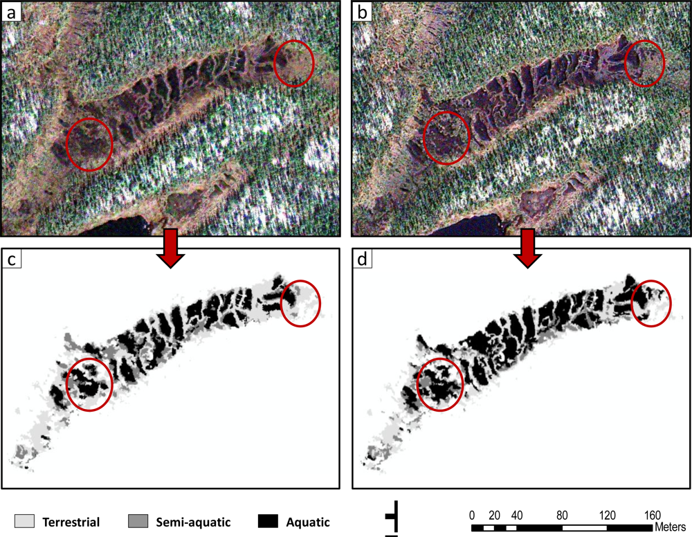
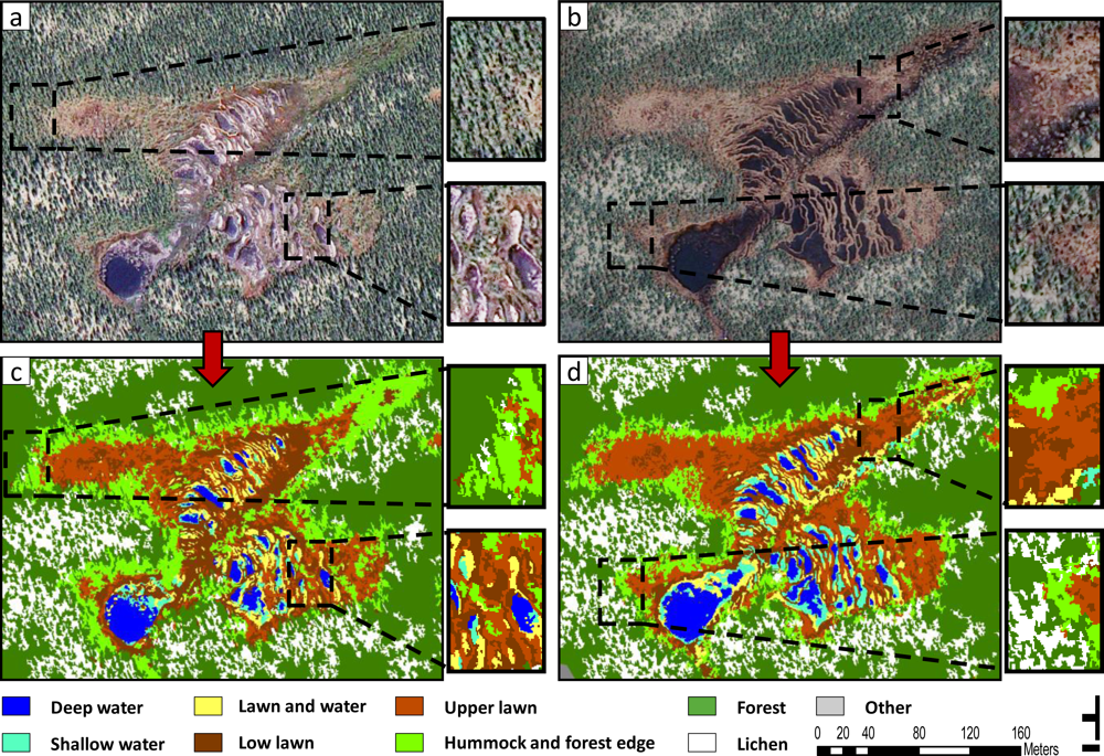
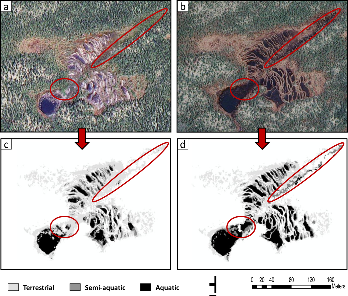
Two GeoEye-1 image subsets centered on site 1 are shown in Figure 5 with their respective fine-scale classifications. These subsets were chosen because the hydrological conditions (in particular, the discharge values) they recorded, differed greatly. The white and grey zones in the 23 July 2009 image were caused by sunglint, which separated the “shallow water” and the “lawn and water” from the other environments (Figure 5(a,c)). Visual correspondence between the two classifications and the two RGB images was very good. Most of the errors appeared on the border of the site 1 fen (caused by non-restrictive rule sets applied to the “transition” class), where they had no effect on the results of the hydrological study (Figure 5(a–d)). Misclassifications appeared also on the 18 May 2010 image due to the phenological stage of shrub vegetation. Many hummocks were classified as “upper lawn” or “low lawn”, (Figure 5(b,d)) since shrubs on these hummocks were not green at this season and discriminant features were based on greenness indices.
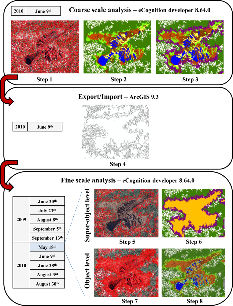
Classification accuracy was assessed using the confusion matrix method. The classification accuracy results of the 9 June 2010 image (coarse scale: Step 2), used as the reference image, are given in Table 3 and Table 4. The confusion matrix in Table 3 shows the accuracy results of the original classes, while the matrix in Table 4 shows the accuracy results of environmental groupings (Table 2) of the original classes. The overall accuracy of the original classes was 86% and the Kappa coefficient was 84% (Table 3). The majority of misclassifications appearing in this first matrix were not relevant. The confusion matrix based on environmental groupings gave better results, showing an overall accuracy of 93% and a Kappa coefficient of 90%. This ensured high accuracies for the subsequent fine classifications of all 10 images, avoiding most of the error propagation due to class-related hierarchical features. The most important issue was confusion between objects in the FOREST group and objects in the PEAT group (32 out of 554 objects in these groups). To manage this imperfect delineation of peatlands, a “transition” class was created (coarse scale: Step 3) after the first classification of the 9 June 2010 image. The transition area was then reclassified at a finer scale (Step 8) as either forest or peatland.
The fine-scale classification accuracy results of the 10 images (Step 8) are given in Tables 5 and 6. Table 5 shows the accuracy results of the original classes. Table 6 shows those of hydrological groupings of the original classes. The groupings were functions of the saturation degree (aquatic, semi-aquatic, terrestrial) of the classes. These groupings were very helpful for monitoring the seasonal spatial dynamics of the hydrology at the study sites. The “open water” and “shallow water” classes were included in the AQUATIC group, the “lawn and water” class was included in the SEMI-AQUATIC group, and the remaining classes were included in the TERRESTRIAL group.
The classifications of the original classes had an overall accuracy of 82% and a kappa coefficient of 79% (Table 5). This high level of accuracy indicates the robustness of the specific object-based rulesets developed in order to investigate the hydrological dynamics at an intra-seasonal scale with multispectral imagery. The “open water”, “upper lawn”, and “lichen” classes were well-classified since their spectral features were easily distinguishable. However, some significant confusion can be observed between the other classes. The producer’s accuracies of the “forest” and “hummock and forest edge” classes were under 70%. Moreover, the user’s accuracies of the “shallow water”, “lawn and water”, and “low lawn” classes were under 75%. Since the transition area between peatland and forest was reclassified at a fine scale, it was considered in the confusion matrices. This transition area is a highly heterogeneous environment (containing peat, shrubs, trees, and their shadows) with non-restrictive applied rulesets. Thus, very small objects were generated, which sometimes caused classification problems. For example, objects corresponding to tree shadows were easily misclassified as “shallow water” since they were spectrally homogeneous and dark.
The accuracy results of the hydrological groupings were higher, with an overall accuracy of 92% and a kappa coefficient of 83% (Table 6). The accuracy of the SEMI-AQUATIC group was lower than those of the AQUATIC and TERRESTRIAL groups. This can be explained by the nature of the SEMI-AQUATIC group, which was created from a single class and represents a transitory environment. The producer’s accuracies of the AQUATIC and SEMI-AQUATIC groups were 97% and 84%, respectively. These results indicate a low level of omission error, which means that the majority of the aquatic and semi-aquatic compartments of the peatlands were detected effectively in the satellite images. Such accuracies were necessary in order to study the spatial dynamics of these compartments (see Section 3.2). The user’s accuracies of the AQUATIC and SEMI-AQUATIC groups were 87% and 64%, respectively. These results indicate a higher level of commission error, leading to overestimation of the area of the aquatic and semi-aquatic compartments. A significant number of TERRESTRIAL objects were misclassified as SEMI-AQUATIC (216 objects) or AQUATIC objects (116 objects). These TERRESTRIAL objects were most often “forest” or “hummock and forest edge” objects (Table 5). The overestimation of the area of the aquatic and semi-aquatic compartments was not critical for our further study of the spatial dynamics of these compartments. Indeed, the heterogeneous environment of the transition area, where most of the confusion appeared, remains outside the limits of the later defined saturation area (see Section 3.2).

3.2. Seasonal Spatial Dynamics of Aquatic and Semi-Aquatic Structures in Fens

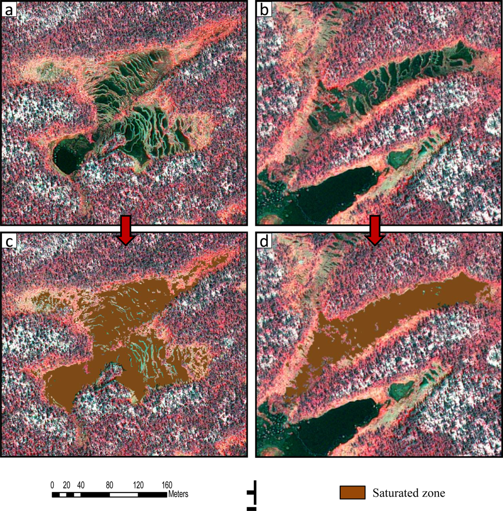
In order to study the evolution of the hydrology of the peatlands, the saturated zone was delineated for both peatlands. This zone includes the terrestrial, semi-aquatic, and aquatic compartments, which are spatially dynamic. The saturated zone is affected by the presence of water at or near the surface (<10 cm deep), which influences the composition of its vegetation cover [40]. The following classes were considered as saturated: “low lawn”, “lawn and water”, “shallow water”, and “deep water”. The 3 August 2010 classification map was chosen to delineate the saturated zone in both fens under study. This map was chosen because green vegetation (high contrast with saturated peat) and wet conditions enabled precise delineation of the saturated zone (Figure 6).
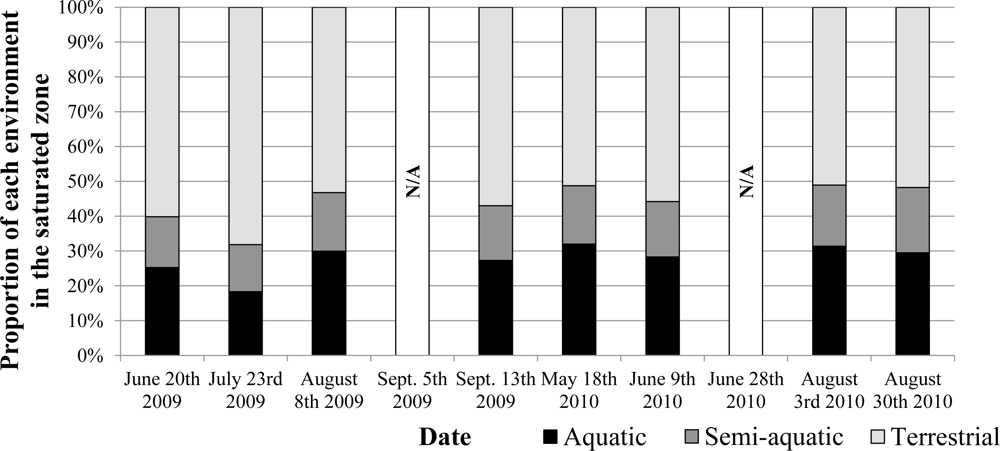
Within the site 1 saturated zone, the aquatic (“open water” and “shallow water” classes), semi-aquatic (“lawn and water” class), and terrestrial proportions were calculated from the 10 image classifications; these proportions are shown in Figure 7. The results demonstrate the existence of significant seasonal spatial dynamics of the compartments. The aquatic proportion of the saturated zone varied between 18% at the driest conditions observed (23 July 2009: no precipitation, snowmelt ended, high evapotranspiration rate) and 32% at the wettest period observed (18 May 2010: snowmelt, low evapotranspiration rate), corresponding to an increase of 78%. The increase in the combined aquatic and semi-aquatic proportions of the saturated zone was 53% (from 32% to 49%). As shown in Figure 8 (encircled features), between the driest and the wettest conditions observed, strong spatial dynamics occurred upstream of the largest pool at the outlet of the site 1 fen. The north-eastern part of the fen (upstream) was also subject to significant spatial dynamics, with temporary pools appearing on the 18 May 2010 image.
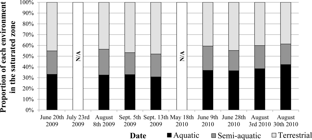
Within the site 2 saturated zone, significant seasonal spatial dynamics of the compartments was also noticed (Figure 9), but of smaller magnitude. Unfortunately, there were clouds over site 2 on 23 July 2009 and 18 May 2010, the respective dates on which the driest and the wettest conditions were observed at site 1. Thus, the amplitude of the seasonal spatial dynamics cannot be directly compared between the two sites. The aquatic proportion of the site 2 saturated zone varied between 31% at the driest conditions observed (13 September 2009: no precipitation, snowmelt ended) and 42% at the wettest period observed (30 August 2010: precipitation, low evapotranspiration rate), corresponding to an increase of 35%. The increase in the combined aquatic and semi-aquatic proportions of the saturated zone was 17% (from 52% to 61%). As shown in Figure 10 (encircled features), between the driest and the wettest conditions observed, strong spatial dynamics occurred on the edges of some of the main pools. The eastern part of the fen (downstream) was also subject to significant spatial dynamics, with temporary pools appearing on the 30 August 2010 image.

3.3. Seasonal Spatial Dynamics in Relation to the Hydrological Regime of Fens

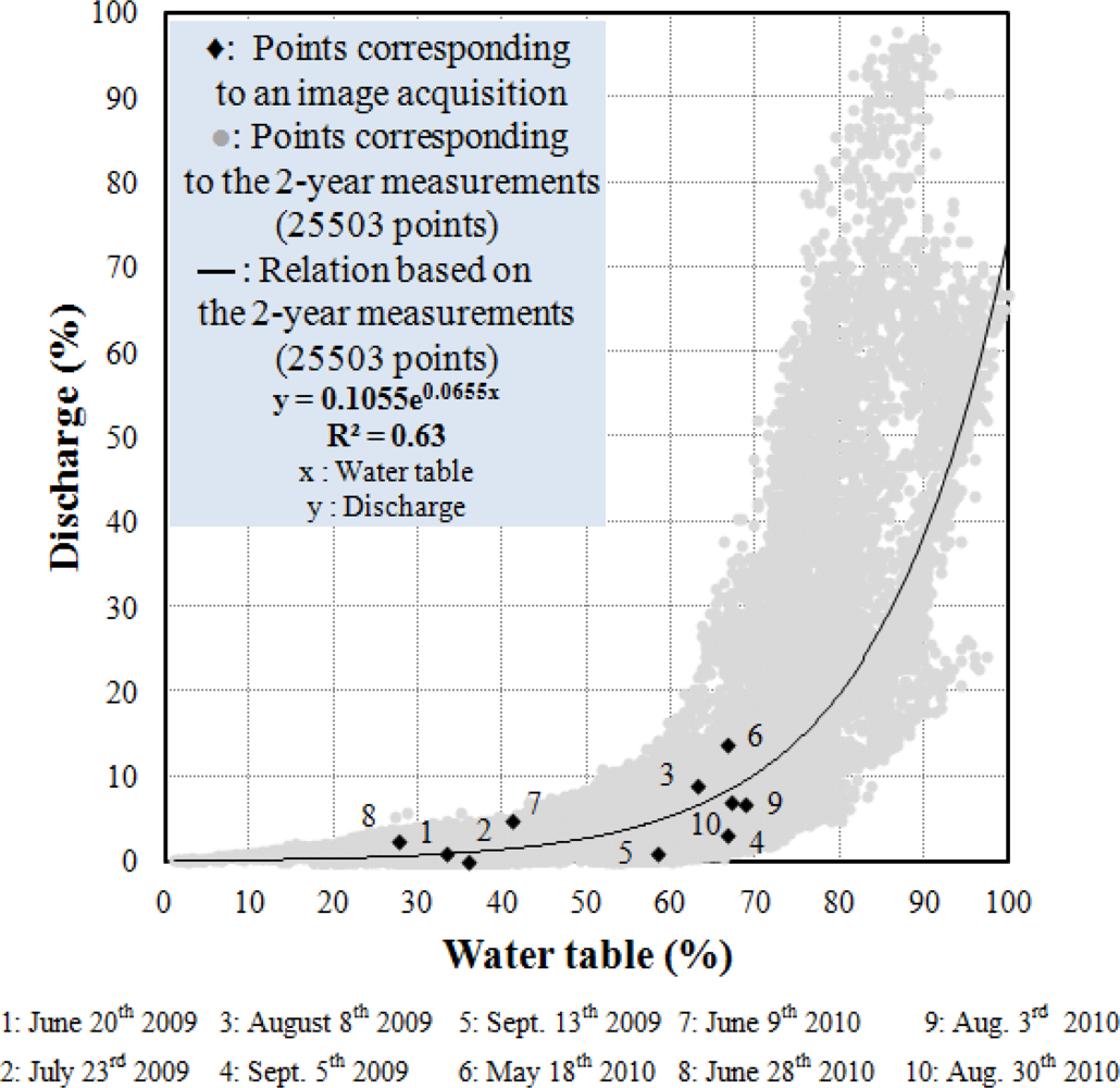
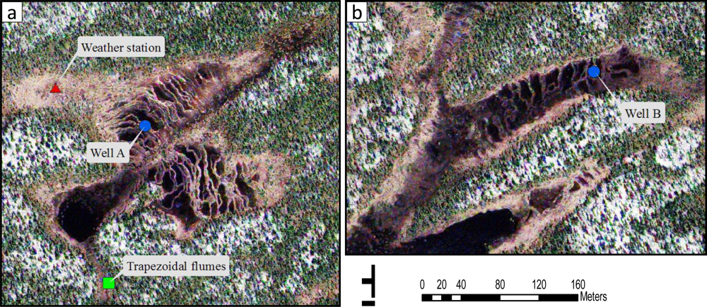
Figure 11 shows the relationship between the water table level measured at well A and the discharge measured at the outlet of the site 1 fen. The water table data is of course derived from a local measurement, whereas discharge measure is the consequence of runoff in the whole fen watershed. We assumed, however, that water table changes were relatively homogeneous throughout each site. On Figure 11, each point corresponds to a pair of water table and discharge measurements taken at 15-min intervals during the 2009 and 2010 snow-free seasons. The range of measured values is displayed in percentages to facilitate comparison with subsequent graphs. These percentages were calculated relative to the maximal water table and discharge values during the two-year period.
An exponential relation was found between water table and discharge values, similar to the one reported in previous hydrological studies on patterned peatlands [9,11,47], with a coefficient of determination of 0.63. Two phases can be distinguished in the evolution of discharge values relative to the water table. In the first phase, the water table rises rapidly but discharge remains low. For example, the water level may equal 60% of the maximal measured water level while the corresponding discharge is equal to only 5% of the maximal measured discharge. In this phase, the incoming water contributes to an increase in the water level in the fen but not to a significant evolution of the discharge: it is a storage phase. In the second phase, the water level is already high and does not increase much but there is a sharp increase in discharge from the fen: this phase is a runoff phase. For the purposes of modeling this regime, it is particularly important to identify the threshold on the relation where the regime phase changes. Since heavy rainfall can lead to heavy runoff in one phase and no runoff in the other phase, successful modeling of hydrological behavior in fens hinges on distinction of the two phases [47]. However, water table values often vary as much as 30% for a given value of discharge. This high dispersion of water table values may be explained by a hysteresis effect [11,48]. Depending on whether the runoff significantly increases or significantly decreases, the relation between water table and discharge reacts slightly differently. This creates some uncertainties for modeling of the regime phases and thus needs to be considered.
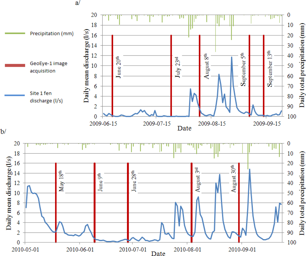
In situ hydrometric measurements taken at the same time as the satellite images used in this project are highlighted in Figure 11. The GeoEye-1 images were acquired during varying hydrological conditions, at the beginning and the end of the storage phase. Among the acquired images, the driest hydrological conditions (corresponding to the beginning of the storage phase) occurred on 20 June 2009, 23 July 2009, 28 June 2010, and 9 June 2010. The dry hydrological conditions on these dates resulted from the long duration of the day and high temperatures experienced during the months of June and July [28]. These conditions imply a higher evapotranspiration rate in peatlands. By this time of year, the snowmelt had also ended. The remaining 6 images were acquired during wetter hydrological conditions corresponding to the end of the storage phase. These images were acquired in May, August, and September 2009 and 2010. In May, the snowmelt often produces wet hydrological conditions in peatlands [49]. In August and September, the days shorten and mean temperature falls [28], causing a relatively low evapotranspiration rate [40]. Unfortunately, for reasons explained in Section 2.3.1 no image was acquired during the runoff phase. Nevertheless, as seen in Section 3.2, our satellite image classifications showed that the seasonal spatial dynamics of aquatic and semi-aquatic structures in the fens was substantial. The lack of images of high discharge events was not an obstacle to observation of the seasonal hydrological dynamics. These dynamics were considerable during the storage phase and seemed to be related to the evolution of the water level.
In the following analysis, links between the evolution of the measured water levels and the spatial dynamics of the aquatic and semi-aquatic compartments were assessed. The aquatic compartments of the saturated zone could have been chosen as the only indicators of the spatial dynamics of the hydrology of the sites. We chose to include the semi-aquatic compartments as well, as they play an integral part in these dynamics. We must remain cautious about this inclusion, however, since the results of the last confusion matrix (Table 6) showed that the SEMI-AQUATIC group was less precisely classified than the other groups.
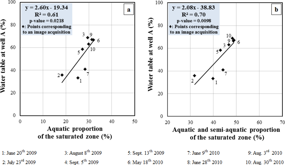
Figure 12 shows the water table variation measured in site 1 compared to the spatial variation of the aquatic and semi-aquatic compartments within site 1 (derived from eight GeoEye-1 classifications). Linear correlations were established in all cases. Over 60% of the water table variation was explained by the spatial variation of the aquatic and semi-aquatic compartments. These correlations were significant with a p-value < 0.05. The slope of the linear functions was always positive. This implies that higher “aquatic” and “aquatic and semi-aquatic” proportions of the saturated zone indicate a higher water table. This result enabled us to validate once more the precision of the performed classifications and their relevance for tracking real hydrological variations.
However, as noted above, the water table data are derived from a local measurement (a single point), while the classification-derived results describe the whole saturated zone of the fen. The dynamics of the water table can vary at different locations in a single fen. This may explain why the points differ so much from the linear model on some dates (20 June 2009, 9 June 2010).
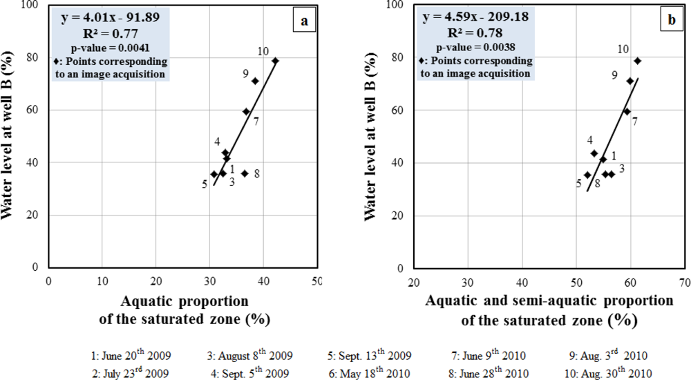
Figure 13 shows the water level variation measured in site 2 compared to the spatial variation of the aquatic and semi-aquatic compartments within site 2 (derived from eight GeoEye-1 classifications). Linear correlations were established in all cases. Over 75% of the water level variation was explained by the spatial variation of the aquatic and semi-aquatic compartments. These correlations were significant with a p-value < 0.05. The slope of the linear functions was always positive. As for the site 1 fen, this relation implies that higher “aquatic” and “aquatic and semi-aquatic” proportions of the saturated zone indicate a higher water level. This result also enabled us to validate the precision of the performed classifications and their relevance for tracking real hydrological variations.
There was a significant difference between the R2 values of the water levels measured in well A and those measured in well B. R2 was always lower in the first case than in the second case. This difference may be explained by the different types of measurements made. Groundwater level (under the lawn surface) was measured at well A, whereas open water level (at the pool surface) was measured at well B. The statistics derived from the classifications were related to hydrological variations at the surface of the fen and should therefore be better correlated with the evolution of pool water levels than with that of groundwater levels.
The slopes of the linear relations in Figure 13 (site 2 fen) are around two times steeper than those in Figure 12 (site 1 fen), reflecting weaker spatial dynamics of the aquatic and semi-aquatic compartments in the site 2 fen. The internal structures of the fens undoubtedly influence these slopes. Morphological features such as pool area, pool depth, and pool outlines provide some indication of the structure of the peatland [50]. We hypothesize that well-defined pool outlines indicate insignificant spatial dynamics in the aquatic and semi-aquatic compartments. Loose outlines, on the other hand, suggest major spatial dynamics in the aquatic and semi-aquatic compartments. In the latter case, the incoming water cannot be stored vertically in the pool, so it spreads horizontally, which explains why the aquatic and semi-aquatic spatial dynamics appear in the imagery. To assess this hypothesis, a comparison between the pools of the two sites was made. The pools are generally large on site 2 (Figure 10), whereas the proportion of large and small pools is more balanced on site 1 (Figure 8). White found a positive correlation between pool area and pool depth [50]. The same study also found that pools with a sharp contour were significantly larger than those with a loose outline [50]. Overall, small pools tended to be shallow and to have a loose outline, while large pools tended to be deep and to have a sharp outline. Our hypothesis suggests that these characteristics should lead to stronger aquatic and semi-aquatic spatial dynamics at site 1 than at site 2. However, the strong dynamics observed at site 1 were caused by more than just the presence of small pools with loose outlines. As noted above, a very large pool near the outlet of the site 1 fen also made major contributions (Figure 8). Water tends to be stored downslope in the fen [50]. Large amounts of water coming irregularly from the two wings of the fen induced the strong spatial dynamics upstream of the pool. To better understand the degree to which various morphological parameters (pool area, depth, outlines) influence the magnitude of increases in the proportion of aquatic and semi-aquatic compartments, more sites with very different morphological features should be monitored in the future.

4. Conclusions

The aim of this work was to investigate the seasonal hydrological dynamics of minerotrophic peatlands (fens) with the help of multi-date GeoEye-1 VHR imagery. This was done in order to answer the following questions: “Is it possible to delineate and classify the internal structures of peatlands with the help of VHR multispectral images?”; “Are there seasonal dynamics of aquatic and semi-aquatic structures in patterned fens and can this be quantified with these images?”; and “Can the observed dynamics be linked with the hydrological regime of fens?”.
For these purposes, an object-based classification approach was set up and applied to 10 GeoEye-1 images acquired during the snow-free seasons of 2009 and 2010 over two fens (site 1 and 2) located in the La Grande river basin (54°N, Quebec, Canada). In addition, continuous hydrometeorological monitoring was instigated in 2009 of these fens.
The object-based classification approach provided a satisfactory level of accuracy both for the delineation of peatlands (overall accuracy of 93%) and for the distinction of the internal structures of peatlands (overall accuracy of 82%). Spectral quality and spatial resolution of GeoEye-1 fused imagery was sufficient to discriminate the ecohydrological features in a complex peatlands environment. The multispectral data has been particularly important in separating aquatic, semi-aquatic and terrestrial classes. Indeed, the vegetation presence and the saturation degree greatly influenced the spectral response of these bands.
Moreover, the time series of the internal peatlands structures mapping demonstrated the existence of important intraseasonal spatial dynamics in the aquatic and semi-aquatic compartments of the peatlands under study (site 1: 53% of variation; site 2: 17% of variation). It was revealed that the dynamics amplitude depended on the morphological features of the fens. The spatial dynamics appear stronger if pool outlines are indistinct than when they are well-defined. Even if the 10 images were acquired during low-flow conditions, almost all of the intraseasonal dynamics of the aquatic and semi-aquatic compartments were captured by the imagery.
The observed spatial dynamics were closely related to the evolution of the measured water levels. Indeed, when analyzing the relationship between peatland water level and discharge, two distinct hydrological regimes were observed. The first is the storage phase during which a high increase of the peatland water level does not result in significant increase of the outlet discharge. During this phase, the spatial extent of the aquatic and semi-aquatic compartments, extracted from the imagery, greatly increases. From a certain threshold, there is high increase of the discharge which does not result in significant increase of the water level. During this runoff phase, spatial extent of aquatic and semi-aquatic compartments should not increase significantly. Thus, establishing the threshold of regime change by satellite imagery would allow determining the storage capacity of a fen. This is of great importance for understanding and modeling the hydrology of patterned peatlands. This study has demonstrated the possibility of a hydrological monitoring of peatlands at both intraseasonal and local scale. Previous studies were limited to hydrological monitoring at multi-decadal scale.
This work was conducted over only two experimental sites. It would be interesting to repeat the experience on other peatlands with a morphological gradient. This would enable quantifying the storage capacity and detecting the position of the threshold of hydrological regime change, from the spatial variations of aquatic and semi-aquatic structures extracted from VHR multispectral imagery. In this case, care should be taken to measure the flow at the outlet of each fen (in the present study, only one fen outlet was instrumented). In addition, water table measurements should be located in strategic areas where spatial hydrological dynamics is important, for example in pools with indistinct outlines. Sites could be adequately identified and selected using imagery. This study is the primordial stage in the development of operational approaches of hydrological monitoring in patterned fens using VHR multispectral imagery. The synoptic view complements, or, offers even an alternative to, peatland field instrumentation, especially in remote areas.

Acknowledgments

This research was funded by the Natural Sciences and Engineering Research Council of Canada (NSERC) and Hydro-Quebec as part of the project “Ecohydrology in highly aqualysed fens of La Grande River watershed”. The authors would like to gratefully acknowledge them for their financial support. The authors wish also to thank G. Carrer, S. Proulx-McInnis, N. Cliche Trudeau, G. Levrel, M. White, M. Dissanska, A. Jacome, J. Poulin, and Y. Gauthier for their assistance. Finally, the authors are grateful for the hydrological data provided by the INRS hydrology team.

References

  1. Hydro-Québec Complexe Hydroélectrique la Grande. Available online: http://www.hydroquebec.com/developpementdurable/documentation/pdf/poissons/fiche_12.pdf (accessed on 12 August 2011).
  2. Faune, M.R.N. La Stratégie Énergétique du Québec 2006–2015. 2006. Available online: http://www.mrnf.gouv.qc.ca/publications/energie/strategie/strategie-energetique-2006-2015.pdf (accessed on 13 September 2011).
  3. Roy, R. S’Adapter aux Changements Climatiques: La Production d’Hydroélectricité. Available online: http://www.ouranos.ca/fr/pdf/ouranos_sadapterauxcc_fr.pdf (accessed on 5 October 2011).
  4. National Wetlands Working Group, The Canadian Wetlands Classification System, 2nd ed; Warner, B.G.; Rubec, C.D.A. (Eds.) Wetlands Research Centre, University of Waterloo: Waterloo, ON, Canada, 1997; p. 68.
  5. Waddington, J.M.; Quinton, W.L.; Price, J.S.; Lafleur, P.M. Advances in Canadian peatland hydrology, 2003–2007. Can. Water Resour. J 2009, 34, 139–148. [Google Scholar]
  6. Tarnocai, C.; Kettles, I.M.; Lacelle, B. Peatlands of Canada Map; Scale 1: 6 500 000; Open File 3834; Geological Survey of Canada: Ottawa, ON, Canada, 2000. [Google Scholar]
  7. Price, J.S.; Maloney, D.A.; Downey, F.G. Peatlands of the Lake Melville Coastal Plain, Labrador. Northern Hydrology: Selected Perspectives: Proceedings of the Northern Hydrology Symposium, Saskatoon, Saskatchewan, 10–12 July 1990; Northern Hydrology: Saskatoon, SK, Canada, 1990; pp. 293–302. [Google Scholar]
  8. Price, J.S.; Maloney, D.A. Hydrology of a Patterned Bog-Fen Complex in Southeastern Labrador, Canada; Nordic Association for Hydrology: Lyngby, Danemark, 1994; Volume 25. [Google Scholar]
  9. Quinton, W.L.; Roulet, N.T. Spring and summer runoff hydrology of a subarctic patterned wetland. Arctic Alpine Res 1998, 30, 285–294. [Google Scholar]
  10. Price, J.S.; Waddington, J.M. Advances in canadian wetland hydrology an biogeochemistry. Hydrol. Process 2000, 14, 1579–1589. [Google Scholar]
  11. Clerc, C. Suivi de la Nappe, de la Recharge et de l’Écoulement à l’Aide de Méthodes in situ afin de Comprendre la Dynamique de Tourbières Ombrotrophes de la Région de la Baie de James; Mémoire de Maîtrise En Sciences de l’Eau, INRS-ÉTÉ: Québec City, QC, Canada, 2009. [Google Scholar]
  12. Tardif, S.; St-Hilaire, A.; Roy, R.; Bernier, M.; Payette, S. Statistical properties of hydrographs in minerotrophic fens and small lakes in mid-latitude quebec, canada. Can. Water Resour. J 2009, 34, 365–379. [Google Scholar]
  13. Ozesmi, S.L.; Bauer, M.E. Satellite remote sensing of wetlands. Wetl. Ecol. Manag 2002, 10, 381–402. [Google Scholar]
  14. Rokitnicki-Wojcik, D.; Wei, A.H.; Chow-Fraser, P. Transferability of object-based rule sets for mapping coastal high marsh habitat among different regions in georgian bay, canada. Wetl. Ecol. Manag 2011, 19, 223–236. [Google Scholar]
  15. Ghedira, H. Utilisation des Réseaux de Neurones pour la Cartographie des Milieux Humides à Partir d’une Série Temporelle d’Images Radarsat-1. Ph.D. Thesis, INRS-ETE, Quebec City, QC, Canada. 2002. [Google Scholar]
  16. Bernier, M.; Ghedira, H.; Gauthier, Y.; Magagi, R.; Filion, R.; De Seve, D.; Ouarda, T.; Villeneuve, J.P.; Buteau, P. Remote sensing and classification bogs in quebec using radarsat-1 images. Can. J. Remote Sens 2003, 29, 88–98. [Google Scholar]
  17. Grenier, M.; Demers, A.M.; Labrecque, S.; Benoit, M.; Fournier, R.A.; Drolet, B. An object-based method to map wetland using radarsat-1 and landsat etm images: Test case on two sites in quebec, canada. Can. J. Remote Sens 2007, 33, S28–S45. [Google Scholar]
  18. Quinton, W.L.; Hayashi, M.; Pietroniro, A. Connectivity and storage functions of channel fens and flat bogs in northern basins. Hydrol. Process 2003, 17, 3665–3684. [Google Scholar]
  19. Racine, M.J.; Bernier, M.; Ouarda, T. Evaluation of radarsat-1 images acquired in fine mode for the study of boreal peatlands: A case study in james bay, canada. Can. J. Remote Sens 2005, 31, 450–467. [Google Scholar]
  20. Töyrä, J.; Pietroniro, A. Towards operational monitoring of a northern wetland using geomatics-based techniques. Remote Sens. Environ 2005, 97, 174–191. [Google Scholar]
  21. Dissanska, M.; Bernier, M.; Rousseau, A.N.; Chokmani, K.; Jutras, S. Étude de la Connectivité Physique des Tourbières au Réseau Hydrographique du Bassin versant de la Grande Rivière à l’Aide d’une Classification Orientée Objet d’Images Landsat-7 ETM+: Rapport de Recherche; R927; INRS-ETE: Quebec, QC, Canada, 2007; pp. 1–63. [Google Scholar]
  22. Gómez-Rodríguez, C.; Bustamante, J.; Díaz-Paniagua, C. Evidence of hydroperiod shortening in a preserved system of temporary ponds. Remote Sens 2010, 2, 1439–1462. [Google Scholar]
  23. Collins, M. Caractérisation des Tourbières et Suivi Historique des Unités Morphologiques de Surface en lien avec le Climat dans le Bassin versant de la Rivière la Grande au Québec. M.Sc. Thesis, Université du Québec à Montréal, Montréal, QC, Canada. 2005. [Google Scholar]
  24. Novack, T.; Esch, T.; Kux, H.; Stilla, U. Machine learning comparison between worldview-2 and quickbird-2-simulated imagery regarding object-based urban land cover classification. Remote Sens 2011, 3, 2263–2282. [Google Scholar]
  25. Moskal, L.M.; Styers, D.M.; Halabisky, M. Monitoring urban tree cover using object-based image analysis and public domain remotely sensed data. Remote Sens 2011, 3, 2243–2262. [Google Scholar]
  26. Dissanska, M.; Bernier, M.; Payette, S. Object-based classification of very high resolution panchromatic images for evaluating recent change in the structure of patterned peatlands. Can. J. Remote Sens 2009, 35, 189–215. [Google Scholar]
  27. Soti, V.; Puech, C.; Lo Seen, D.; Bertran, A.; Vignolles, C.; Mondet, B.; Dessay, N.; Tran, A. The potential for remote sensing and hydrologic modelling to assess the spatio-temporal dynamics of ponds in the ferlo region (senegal). Hydrol. Earth System Sci 2010, 14, 1449–1464. [Google Scholar]
  28. Bootsma, A.; Ballard, M. A National Ecological Framework for Canada. Appendix 1: Canadian Ecodistrict Climate Normals 1961–1990 Overview. 1997. Available online: http://sis.agr.gc.ca/cansis/nsdb/ecostrat/district/climate.html (accessed on 10 October 2011).
  29. Proulx-McInnis, S. Caractérisations Hydrologique, Topographique et Géomorphologique d’un Bassin versant Incluant une Tourbière Minérotrophe Fortement Aqualysée, baie-de-james, Québec. M.Sc. Thesis, INRS-ETE, Québec City, QC, Canada. 2010. [Google Scholar]
  30. Schowegerdt, R.A. Remote Sensing: Models and Methods for Image Processing, 2nd ed; Academic Press: San Diego, CA,USA, 1997. [Google Scholar]
  31. Krause, K. Radiometric Use of Quickbird Imagery; DigitalGlobe: Longmont, CO, USA, 2005. Available online: http://www.digitalglobe.com/downloads/QuickBird_technote_raduse_v1.pdf (accessed on 12 August 2011).
  32. Zhang, Y. A New Automatic Approach for Effectively Fusing Landsat-7 as well as IKONOS Images. Proceedings of IEEE International Geosciences and Remote Sensing Symposium, Toronto, ON, Canada, 24–28 June 2002; pp. 2429–2243.
  33. Nikolakopoulos, K.G. Pansharp vs. wavelet vs PCA fusion technique for use with Landsat ETM panchromatic and multispectral data. Proc. SPIE 2004. [Google Scholar] [CrossRef]
  34. Jensen, J.R. Remote Sensing Atmospheric Correction. In Introductory Digital Image Processing: A Remote Sensing Perspective, 3rd ed; Chapter 6; Prentice-Hall: Englewood Cliffs, NJ, USA, 2005; pp. 175–225. [Google Scholar]
  35. Blaschke, T.; Lang, S.; Hay, G.J. Geographic Object-Based Image Analysis (GEOBIA): A New Name for a New Discipline. In Object-Based Image Analysis. Spatial Concepts for Knowledge-Driven Remote Sensing Applications; Chapter 1.4; Springer-Verlag: Berlin, Germany; p. 2008.
  36. Grenier, M.; Labrecque, S.; Garneau, M.; Tremblay, A. Object-based classification of a SPOT-4 image for mapping wetlands in the context of greenhouse gases emissions: The case of the eastmain region, Québec, Canada. Can. J. Remote Sens 2008, 34, S398–S413. [Google Scholar]
  37. Benz, U.C.; Hoffman, P.; Willhauck, G.; Lingenfelder, I.; Heynen, M. Multi-resolution, object-oriented fuzzy analysis of remote sensing data for GIS-ready information. ISPRS J. Photogramm 2004, 58, 239–258. [Google Scholar]
  38. Trimble, Ecognition 8.64.0 User Guide; Trimble GmbH: Munich, Germany, 2010; pp. 1–250.
  39. Levrel, G.; Rousseau, A.N. Étalonnage des Sondes FDR (Frequency Domain Reflectometry) sur les Cinq Premiers Centimètres des sols et des Couverts de Bryophytes de deux Tourbières du Milieu Boréal Québécois; INRS-ETE: Québec City, QC, Canada, 2010; pp. 1–315. [Google Scholar]
  40. Payette, S.; Rochefort, L. Écologie des Tourbières du Québec-Labrador; Presses Université Laval: Québec City, QC, Canada, 2001. [Google Scholar]
  41. Waddington, J.M.; Kellner, E.; Strack, M.; Price, J.S. Differential peat deformation, compressibility, and water storage between peatland microforms: Implications for ecosystem function and development. Water Resour. Res 2010, 46, W07538. [Google Scholar]
  42. Mitrakis, N.E.; Topaloglou, C.A.; Alexandridis, T.K.; Theocharis, J.B.; Zalidis, G.C. A novel self-organizing neuro-fuzzy multilayered classifier for land cover classification of a vhr image. Int. J. Remote Sens 2008, 29, 4061–4087. [Google Scholar]
  43. Harris, A.; Bryant, R.G. A multi-scale remote sensing approach for monitoring northern peatland hydrology: Present possibilities and future challenges. J. Environ. Manage 2009, 90, 2178–2188. [Google Scholar]
  44. Tuxen, K.A.; Schile, L.M.; Kelly, M.; Siegel, S.W. Vegetation colonization in a restoring tidal marsh: A remote sensing approach. Restor. Ecol 2008, 16, 313–323. [Google Scholar]
  45. Barrette, J.; August, P.; Golet, F. Accuracy assessment of wetland boundary delineation using aerial photography and digital orthophotography. Photogramm. Eng. Remote Sensing 2000, 66, 409–416. [Google Scholar]
  46. Congalton, R.G.; Green, K. Assessing the Accuracy of Remotely Sensed Data: Principles and Practices; CRC Press: Boca Raton, FL, USA, 1999. [Google Scholar]
  47. Jutras, S.; Rousseau, A.N.; Clerc, C.M. Implementation of a peatland-specific water budget algorithm in hydrotel. Can. Water Resour. J 2009, 34, 349–364. [Google Scholar]
  48. Weiss, R.; Shurpali, N.J.; Sallantaus, T.; Laiho, R.; Laine, J.; Alm, J. Simulation of water table level and peat temperatures in boreal peatlands. Ecol. Model 2006, 192, 441–456. [Google Scholar]
  49. Glenn, M.; Woo, M.-K. Spring and summer hydrology of a valley-bottom wetland, ellesmere island, northwest territories, canada. Wetlands 1997, 17, 321–329. [Google Scholar]
  50. White, M. Modèle de Développement des Tourbières Minérotrophes Aqualysées du Haut-Boréal Québécois. M.Sc. Thesis, Université Laval, Quebec City, QC, Canada. 2011. [Google Scholar]
Figure 1. Location map of the two study site watersheds in the James Bay region, Quebec, Canada.
Remotesensing 04 01887f1
Figure 2. Location of the instruments used in the study at (a) site 1 (54°06′52″N, 72°30′02″W) and (b) site 2 (54°06′41″N, 72°30′56″W).
Remotesensing 04 01887f2
Figure 3. GeoEye-1 image acquisitions and hydrological conditions during: (a) spring and summer 2009; (b) spring and summer 2010.
Remotesensing 04 01887f3
Figure 4. Scheme of the object-based analysis procedure.
Remotesensing 04 01887f4
Figure 5. Comparison between (a) 23 July 2009 and (b) 18 May 2010 RGB images (subsets centered on site 1: 54°06′52″N, 72°30′02″W), and their respective fine-scale classifications (Step 8) (c,d). Areas of sunglint and of major misclassifications are expanded.
Remotesensing 04 01887f5
Figure 6. False colored composite (NIR, Red, Green) of two 3 August 2010 GeoEye-1 subsets centered on (a) site 1 (54°06′52″N, 72°30′02″W) and (b) site 2 (54°06′41″N, 72°30′56″W). The locations of the respective saturated zones of each fen appear in (c,d).
Remotesensing 04 01887f6
Figure 7. Aquatic, semi-aquatic, and terrestrial proportions of the site 1 saturated zone for each GeoEye-1 image acquisition date. The term N/A refers to missing data due to the presence of clouds over site 1.
Remotesensing 04 01887f7
Figure 8. Comparison between (a) 23 July 2009 and (b) 18 May 2010 GeoEye-1 RGB images (subsets centered on site 1: 54°06′52″N, 72°30′02″W), and the respective aquatic, semi-aquatic, and terrestrial proportions of the site 1 saturated zone (c,d). Areas of major change are encircled in red.
Remotesensing 04 01887f8
Figure 9. Aquatic, semi-aquatic, and terrestrial proportions of the site 2 saturated zone for each GeoEye-1 image acquisition date. The term N/A refers to missing data due to the presence of clouds over site 2.
Remotesensing 04 01887f9
Figure 10. Comparison between (a) 13 September 2009 and (b) 30 August 2010 GeoEye-1 RGB images (subsets centered on site 2: 54°06′41″N, 72°30′56″W), and the respective aquatic, semi-aquatic, and terrestrial proportions of the site 2 saturated zone (c,d). Areas of major change are encircled in red.
Remotesensing 04 01887f10
Figure 11. Discharge of the site 1 fen is related to the water table measured at well A. Discharge and water table data were collected every 15 minutes during the 2009 and 2010 snow-free seasons. The range of measured values is displayed in percentages, 100% corresponding to the maximal measured value (0% to the minimal). Black diamonds show discharge and water table values corresponding to image acquisitions.
Remotesensing 04 01887f11
Figure 12. (a) Water table measured at well A compared to corresponding aquatic proportion of the site 1 saturated zone (derived from GeoEye-1 image classifications). (b) Water table measured at well A compared to corresponding aquatic and semi-aquatic proportion of the site 1 saturated zone. The range of measured water table values is displayed in percentages, 100% corresponding to the maximal water table value (0% to the minimal).
Remotesensing 04 01887f12
Figure 13. (a) Water level measured at well B compared to corresponding aquatic proportion of the site 2 saturated zone (derived from GeoEye-1 image classifications). (b) Water level measured at well B compared to corresponding aquatic and semi-aquatic proportion of the site 2 saturated zone. The range of measured water levels is displayed in percentages, 100% corresponding to the maximal water level value (0% to the minimal).
Remotesensing 04 01887f13
Table 1. Features of the acquired GeoEye-1 images.
GeoEye-1 Images Features2009
2010
Jun 20Jul 23Aug 8Sep 5Sep 13May 18Jun 9Jun 28Aug 3Aug 30
Ground coverage (km)7.9 × 7.77.9 × 7.77.9 × 7.77.9 × 7.77.9 × 7.77.9 × 7.78.0 × 8.07.9 × 7.77.9 × 7.78.0 × 8.0
Sensor tilt (°)16.6928.427.9525.6714.8727.5415.5110.3726.9317.94
Nominal collection azimuth (°)303.54338.17170.00306.89265.75225.28277.69317.95244.8025.08
Solar zenith angle (°)31.3834.9439.5147.8250.9535.1331.9532.0137.5246.41
Solar azimuth angle (°)164.13163.95159.61171.00169.69165.37163.56159.67164.01162.10
Clouds coverage (%)040344062031319
Table 2. Description of the classes used in the object-based analysis.
GroupClassDescriptionPictureGroupClassDescriptionPicture
WATERWater (coarse scale analysis only)Lake, river and pool objects Remotesensing 04 01887i01PEATUpper lawnLawn objects dominated by herbaceous and possible presence of sphagnum and bryophytes, deep water table Remotesensing 04 01887i07
Open water (fine scale analysis only)Lake, river and big pool objects, high water depth Remotesensing 04 01887i02Hummock and forest edge1) Hummock objects dominated by Sphagnum, bryophytes and ericaceous shrubs, deep water table Remotesensing 04 01887i08
Shallow water (fine scale analysis only)1) Pool objects, possible presence of vegetation, low water depth Remotesensing 04 01887i032) Forest edge objects dominated by shrubs and conifers, deep water table Remotesensing 04 01887i09
PEATLawn and water1) Pools edge objects, mix of lawn and water, water table at surface Remotesensing 04 01887i04FORESTForestForest objects dominated by conifers Remotesensing 04 01887i10
2) Flark objects, water table at surface Remotesensing 04 01887i05LichenMineral substrate objects, covered by lichen Remotesensing 04 01887i11
Low lawn1) Lawn objects dominated by sphagnum with possible presence of herbaceous, water table near surface Remotesensing 04 01887i06OTHEROtherCloud, road, gravel and rock objects Remotesensing 04 01887i12
Table 3. Confusion matrix for 9 June 2010 image coarse-scale classification (Step 2), considering the original classes of the validation objects.
ClassificationValidationSum
WLWLLULHFFLO
W81900030093
LW3576012150093
LL026711840193
UL00187203093
HF01318611093
F01005870093
L00002685093
O00000119193
Sum847077891251179092744
Producer’s accuracy0.960.810.870.980.690.740.940.99
User’s accuracy0.870.610.720.940.920.940.910.98
Overall accuracy0.86
Kappa0.84
W, water; LW, lawn and water; LL, low lawn; UL, upper lawn; HF, hummock and forest edge; F, forest; L, lichen
Table 4. Confusion matrix for 9 June 2010 image coarse-scale classification (Step 2), considering the environmental groups of the validation objects.
ClassificationValidationSum
WATERPEATFORESTOTHER
WATER8193093
PEAT3344241372
FOREST081780186
OTHER0029193
Sum8436120792744
Producer’s accuracy0.960.950.860.99
User’s accuracy0.870.920.960.98
Overall accuracy0.93
Kappa0.9
Table 5. Confusion matrix for fine-scale classification of the 10 images (Step 8), considering the original classes of the validation objects.
ClassificationValidationSum
OWSWLWLLULHFFL
OW60136320080650
SW1048252739861650
LW219413186701139650
LL0112470781727650
UL00313522441454650
HF0021345665510650
F35610246101650
L000082218602650
Sum6165434915245508169766845200
Producer’s accuracy0.980.890.840.90.950.690.630.88
User’s accuracy0.920.740.640.720.80.870.940.93
Overall accuracy0.82
Kappa0.79
OW, open water; SW, shallow water; LW, lawn and water; LL, low lawn; UL, upper lawn; HF, hummock and forest edge; F, forest; L, lichen
Table 6. Confusion matrix for fine-scale classification of the 10 images (Step 8), considering the hydrological groups (aquatic, semi-aquatic, and terrestrial) of the validation objects.
ClassificationValidationSum
AquaticSemi-AquaticTerrestrial
AQUATIC1129551161300
SEMI-AQUATIC21413216650
TERRESTRIAL92332183250
Sum115949135505200
Producer’s accuracy0.970.840.91
User’s accuracy0.870.640.99
Overall accuracy0.92
Kappa0.83

