Abstract
This study explores a method to classify seven tropical rainforest tree species from full-range (400–2,500 nm) hyperspectral data acquired at tissue (leaf and bark), pixel and crown scales using laboratory and airborne sensors. Metrics that respond to vegetation chemistry and structure were derived using narrowband indices, derivative- and absorption-based techniques, and spectral mixture analysis. We then used the Random Forests tree-based classifier to discriminate species with minimally-correlated, importance-ranked metrics. At all scales, best overall accuracies were achieved with metrics derived from all four techniques and that targeted chemical and structural properties across the visible to shortwave infrared spectrum (400–2500 nm). For tissue spectra, overall accuracies were 86.8% for leaves, 74.2% for bark, and 84.9% for leaves plus bark. Variation in tissue metrics was best explained by an axis of red absorption related to photosynthetic leaves and an axis distinguishing bark water and other chemical absorption features. Overall accuracies for individual tree crowns were 71.5% for pixel spectra, 70.6% crown-mean spectra, and 87.4% for a pixel-majority technique. At pixel and crown scales, tree structure and phenology at the time of image acquisition were important factors that determined species spectral separability.
1. Introduction
Tropical rainforests are centers of high species diversity and play a critical role in global biogeochemical processes, such as carbon dynamics [1,2]. Remote sensing with medium to coarse spatial resolution (i.e., 30 to 1,000 m), multispectral (i.e., <20 bands) satellites has played an increasingly important role in mapping broad-scale patterns of forest change in the humid tropics [3]. Digital images from very high-spatial resolution (<4 m, VHR) satellite or airborne sensors now offer the prospect of mapping finer-scale forest properties, such as upper-canopy individual tree crowns (ITCs) [4–6], over larger areas than has been possible with aerial photographs or traditional field surveys. One desired capability from VHR imagery is automated ITC species mapping, especially with detailed spectral information offered by imaging spectrometers, or hyperspectral sensors [7–11]. This capability is in the initial stages of development, and is particularly difficult in tropical forests, where high plant species diversity leads to high spectral diversity [12,13]. Nonetheless, the ability to map individual canopy species would open the path to regional analyses not easily undertaken with field plots or coarser-resolution sensors, such as mapping beta-diversity, plant species assemblages, and changes in populations due to climate or land-use change.
Spectral variation among tree species is primarily controlled by their tissue chemistry, structure and the changes in these factors through time [12–14]. Tissues such as leaves, flowers, fruits, and woody branches have chemical properties that create distinct absorption features in reflectance spectra. In green leaves, photosynthetic (chlorophyll a and b) and accessory pigments (e.g., carotenoids) dominate absorption features in the visible spectrum (VIS: 400–700 nm) [15] and water creates absorption features in the near-infrared (NIR: 700–1,327 nm) at 970 nm and 1,200 nm, respectively [14,16]. In the shortwave infrared (SWIR: 1,467–2,500 nm), relatively low reflectance and strong absorption by water in green leaves often masks other chemical absorption features, such as lignin, cellulose, and nitrogen, that can otherwise appear in dry tissues [14,17–19]. Besides chemistry, factors that influence a species spectral response are tissue internal and surface structures that affect multiple-scattering and transmission of photons within canopies [12,20–22], and the structural arrangement of tissues in crowns, measured through leaf and branch density, angular distribution, and clumping [20]. For example, multiple-scattering of photons in canopies can enhance the expression of absorption features, such as NIR liquid water bands [23]. Layered on top of these factors is phenology, with species variation in leaf aging, leaf drop, flowering and fruiting affecting the relative proportions and structural arrangement of chemicals exposed to the sensor through time [24–27]. A guiding hypothesis driving spectral species discrimination is that species differ in chemistry and structure enough to create consistently unique and detectable spectral signatures among species at one or multiple times through a year.
Recent research with spectral and chemical analysis of leaves from different humid tropical forests supports this hypothesis [28–31]. An initial study in Australia by Asner et al. [28] found that unique species-level chemical-structural properties can be detected in spectral features across the VIS to SWIR. More recent research by this team sought to classify species based on their chemical components, rather than directly from spectral reflectance [29–31]. In this approach, field spectra were scaled to canopy reflectance with radiative transfer (RT) models, and then partial least squares regression (PLSR) was used to estimate a large portfolio of plant chemicals from full-range (400–2,500 nm) canopy reflectance data. The best PLSR models were then applied to modeled canopy reflectance to estimate chemicals (e.g., photosynthetic pigments, water, nitrogen, cellulose, lignin, phenols) for species, and linear discriminate analysis (LDA) was used to classify species from their estimated chemical concentrations. This technique was proven to be very accurate over a range of humid tropical forests, with varying site conditions, taxonomic composition and phylogenetic history. However, it has yet to be implemented with airborne hyperspectral datasets, which will have more mixed chemical and spectral signatures (e.g., bark, lianas on trees) in the sensor instantaneous field of view (IFOV). The technique also requires a library of leaf spectral measurements with coincident chemical assays, which can be costly and difficult to acquire, especially in remote tropical forest locations.
Other studies have taken a more traditional approach, where species were classified directly from hyperspectral reflectance spectra without integrated chemical estimation. These analyses, mostly based on leaf spectra, typically involve a data reduction/feature-extraction step, including principal component analysis (PCA) and wavelet transforms [32,33], stepwise band selection [8,22,34], and narrowband indices [34,35], that seeks to reduce noise and target discriminating spectral features. These reduced sets of predictor variables have been used with supervised classifiers, including spectral angle mapper [8,36], maximum likelihood [8], LDA [8,9,34,37], decision trees, neural networks, log linear, quadratic and k-nearest neighbor [9,22,32,33,35]. However, findings to date are difficult to generalize as these studies are mostly non-overlapping in species studied, tropical forest type (dry to wet), season, spatial scale (leaf to crown), sensor characteristics, sample sizes and processing techniques. There is certainly scope in the field to explore new analytical techniques. In particular, studies that use band ratios and reflectance bands [8,9,34,37] do not take advantage of a unique property of hyperspectral data—band contiguity. Techniques such as spectral derivatives and absorption-based spectroscopy can use band contiguity effectively and provide additional “hyperspectral metrics” related to plant chemistry and structure.
In this study, we revisit our multi-scale analysis of hyperspectral data from a tropical rainforest in Costa Rica [8], in which we classified seven species with optimally-selected reflectance bands and a LDA classifier. In our new analysis, we move beyond isolated bands by including spectroscopic metrics based on spectral contiguity. Our follow-up analysis is organized at tissue, pixel and crown scales and has the following objectives:
- Derive a suite of hyperspectral metrics related to vegetation chemical absorptions and structure.
- Assess species classification accuracy when using these metrics in a Random Forests [38] classifier.
- Identify and discuss important metrics that distinguish species to gain a better understanding of the underlying factors that influence spectral variability and our ability to discriminate species.
This study is different than past tropical tree species discrimination studies in these ways: (1) we apply four different techniques to derive hyperspectral metrics: narrowband indices, absorption-based, derivative analysis, and spectral mixture analysis; (2) many metrics have not yet been used in tropical forests, especially with airborne data, and some derivative metrics are new derivations; (3) metrics are analyzed at tissue, pixel, and crown scales, as in Clark et al. [8], yet here we include laboratory bark spectra since these tissues can be an important contribution to overall spectral properties; (4) the Random Forests classifier is an untested technique for tropical tree discrimination; and, (5) we use Random Forests to rank metric importance, thereby gaining a better understanding of dominant underlying chemical and structural properties that aid species discrimination. Below we describe some of the metrics used in our analysis, with an emphasis on studies from tropical forests.
2. Background: Hyperspectral Metrics
2.1. Metrics Related to Vegetation Pigments, Structure, Physiology and Stress (VIS-NIR)
Vegetation indices are commonly-applied metrics formulated from bands in the VIS to NIR and generally respond to vegetation pigments, structure, physiology and stress. The Simple Ratio (SR) [39,40], Normalized Difference Vegetation Index (NDVI) [41], Soil-Adjusted Vegetation Index (SAVI) [42] and Atmospherically Resistant Vegetation Index (ARVI) [43], are well-established broad-band indices empirically correlated with leaf area index (LAI) and fraction of absorbed photosynthetically active radiation (fPAR) [44,45]. Some of these indices have been used for forest-type classification [46], species discrimination [47], and estimates of plant species richness [48,49]. In a tropical dry forest in Panama (Parque Natural Metropolitano [PNM] canopy crane), Gamon et al. [50] found NDVI and SR to be correlated with canopy structure (e.g., leaf density) and fPAR across species; however, leaf-off deciduous species were outliers in the trend—they still absorbed radiation, but possibly due to canopy branches and understory vegetation rather than leaves. In a moist tropical forest in Hawai’i, NDVI differed in forests dominated by a native vs. invasive tree species, yet did not vary seasonally due to saturation at high LAI [51]. In a tropical dry forest, Nagendra et al. [49] found NDVI to be weakly related to plant diversity for Landsat data, but not for higher-resolution IKONOS data.
Several vegetation indices that target plant pigments are formulated with narrow bands found in hyperspectral data, including the Anthocyanin Reflectance Index (ARI) [52], Carotenoid Reflectance Index (CRI) [53], and Photochemical Reflectance Index (PRI) [54]. The PRI is sensitive to short-term changes in reflectance at 531 nm caused by reversible changes of xanthophyll cycle pigments, related to photosynthesis light-use efficiency [15], and has been shown to detect species-dependent diurnal patterns of photosynthetic downregulation in tropical tree leaves [50]. In a Hawaiian moist forest, PRI and CRI tracked species-level differences in upper-canopy chlorophyll and carotenoid content through time, independent of changes in estimated LAI, illustrating differences in structure, light-use efficiency and growth rates between native and invasive tree species [51]. Finally, the Red-edge Vegetation Stress Index (RVSI) [55] quantifies changes in the position of the red-edge in response to plant stress and seasonal changes in chlorophyll content [56].
First-order derivatives of reflectance have been used to estimate foliar content of chlorophyll, nitrogen, phosphorus, and potassium of forest canopies [57–59]. Early research indicated that the red-edge derivative has potential for discriminating tropical tree species [36]. Carlson et al. [60] found that the range in values of blue/green-edge (530 nm) and red-edge (720 nm) reflectance derivatives from leaves were correlated with woody species richness in Hawaiian tropical forests, and models showed that these trends were partly explained by relatively high inter-species chemical variation.
2.2. Metrics Related to Water Content and Structure (NIR)
Metrics from NIR bands that are sensitive to water content include the Water Band Index (WBI) [61], Normalized Difference Water Index (NDWI) [62], and Equivalent Water Thickness (EWT) [63]. These hyperspectral metrics correlate with forest canopy moisture content and structure [51,64–66]. In tropical moist forests, NIR water metrics have been useful for discriminating tree species [34], estimating canopy species richness [60], and tracking temporal differences in canopy structure between forests with native and invasive trees [51].
2.3. Metrics Related to Lignin, Cellulose, Nitrogen and Other Chemicals (SWIR)
Several other chemicals in vegetation, such as lignin, cellulose, protein-nitrogen, tannins and waxes, create absorption features between 400 and 2,500 nm [17–19,29–31], although they are often masked by water absorption in photosynthetic leaves, especially in the SWIR. However, hyperspectral sensors can exploit the information content of these absorption features, especially when sensors have high signal-to-noise. For example, Asner and Vitousek [66] used the inversion of a RT model applied to VIS and SWIR reflectance spectra from an airborne hyperspectral sensor (AVIRIS) to map canopy nitrogen (N) in a Hawaiian montane rain forest. Upper-canopy N and water concentrations were then linked to the abundance of an invasive tree and herbaceous species in the upper and lower canopy, respectively. Several narrowband indices have been developed to detect SWIR chemical absorptions, including the Normalized Difference Lignin Index, Normalized Difference Nitrogen Index (NDLI, NDNI) [67], and Cellulose Absorption Index (CAI) [68]. The NDLI and NDNI have been shown to correlate with bulk lignin and nitrogen, respectively, in hyperspectral imagery from chaparral vegetation with continuous canopies, although the indices were sensitive to structural variation due to levels of senescence among species assemblages [67]. The CAI is correlated with crop residues [68], although Rivard et al. [34] found that it was not strong at discriminating tropical forest species.
2.4. Spectral Mixture Analysis
Spectral mixture analysis (SMA) models reflectance spectra as a linear combination of dominant spectral components, or endmembers, producing per-pixel fractional abundance of each endmember and a root-mean-square error (RMSE) model fit [69]. Tropical forest canopies are typically modeled as a mixture of “green” photosynthetic vegetation (GV), non-photosynthetic vegetation (NPV), shade and possibly soil substrate endmembers [25,70]. In standard SMA, used in this study, a global set of endmembers are selected from a spectral library based on optimal model fit parameters (i.e., low average RMSE) and without regard to species; however, multiple-endmember SMA techniques can also estimate species fractional abundance based on the species of an endmember (usually GV) selected in the best-fit model per pixel [13,70]. Image GV endmembers can include spectral properties from all photosynthetic tissues in the sensor IFOV, including tree leaves and green bark, as well as lianas, epiphytes, moss, epiphylls and understory vegetation. Similarly, image NPV can include spectral properties of non-photosynthetic bark, branches, fruits, seeds, flowers and senescent leaves. The structural properties of a tree crown and its phenology will determine canopy photon penetration depth and the fractions of GV and NPV components mixing within crown spectra. For example, research with SMA applied to airborne hyperspectral imagery (HYDICE) from PNM showed that leaf-off deciduous trees have higher proportions of NPV relative to GV [25]. Deciduous species had a dominant NPV fraction, yet there was still GV cover (<40%), attributed to lianas and exposed understory vegetation. There was also variation in GV and NPV fractions for leaf-on species.
3. Methods
3.1. Study Site
This study was conducted at the La Selva Biological Station, Sarapiquí canton, Costa Rica (84°00′13.0″W, 10°25′52.5″N) [8,71]. The site receives on average 4,244 mm of precipitation annually, with a comparatively dry season from January to April and a second smaller dry season from August to October. The old-growth forest is classified as a Tropical Wet Forest in the Holdridge Life Zone system.
3.2. Canopy-Emergent Trees
There are ca. 400 species of hardwood trees at La Selva. Our analyses focused on canopy-emergent individuals of seven tree species: Balizia elegans (BAEL), Ceiba pentandra (CEPE), Dipteryx panamensis (DIPA), Hymenolobium mesoamericanum (HYME), Hyeronima alchorneoides (HYAL), Lecythis ampla (LEAM), and Terminalia oblonga (TEOB). Emergent trees have large, exposed crowns that provide a large sample of pixels for remote sensing analysis. However, emergents also have ecological significance in tropical forests [72]. They have passed through several extreme environments from the ground to the top of the canopy, and so can be considered a functional group. These trees are also the largest trees in the rain forest and have profound impacts on forest structure and biotic interactions. Furthermore, DIPA is an important species for green macaw conservation [8] and five of the seven study species (BAEL, DIPA, HYME, HYAL and LEAM) are under analysis in the TREES project, which has a unique long-term record of tree growth and mortality that has shown a link between global warming and diminished tree growth [73]. Our ability to remotely monitor the growth and mortality of emergent tree species over broader spatial scales could thus help in many scientific applications.
Some overstory tree species are drought-deciduous, generally loosing leaves in the first dry season, while others are evergreen and continuously flush small amounts of leaves throughout the year [8]. Hyperspectral imagery was acquired at the end of the first dry season, and all study trees were expected to be leaf-on (i.e., having seasonally high LAI within their phenological cycle), except DIPA and LEAM, which were in a leaf-off part of their phenological cycle (i.e., seasonally low LAI). However, BAEL and HYME had relatively fine compound leaves and so their LAI was expected to be lower than the broadleaf species CEPE, HYAL and TEOB, yet higher than DIPA and LEAM at the time of the flight.
3.3. Hyperspectral Imagery
This study used 1.6-m spatial resolution, imagery from the HYDICE (HYperspectral Digital Imagery Collection Experiment) airborne sensor, which measures radiance between 400 nm and 2,500 nm in 210 discrete bands [74]. The imagery was acquired on 30 March 1998 and was atmospherically corrected to reflectance and orthorectified (see [8] for details). The 2-dimensional areas of the 214 tree crowns (29 BAEL, 10 CEPE, 81 DIPA, 34 HYAL, 14 HYME, 21 LEAM, and 25 TEOB) were manually digitized over the hyperspectral imagery. We analyzed metrics calculated from the HYDICE data at pixel and crown scales. At the pixel scale, 300 pixels were randomly sampled from digitized crowns for each species (300 pixels × 7 species = 2100 pixel-scale spectra). At the crown scale, all pixel spectra within each individual crown were averaged, yielding 214 spectra.
3.4. Leaf and Bark Spectra
Laboratory leaf and bark spectra were acquired for tissue-scale assessment of metrics and SMA with an ASD full-range spectrometer sensor with an 8° fore-optic (Analytical Spectral Devices, Boulder, CO, USA). The spectrometer has 1-nm spectral sampling covering 350 to 2,500 nm. Leaf spectra were collected in the field and measured at a laboratory in La Selva (Figure 1(a); detailed methods in [8]). Bidirectional reflectance was measured of leaves 12 h from the time of collection, in a dark room using a 150-W halogen lamp placed with a 25° incident angle and 53 cm above a matte-black, 5% reflective box (see [8]). The leaf spectral library contained 152 spectra: 16 BAEL, 15 CEPE, 30 DIPA, 30 HYAL, 23 HYME, 14 LEAM, and 24 TEOB. Bark specimens from the seven study species were sampled in the station vicinity in April, 2004. Most samples were branches of young trees that were retrieved with a shotgun, pole clipper, rope, or saw. Bark was left on the branch for these specimens. Some DIPA bark was sampled by climbing emergent trees and collecting bark peeling from the trunk. Samples had an average width of 6 cm and length of 20 cm. Fresh bark specimens were stored in sealed plastic bags in a refrigerator at 6 °C for 1.5 months until their reflectance spectra were measured. There was a day journey by car and air transport from Costa Rica to a laboratory in UC Santa Barbara, USA in which specimens were in a cooler with dry ice. Specimens were blotted with a paper towel to remove surface water and were placed in a 5%-reflective box and illuminated with a 250-W halogen bulb. The spectrometer fore-optic was positioned 10 cm at nadir above the box center, yielding a 1.4 cm sensor field of view. To capture spectral variation from each specimen, the sample orientation and position relative to the sensor were varied with each radiance measurement (the sample was moved, the sensor remained stationary). Radiance from a white Spectralon® panel (Labsphere, North Sutton, NH, USA) placed in the box center was used as a standard to convert bark radiance measurements to reflectance. A final bark reflectance spectrum was calculated as an average of fifteen reflectance spectra from each specimen. The bark library (Figure 1(b)) contained 66 spectra: 15 BAEL, 9 CEPE, 10 DIPA, 5 HYAL, 8 HYME, 12 LEAM, and 7 TEOB.
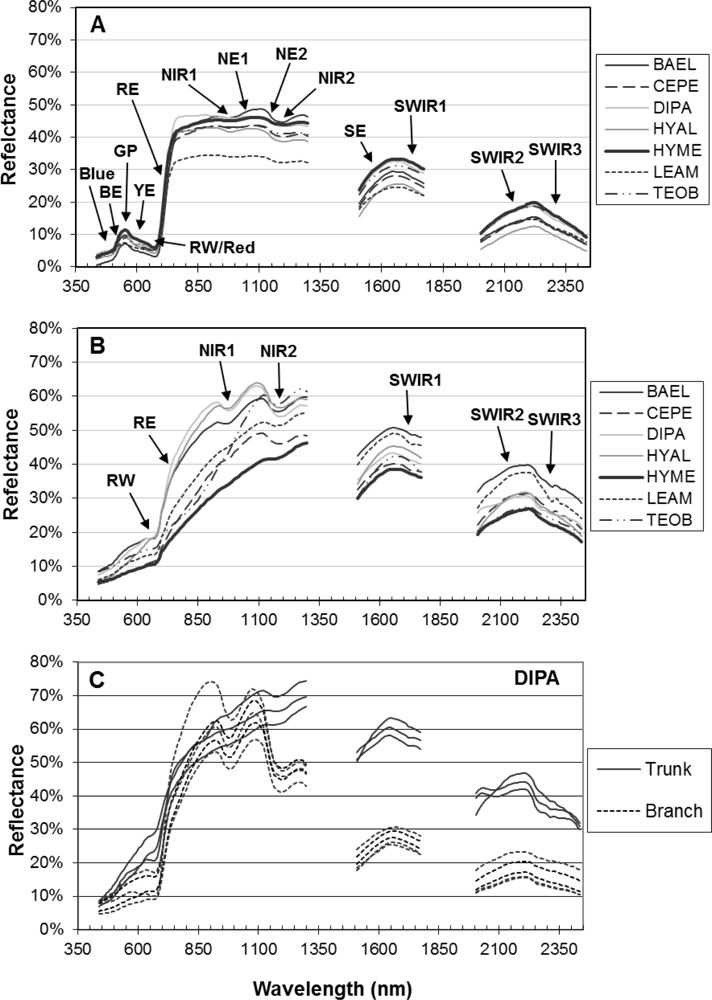
Figure 1.
Laboratory reflectance spectra for study species. In (A,B), lines represent average spectra for species, with codes Balizia elegans (BAEL), Ceiba pentandra (CEPE), Dipteryx panamensis (DIPA), Hymenolobium mesoamericanum (HYME), Hyeronima alchorneoides (HYAL), Lecythis ampla (LEAM), and Terminalia oblonga (TEOB); labels point to spectral features considered in this study, with codes defined in 3rd table in Section 3.5. (A) Mean spectra of leaf samples [16 BAEL, 15 CEPE, 30 DIPA, 30 HYAL, 23 HYME, 14 LEAM, and 24 TEOB], (B) mean spectra of bark samples [15 BAEL, 9 CEPE, 10 DIPA, 5 HYAL, 8 HYME, 12 LEAM, and 7 TEOB], and (C) individual DIPA trunk (n = 5) and branch (n = 5) bark spectra.
Leaf and bark laboratory spectra were convolved to HYDICE band center positions (161 bands) using full width at half maximum information for each HYDICE band. Hyperspectral metrics (Section 3.5) were calculated from convolved bark and leaf spectra. For SMA applied to image data, we sought a more exhaustive bark spectral library and included spectra from the study species as well as 24 field spectra. Bark field spectra came from tree trunks measured at La Selva at 9:30–10:00 am local time in August 2002. The ASD FieldSpec sensor with 8° fore-optic was held about 1 m from the trunk and measured radiance was converted to reflectance using an in situ white Spectralon® calibration panel in full sun.
3.5. Calculation of Hyperspectral Metrics
Hyperspectral metrics are summarized in Table 1. Definitions and procedures for calculating these metrics are presented below.

Table 1.
Summary of hyperspectral metrics organized by methods (in bold) and dominant spectral features and region (in italics).
Narrowband, ratio-based indices were calculated using formulas in Table 2 applied to reflectance spectra at tissue, pixel and crown scales. The HYDICE bands chosen for the indices were closest to those in the formulas presented in the literature.
Table 2.
Formulas for narrow-band, ratio-based indices (ρ is reflectance at a specific wavelength in nm).
Derivative analysis was used to measure the wavelength position and magnitude of the blue edge (BE), green peak (GP), yellow edge (YE), red well (RW), red edge (RE), NIR water absorption edges (NE1 and NE2), and the SWIR1 edge (SE) (Table 3; Figure 1(a)). Derivatives for these features were calculated using a polynomial-fitting technique [75]. Reflectance data were retrieved for all bands in the region covering a spectral feature (e.g., red edge) and a function was then fit to the wavelength and reflectance values according to a polynomial equation and a least-squares minimization:
where ρ represents the HYDICE reflectance values at λ wavelengths within the absorption feature (Table 3), n is the polynomial order, and α represents the n fitted polynomial constants. A continuous derivative spectrum for each feature was then calculated using the fitted polynomial function and used to estimate the wavelength of the local minima or maxima for the edge features, corresponding to the inflection point in the original reflectance domain. Similarly, the wavelength position at which the derivative was zero identified the GP and RW features—the peak and well in the reflectance domain, respectively. The magnitude of the derivative (i.e., reflectance slope) was retrieved at edge inflection wavelengths, while reflectance was retrieved at the GP and RW wavelengths [57].
Table 3.
Definition of spectral features analyzed (See Figure 1(a)).
Green (photosynthetic) vegetation metrics based on derivative area were calculated following methods outlined in Elvidge and Chen [45] and Gong et al. [57]. First-order derivatives of spectra were calculated using a 3-point, Lagrangian interpolation and then the total area under the derivatives was calculated for the blue edge (BE-DArea; called SDB in [54]), yellow edge (YE-DArea; called SDY in [57]) and the red well-red edge (RE-DArea; called 1DL_DGVI in [45]. If a derivative metric did not produce a reasonable value due to an absent or very weak absorption feature, then 0 values were assigned.
Using continuum-removal methods adapted from Pu et al. [76], we calculated several “absorption-based” metrics, including the maximum depth (D), width (W), area (A—maximum depth times width) and asymmetry (As—ratio of area left of absorption center, to area right of absorption center) for the absorption features listed in Table 3: Blue, Red, NIR1, NIR2, SWIR1, SWIR2 and SWIR3. If one of these absorption-based metrics did not produce a reasonable value due to an absent or very weak absorption feature, then 0 values were assigned.
We calculated EWT using a Beer-Lambert light-extinction model, with parameters fit to reflectance data between 865 and 1,065 nm using a non-linear least-squares minimization routine [64]. The spectrum of water absorption coefficients required by this technique was interpolated to HYDICE wavelengths from data in Palmer and Williams [77].
Pixel- and crown-scale spectra were unmixed using a three-endmember SMA model [69] composed of GV, NPV and photometric shade (uniform reflectance of zero). Our original goal was to use image endmembers as they included the signal artifacts in the HYDICE data (e.g., radiometric calibration, atmospheric contamination, bi-directional reflectance). Furthermore, we sought GV and NPV image endmembers (pixel scale) that were from of our study species and as spectrally pure as possible given signal artifacts, sub-pixel spectral mixing, and lack of independent reference data. This was accomplished by plotting pixel-scale spectra from our study crowns in a red versus NIR scatter plot. Thirteen pixels with relatively low red and high NIR reflectance were selected for GV and nine pixels with relatively high red and low NIR were selected for NPV. To reduce noise and make these endmembers more representative across species, we averaged the GV and NPV pixel spectra, respectively, to create one spectrum per endmember. Our NPV image endmember appeared to be spectrally contaminated by GV as it had many characteristics of leaves (i.e., red chlorophyll and NIR water absorption features); and thus, we sought more spectrally-pure NPV endmembers by including a library of 90 field and laboratory spectra in the analysis. An NPV endmember was selected from the library using the criteria that it yield a low model RMSE and provide physically reasonable fractions when combined with the image GV endmember to unmix the image NPV endmember [69]. The final NPV reference endmember ultimately selected was from a lichen-covered tree trunk spectrum acquired in the field at La Selva.
3.6. Species Classification and Ranking of Metric Importance with Random Forests
The Random Forests (RF) classifier [11,38,78–80] was used to identify species from their hyperspectral metrics. The RF classifier is an ensemble of decision trees which have been trained on bootstrapped samples of the reference data. For each tree, node splits are determined with random samples of the predictor variables. For classification of a sample, the class is determined by the majority vote of the ensemble of trees. Roughly 2/3 of the reference data are sampled with replacement to build each tree, while 1/3 of the reference data are withheld from tree construction (called “out-of-bag”, or OOB samples) and yield an unbiased estimate of accuracy [38,78]. The RF classifier also tracks predictor variable importance, which is calculated as a decrease in overall or class-level classification accuracy when the variable is permuted in the OOB samples. We used the importance measure from RF at each scale to rank hyperspectral metrics.
We implemented the RF classifier using the R statistical program (V. 2.11.1) [81] and the randomForest package (V. 4.5–34) [82]. Parameters used for all RF analysis were: 1999 trees, a minimum of 3 samples in terminal nodes, and sqrt(p) as number of variables randomly sampled as candidates at each split, where p is number of variables. RF classification was performed with hyperspectral metrics from tissue- (bark, leaf), pixel- and crown-scale spectra, with the following sets of metrics: (1). indices; (2). absorption-based; (3). derivative; (4). SMA fractions (pixel and crown scale only); and (5). all available metrics. We devised a second method of RF to exclude highly correlated metrics within each set—referred to as “reduced correlation” metrics. At each scale, metrics were first ranked in importance from the standard RF procedure applied to all variables in a set. A subset of metrics with reduced correlation for each set was found by sequentially adding metrics to a selection set, moving in order i from high to low importance. At each step, the i-th metric was compared against the preceding metrics in the selection set using the Spearman rank correlation coefficient. The i-th metric was then added to the selection set if had a correlation less than |0.85| with all other metrics in the selection set.
A second ITC classification was developed called “pixel-majority”, which is similar to the “object-based” procedure used in Clark et al. [8]. First, pixels from crowns not used in training the pixel-scale RF were selected as a test dataset. Metrics from test pixels were then used to predict their species class based on the pixel-scale RF (full correlation or reduced correlation, sets 1 through 5). The species of each tree crown was then assigned based on the majority class of its classified test pixels.
Pixel, crown and pixel-majority classifications were performed with spectra derived from all pixels within crowns and with sunlit pixels from crowns, as per Clark et al. [8]. The RF based on sunlit-only pixels generally had lower accuracy than when using all pixels, and so results with sunlit-only pixels are not presented.
4. Results
4.1. Random Forests Classification Results
There were no statistically significant differences in accuracy when using correlated or reduced-correlation metrics with any variable set (Table 4). Classifications using all available (set #5), reduced-correlation metrics, had 3.3% and 1.4% less accuracy than with correlated metrics for leaves and leaves with bark, respectively (Table 4). However, bark, pixel-scale and crown-scale overall accuracy was 1.5%, 1.3% and 0.9% higher with reduced-correlation metrics, respectively.
Table 4.
Overall classification accuracy with Random Forests for leaves, bark, pixels, and mean crown spectra. Pixel majority is the majority vote of classified test pixels within crowns. Classifications were with full and reduced correlation in metrics from each set (Section 3.6). Arrows represent direction of change in overall accuracy between full and reduced correlation (no changes were significant at α = 0.05).
Indices, absorption-based and derivative metrics had similar overall performance within scales (tissue, pixel, crown), although indices performed better than the other sets for leaf spectra and worse for bark spectra (Table 4). At pixel and crown scales, SMA fractions had the lowest accuracy. Using all available metrics (set #5) in RF consistently produced the highest overall accuracies. Since we wanted to find the best metrics for species identification, regardless of technique for deriving the metric, we focused our analysis on set #5—all variables. Our results show that RF accuracy is not significantly affected by correlated variables, which supports findings in other studies [38,78]; the RF classifier is able to efficiently select the best predictor variables out of a large set of correlated variables, without an optimization step. However, we sought to describe metrics that provided complementary rather than redundant information content; and, since there was a slight (non-significant) improvement in overall accuracy with set #5, reduced-correlation metrics at the operational scale of the pixel or crown, our remaining results will mostly highlight this set.
Laboratory leaf-scale metrics had the best overall accuracy (86.8%) relative to bark, pixel and crown scales (Table 4: leaves, all metrics). Class producer accuracy ranged from 73.9% to 100%, while user accuracy ranged from 76.9% to 100% (Figure 2). Confusion between HYME and TEOB was the main reason for lower accuracy. The RF with bark spectral metrics had 12.6% lower overall accuracy than with leaves (Table 4: bark, all metrics). Combining leaf and bark metrics together yielded an 84.9% overall accuracy. Excluding atmospheric, multiple-scattering and other effects on reflectance, this level of analysis may be similar to using an airborne hyperspectral sensor with ultra-high spatial resolution (i.e., centimeters), especially in a low LAI crown—some pixels in the IFOV will be dominated by leaves, while other pixels by bark. Mixing leaf and bark spectra together increases spectral variability within and among species, and some misclassifications of species increase, yet in general, the RF classifier is able to accommodate this variability while maintaining high overall accuracy.
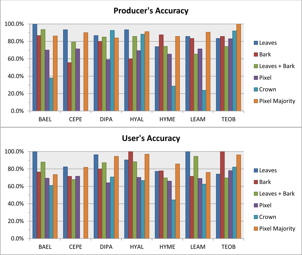
Figure 2.
Producer’s and User’s accuracy for the seven study species using the Random Forests classifier with leaf, bark, pixel and crown spectral metrics. The “pixel majority” accuracy is a majority of vote of within-crown pixels (Section 3.6).
Pixel- and crown-scale metrics from airborne hyperspectral data had lower overall accuracy than for tissue-scale metrics, regardless of set used (Table 4). At the crown scale, overall accuracy using all metrics was only 70.6%, Producer’s accuracy for BAEL, HYME and LEAM was <36%, and no species had User’s accuracies over 82% (Figure 2). No CEPE crowns were correctly classified (0.0% User’s and Producer’s accuracy), possibly due to low sample size (n = 10). The pixel-majority technique for classifying ITCs greatly improved overall accuracy by 16.8% and the classification had less inter-species confusion relative to the crown-scale technique—Producer’s and User’s accuracies were >71% in all classes (Figure 2, Table 5). Confusion was mostly among DIPA, LEAM and BAEL, which were species with low LAI at the time of image acquisition. On average, those ITCs that were correctly classified had 75.6% of their within-crown pixels correctly classified (online supplemental Table S1). However, some ITCs had considerable pixel confusion and could still be correctly classified; in one case, a BAEL crown was correctly classified with only 26.8% of its pixels correctly classified. Of the 26 incorrectly classified ITCs, the incorrect majority class was on average 58.2% of the pixels, but was over 70% of the pixels for individuals in four species (BAEL, DIPA, HYAL, LEAM).
Table 5.
Error matrix for pixel-majority classification using variable set #5 with reduced correlation (Kappa = 0.85).
4.2. Important Hyperspectral Metrics for Identifying Species
The RF importance of all hyperspectral metrics at tissue, pixel and crown scales, without filtering for correlation, is shown graphically in Figure 3. The rankings of metrics, with full and reduced correlation, are available in the online supplement (Tables S2 and S3), while we describe the top-ten important metrics with reduced correlation across scales below (Table 6). Mean and coefficient of variation for metrics from all species and scales are available in the online supplement (Table S4).
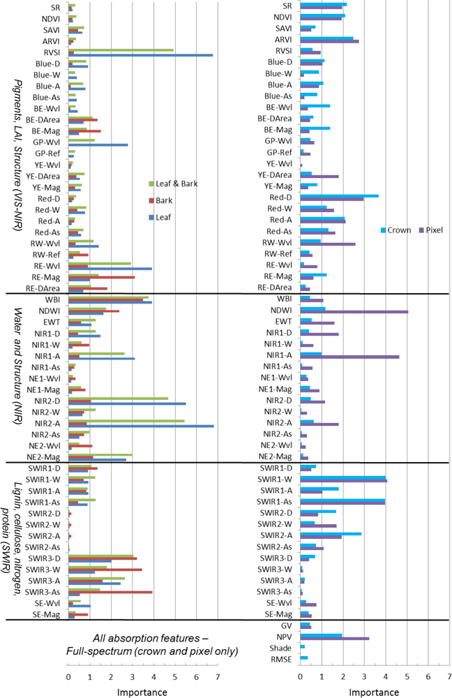
Figure 3.
Importance of leaf, bark, pixel and crown spectral metrics from Random Forests (Section 3.6). All metrics (variable set #5) were included in the Random Forests without considering metric correlation.
Table 6.
The ten most important hyperspectral metrics from Random Forests for classifying the study species at tissue (bark, leaves), pixel and crown scales. Results are for variables with reduced correlation from set #5, with importance ranked high to low based on mean decrease in overall accuracy (Section 3.6).
4.2.1. Important Metrics in VIS to NIR
In leaves, the most important VIR-NIR metrics included RE-Wvl, RVSI, GP-Wvl and ARI2 (Table 6, leaves). The RVSI and RE-Wvl metrics had higher values for BAEL and DIPA leaves relative to the other species (Figure 4). For bark, important metrics were BE-Mag and RE-Mag (Table 6, bark). The median RE-Mag for BAEL and DIPA bark was higher than other species (Figure 4). When leaf and bark metrics were combined in the RF, the important VIS-NIR metrics were more similar to those used at leaf scales, except the PRI entered and GP-Wvl dropped out of the top 10 metrics (Table 6, leaves and bark).
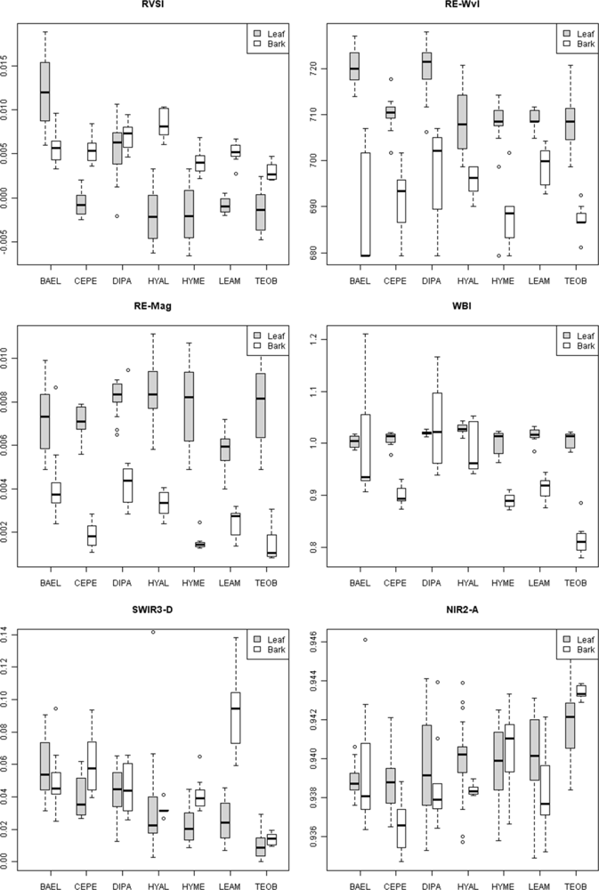
Figure 4.
Box and whisker plots of median values for selected spectral metrics from leaves and bark for the seven study species.
At the pixel scale, important metrics were ARI2, PRI, and RW-Wvl (Table 6, pixels). There was relatively high variation in RW-Wvl within species, and the distribution tended to be bi-modal (Figure 5, lower outliers in box plots) for DIPA, HYME, LEAM and TEOB. This is an example where a non-parametric classifier, such as RF, has a distinct advantage as decision rules can branch at low and high values of the metric and still arrive at the same species. The red absorption feature was important at crown scales (Red-D, RW-Wvl, RE-Mag), as was the blue edge (BE-Wvl, BE-Mag) (Table 6, crown). At the pixel scale, the Red-D metric had relatively low values with high variation for species with low leaf cover (BAEL, DIPA and LEAM), while species with higher leaf cover had high and less variable Red-D (Figure 5). At the crown scale, Red-D was also relatively low for species with low leaf cover and high for species with higher leaf cover. There was much less variation within species (Figure 5) and among species (Table S4, C.V.) at the crown vs. pixel scales, as pixel spectra were averaged to form crown-scale spectra before calculating metrics, thereby reducing finer-scale variability.
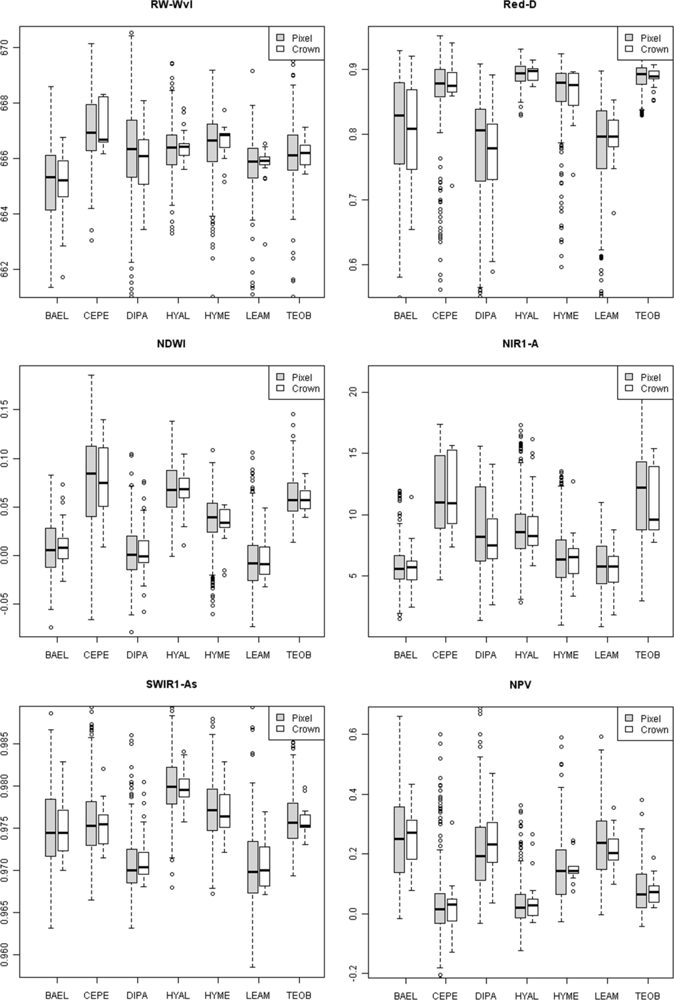
Figure 5.
Box and whisker plots of median values for selected spectral metrics at pixel and crown scales for the seven study species.
4.2.2. Important Metrics in NIR
For leaves, the area of the NIR1 and NIR2 absorption features and WBI were important (Table 6, leaves) water-sensitive metrics for separating species, while WBI, NIR1-W, NE2-Mag, and NE2-Wvl were important metrics for bark. Bark WBI was highest for BAEL, DIPA and HYAL, but with considerable within species variance, and lowest for TEOB (Figure 4). Surprisingly, the WBI from leaves did not have strong median differences among species, but its utility may have been from relatively low variance within species. In contrast, leaf NIR2-A had relatively high within-species variance, but clearer differences in median values among species (Figure 4). For example, NIR2-A for TEOB was relatively high.
At pixel and crown scales, NDWI and NIR1 area were top-ranking metrics, while WBI and NIR2 absorption metrics had much less importance (Figure 3, Table S3, Table 6: pixels, crown). Greater pixel-level water absorption was observed in broad-leaved species that were leaf-on—CEPE, HYAL, and TEOB (Figure 5, NDWI, NIR1-A).
4.2.3. Important Metrics in SWIR
The absorption-based properties of SWIR3 (area, depth, width, asymmetry) were all relatively important for distinguishing species at tissue scales, especially for bark spectra (Figure 3). For example, LEAM bark had distinctly high SWIR3 absorption depth, while TEOB bark had low depth (Figure 4: SWIR3-D). The NDLI, which has bands in the range of the SWIR1 feature, was important at tissue scales. The SWIR2 absorption feature was mostly absent at these scales, leading to zero-value metrics that were relatively unimportant in RF (Figure 3, online supplement Table S2). At pixel and crown scales, though, SWIR1 and SWIR2 absorption metrics and the CAI were highly ranked, while SWIR3 metrics were the least important. As an example of differences among species at these scales, low leaf-area DIPA and LEAM had low SWIR2-As, while high leaf-area HYAL had high SWIR-As (Figure 5).
4.3. General Chemical-Spectral Differences between Leaves and Bark
There are few studies that have analyzed tropical rainforest bark spectral characteristics, and so our data present a unique opportunity to compare chemical-spectral properties of leaves and bark from the same tree species. Relative to bark, leaf metrics had mean values that were higher for VIS-NIR indices (e.g., NDVI, SR, CRI1, CRI2) and blue and red absorption metrics (e.g., Blue-A and Red-A) (online supplement Table S4). Blue and red absorption increased the magnitude (slope) of blue, yellow and red edge features in leaves. In bark, low blue and red absorption meant that there was often no detectable green peak, and so reflectance and wavelength was zero for some specimens, depressing the mean and increasing variance across species. Water indices WBI and NDWI were significantly higher for leaves than bark (p < 0.001, Wilcoxon rank sum test). In particular, the average NDWI for bark was negative, indicating that NIR2 water absorption was absent (i.e., reflectance at 1,239 nm was high relative to reference reflectance at 862 nm). However, the median depth and area of the NIR1 and NIR2 water features were not significantly different for bark than leaves (α = 0.05, Wilcoxon rank sum test), likely because bark had relatively high variation (Table S4). The SWIR indices CAI and NDLI were significantly greater in bark relative to leaves (p < 0.001, Wilcoxon rank sum test). In addition, SWIR1 and SWIR3 absorption features were significantly deeper in bark relative to leaves (p < 0.001, Wilcoxon rank sum test), but not for SWIR2. However, these results indicate that there was less water absorption in bark in the SWIR region relative to leaves, allowing greater expression of SWIR features.
To further explore spectral differences in leaf and bark spectra, we performed PCA applied to their combined metrics. Principal components (PC) #1 and #2 explained 33.9% and 12.2% of the variance, respectively (Figure 6). PC1 had a strong positive correlation (>0.90) with metrics sensitive to photosynthetic pigments and green vegetation structure, Red-D, Red-A, RE-Mag, GP-Wvl, SAVI, ARVI, NDVI, while it had weaker, negative correlation with metrics detecting asymmetrical absorptions, Red-As and YE-DArea, and cellulose (CAI) and lignin (NDLI) features in SWIR. PC2 had strong positive correlation (>0.90) with water absorption metrics—NIR1-D,A, NIR2-A,D, EWT—and weak negative correlations with SWIR1 and SWIR2 absorption metrics. Bark had negative values and leaves had positive values on PC1, respectively (Figure 6). There were clear ellipsoidal groupings of leaves by species in the space defined by PC1 and PC2—on the side of photosynthesis absorptions, with slightly positive (wetter) or negative (more SWIR absorptions, so drier) values along PC2. In contrast to leaves, bark metrics for BAEL, DIPA and HYAL had two distinct groupings along PC2. Visually, the difference in HYAL specimens was not clear from photographs, but for BAEL and DIPA, plate-like bark specimens from the trunks of older trees were lower along this PC2 axis (e.g., more SWIR absorptions, so drier), while branch specimens from younger trees were higher on the PC2 axis (e.g., wetter). The younger branches for both species tended to be mottled with green patches, which accounts for slightly less negative PC1 values (e.g., indicating more photosynthesis-related absorption), while the trunk bark samples were relatively smooth and uniform brown, with more negative PC1 values.
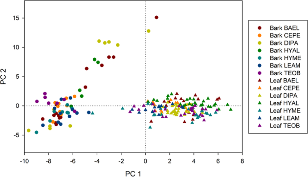
Figure 6.
Principal Components Analysis based on all leaf and bark metrics. Axes are the first and second principal components.
4.4. Crown Structure and Phenology Detected by SMA Fractions
Mean values of spectral mixture fractions from our study crowns were roughly 40% GV, 15% NPV and 44% shade (+1% error) at both pixel and crown scales. Canopies of leaf-off DIPA and LEAM had higher NPV and lower GV fractions (Figure 7). In contrast, leaf-on, broad-leaf species CEPE, HYAL and TEOB had relatively high mean GV and low NPV fractions. However, variability in crown-level proportions of GV, NPV and shade was present within a species. For example, BAEL and HYME (legumes with moderate LAI) had some individuals with NPV and GV fractions similar to leaf-off crowns of DIPA and LEAM, while other individuals of BAEL and HYME had fractions that resembled the crowns of leaf-on, broadleaf species HYAL and TEOB (Figure 7). The NPV fraction was a top-ranked metric in pixel- and crown-scale RF (online supplement Table S3), yet it was removed from the reduced-correlation crown RF due to high correlation with SWIR2-A (Spearman Rank, rs = −0.86; Table 6).
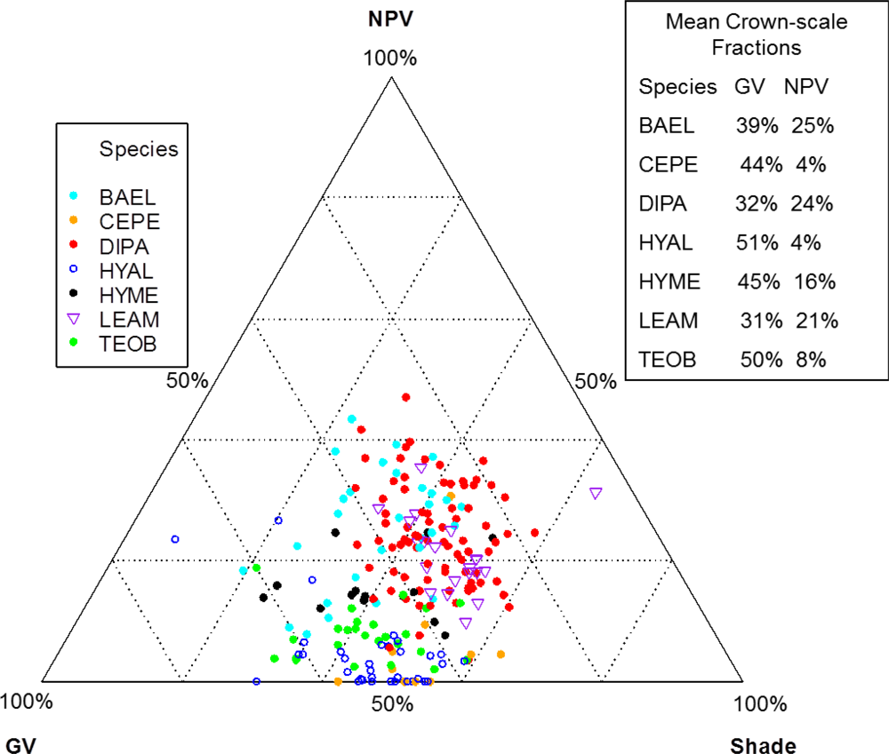
Figure 7.
Spectral mixture analysis fractions of green photosynthetic vegetation (GV), non-photosynthetic vegetation (NPV) and shade for individual tree crowns. Ternary diagram values are the individual tree crown fractions from crown-scale spectra.
The NPV fraction should be inversely correlated with metrics that respond positively to photosynthetic (green) vegetation, such as those that measure the depth, width or area of chlorophyll or water absorption features. This was indeed the case: across species, NPV from pixel spectra (n=37,143) had strong negative correlations with red absorption (Red-D rs = −0.79, Red-W rs = −0.78), and weak negative relationships with water absorption (NIR1-D rs = −0.28, NIR1-W rs = −0.13; NIR2-D rs = −0.35, NIR2-W rs = +0.08). In contrast, with less water absorption in low leaf-area crowns (i.e., low GV), high fractions of exposed NPV correlate with deeper SWIR absorption features. Indeed, we found NPV from pixel spectra had slightly positive (except SWIR3-D negative) correlations with SWIR absorption features (SWIR1-D rs = +0.12, SWIR1-W rs = +0.56; SWIR2-D rs = +0.26, SWIR2-W rs = +0.45; SWIR3-D rs = −0.30, SWIR3-W rs = +0.35; CAI rs = +0.43)
5. Discussion
5.1. Species Phenology Detected by Metrics from Hyperspectral Imagery
Individuals of BAEL, DIPA and LEAM had crowns with relatively high percentages of NPV compared to other species (Figures 5 and 7), which can be attributed to bark tissues exposed to the sensor [25]. The deciduous DIPA and LEAM trees in our study area had low LAI at the time of image acquisition, while individuals of BAEL had relatively high amounts of NPV because of their architectural properties—compound leaves with fine leaflets, sparse arrangement of leaves, and conspicuous white bark mostly free of other organisms. Crowns with low LAI (e.g., DIPA), were easily identified in both the hyperspectral reflectance imagery (Figure 8; natural color) and the images of hyperspectral metrics (Figure 8; SMA fractions, NDWI, NDVI). In the SMA false-color image, crowns with low leaf-area were clearly seen as groups of pixels with high NPV (red) in a matrix of high-GV canopy (green) and high-shade gaps (blue).
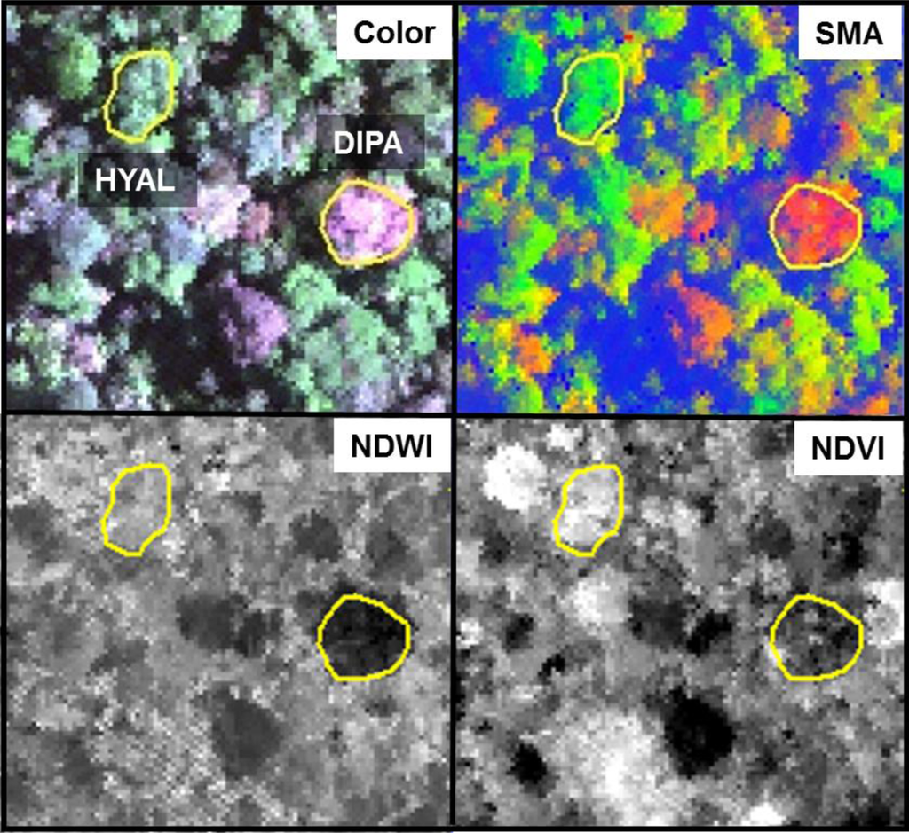
Figure 8.
A 300 × 300-m section of hyperspectral data (center at 10°25′52″N, 84°0′36″W) and derived metrics over individual DIPA and HYAL trees (yellow polygons). The natural color image displays reflectance bands 482, 550, and 679 nm. The spectral mixture analysis (SMA) fraction image displays (Red = NPV, Green = GV, Blue = Shade). Normalized Water Difference Index (NDWI) and Normalized Vegetation Index (NDVI) images show low (black) to high (white) values.
5.2. Species Differences in VIS to NIR Metrics Sensitive to Pigments, Structure and Stress
The RF classifier identified the red-edge as important for discriminating our set of species at tissue scales. The RE-Wvl and RVSI metrics were key variables for leaves. These results are consistent with work by Cochrane [36], Clark et al. [8] and Rivard et al. [34], who also found this region useful for distinguishing leaves from moist tropical forest trees. The shape of the red edge is heavily influenced by photon absorption and florescence from chlorophyll in tissues [15,21]. Research has shown that high concentrations of chlorophyll in leaves widens and deepens red-well absorption and shifts the red-edge inflection point toward longer wavelengths [83]. In our study, BAEL and DIPA had a red edge at longer wavelengths than other species (Figure 4, RE-Wvl), and the red absorption depth (Red-D) was also high for these species, suggesting that relatively high chlorophyll concentration for these species helps distinguish them from other species. The RVSI was designed to detect red-edge curve concavity or convexity relative to a baseline. The index was originally used to track vegetation communities through time, not spectral properties of tissues. We found that leaf-scale RVSI was not well correlated with any other red and red-edge metrics, and the metric does provide unique information for separating species using leaf spectra.
The red-edge magnitude, rather than inflection wavelength, was an important metric for discriminating species using bark spectra. Compared to leaves, bark had low to no chlorophyll and so there was relatively low red-well absorption, increased red-well reflectance (RW-Refl), decreased slope of the red-edge (lower magnitude, RE-Mag), and a shift in the red-edge inflection point toward shorter wavelengths (Figure 1, online supplement Table S4). We found that BAEL and DIPA bark had the highest RE-Mag values, while TEOB bark had the lowest values (Figure 5). BAEL and DIPA bark specimens from young branches were mottled green and a PCA showed they had distinct spectral properties, likely due to photosynthesis and water absorption. An example of the greener branches is shown for DIPA (Figure 1(c)). The branches have well-defined red absorption features and a steeply sloped red-edge, which translates into higher RE-Mag values overall (Figure 1(b), BAEL, DIPA; Figure 4, BAEL, DIPA). In contrast, TEOB bark samples were mostly dark brown with minimal green mottling, and their red-edge had a relatively shallow slope (Figure 1(b), TEOB).
Metrics in the VIS-NIR that were important at the tissue scale were not predictive of metric importance at the pixel and crown scale. At these broader scales, metrics describing the red/chlorophyll absorption feature shape (e.g., depth) and position (e.g., red well wavelength) were important, rather than the red edge. Crown architecture and tree phenology were important factors in determining the amounts and exposure of bark, as well as lichens, bryophytes, epiphytes and other canopy components. High leaf-area species, such as HYAL and TEOB, had high red depth (Red-D), presumably due to chlorophyll absorption; these species also had relatively high NIR reflectance, likely due to multiple scattering among transmittant leaves [8], and consequently their SR and NDVI values were relatively high (Figure 8). In contrast, low leaf-area BAEL, DIPA and LEAM had a higher concentration of bark in the sensor’s IFOV, which translated into relatively high red-well reflectance due to lower chlorophyll absorption and low NIR reflectance due to less photon scattering; and thus, Red-D, SR, and NDVI values were relatively low for these species.
5.3. Species Differences in NIR Metrics Sensitive to Water and Structure
The NIR1 and NIR2 water-sensitive metrics, especially area, were important for distinguishing species leaves. Internal leaf structure, such as the air-cell wall interfaces in the spongy mesophyll, scatters NIR photons, increasing the expression of absorption features [21]. Species differences in water absorption depth, width and area may thus result from a combination of factors that affect internal leaf photon scattering and absorption, such as leaf thickness, water content and the distribution of air-cell wall interfaces.
Bark specimens were generally less wet than leaves, as indicated by significantly lower WBI and NDWI values and clustering of bark on the PC1 axis side that indicated less water absorption. However, there was variability among and within species in water-related metrics. For example, much of the within-species bark variability comes from spectral differences between branch and trunk bark, as seen in VIS-NIR metrics. Our results thus indicate that bark spectral properties can vary considerably within a population of tropical tree species, even on a single individual, without considering increased spectral variance from surface lichens, bryophytes, etc. In temperate forests, Williams [84] found that first-year twig spectra for conifer and hardwood species showed evidence of chlorophyll and NIR water absorption, and the depth of these features decreased considerably in second-year twigs from the conifer species, which were more woody. In our data, it appears that bark chlorophyll and NIR water absorption features are correlated because young branches have relatively more live tissues near the bark surface.
The depth, width and area of NIR water absorption features increased from the centimeter spatial scales of leaf and bark laboratory spectra to the 1.6-m scale of image pixels (Table S4). The depth of these features can be partly attributed to poor radiometric calibration and signal-to-noise in the HYDICE sensor (discussed in Clark et al. [8]). However, the three-dimensional stacking of leaves and branches within the crown, which increases the path length of photons and increases their multiple-scattering and absorption, is expected to accentuate tissue-level chemical and structural properties [12,14,17,23]. Water absorption metrics calculated at pixel and crown scales should thus respond to the combination of water content of GV and NPV tissues and the structural distribution of these tissues within the crown [62–64]. The water absorption signal should be greater with more LAI relative to branch area because leaves tend to be wetter, and they are more transmittive, thereby permitting more photon scattering. This effect can be observed in Figure 5, where a low leaf-area DIPA had relatively low NDWI relative to leaf-on HYAL, and Figure 8, where pixels within DIPA crowns formed dark crowns in the NDWI image. In terms of RF metric importance, species differences in both NIR water absorption metrics were important at all scales. However, pixels and crown RF had more importance for NDWI (targets the NIR2 feature) and NIR1 area, whereas leaf and bark RF gave WBI (targets NIR1 feature) and NIR2 area more importance.
5.4. Species Differences in SWIR Metrics Sensitive to Non-Pigment Chemicals, Water and Structure
Metrics incorporating the area, asymmetry and width of SWIR1 and SWIR2 features were among the top-ranked metrics at pixel and crown scales. While the SWIR3 metrics were important at tissue scales, they were likely less important at pixel and crown scales due to low signal-to-noise in the HYDICE sensor and low reflectance in the region [8,74]. The SWIR1 feature is associated with lignin (primarily), starch, protein and nitrogen absorption and the SWIR2 feature is associated with protein and nitrogen (primarily), starch and cellulose absorption [17]. The SWIR1 and SWIR2 absorption features were detected more in bark vs. leaves: 70% and 15% of bark spectra, 5% and 7% of laboratory leaf spectra, respectively. These results suggest that bark has more of these chemical constituents than leaves, but differences could be related to less SWIR water absorption in bark. Radiative transfer models show that, with closed-canopy tropical forest, photons in SWIR wavelengths do not penetrate deeply into the canopy due to strong water absorption, and thus hyperspectral sensors only sense upper-canopy chemicals [12,20]. However, PLSR models based on leaf spectra from humid tropical forests indicate that SWIR is vitally important for accurately predicting a range of foliar chemicals, such as carbon, phenols, tannins, N, P, and K, as well as water [20,29,31]. In addition, research in chaparral communities showed that SWIR indices lost predictive capacity for bulk canopy lignin and nitrogen when senesced vegetation was included in the analysis [67]. The reason why SWIR1 and SWIR2 metrics were important for species discrimination at pixel and crown scales is thus likely related to LAI variation in crowns. In our pixel-scale data, we found the width of all three SWIR absorption features increased (i.e., broadened) with higher NPV (i.e., lower LAI), while depth only slightly increased for SWIR1 and SWIR2 features. This broadening and slight deepening, appears to have created important species-level differences in SWIR1 feature asymmetry (left to right area ratio), as species with low LAI (DIPA, LEAM) had lower median SWIR1-As (Figure 5). It is not clear why low-LAI crowns have broad SWIR features, as RT models have not considered bark chemical-biophysical interactions. However, we speculate that crowns with lower LAI have less influence by water absorption and more expression of overlapping SWIR chemical absorptions.
5.5. Individual Tree Crown Classification with Random Forests
Our data show that leaf and bark tissues have distinct spectral characteristics as detected by hyperspectral metrics, which translates into higher spectral variability within an individual tree, within a species, and ultimately among species. The relative abundance and arrangement of these tissues in a crown, in turn, will determine the variability of metrics at broader spatial scales, and through seasonal phenological cycles. Given this spatio-temporal variability, spectral metrics do not necessarily have uni-modal distributions within a single crown, let alone among individuals in a species, and especially not at pixel sizes of VHR sensors.
A decision tree classifier is an intuitive technique for discovering multiple, non-linear pathways through the metrics to arrive at species labels. We found the tree-based RF classifier particularly useful for species discrimination based on spectral metrics in that it: (1) could handle non-parametric data and a multi-modal decision space; (2) generated hundreds of decision trees through random sampling of the data, instead of relying on just one—potentially overfit—model; (3) used all data for training, yet produced an unbiased measure of accuracy based on a cross-validation approach (OOB); (4) discovered the best metrics to use in the classification, without an optimization step; and, (5) produced a rank of important metrics, which we used for inferring chemical and structural differences among species.
At all spatial scales, the RF classifier had better performance when all metrics were included, through iterative random sampling, the most important metrics are selected in decision rules (Table 4). The top-ten metrics in RF at all scales were derived from narrowband indices, absorption-based and derivative techniques (Table 6); and, VIS, NIR and SWIR spectral features all appeared in these top-ranking metrics. This result concurs with other studies using PLSR and leaf spectra [28,29,31] in that the whole 400–2,500 nm spectrum should be considered when classifying tree species from hyperspectral imagery.
Leaf spectral metrics could discriminate species with 87% overall accuracy. Overall accuracy dropped only 2% when metrics from leaf and bark samples were combined in a single RF—which is impressive considering the extreme spectral variability introduced by bark. At the 1.6-m scale of our imagery, the RF classifier based on all metrics from randomly-sampled pixels within crowns had roughly the same performance (∼70% overall accuracy) as when using the average spectra from crowns, however the pixel-majority classification had much better accuracy, at 87% overall. The 88% Producer’s and 90% User’s accuracies for DIPA from the pixel-majority technique (Table 5) are encouraging for mapping this species of high conservation value [8]. Confusion of DIPA with BAEL and LEAM (Table 5) was likely due to similar LAI from architecture and phenology, resulting in fractions of GV and NPV tissues and comparable photon scattering environments that created similar responses in our chemical-structure metrics.
The pixel-majority technique can accommodate within-crown spectral variation from VHR imagery, such as from pixels with a mix of bark, leaf, liana or epiphyte spectral properties, and still identify the correct species of the ITC. On average, correctly classified ITCs had 75% of their within-crown pixels correctly classified. Some crowns received the correct species label, but with only a fourth of the pixels correctly classified, indicating that ITCs can have high internal spectral variability. The 72% overall accuracy of the pixel-scale RF shows that it can handle some spectral variation among pixels within a species. By taking the majority vote of pixels within ITCs, the error from any misclassified pixels within a crown is minimized. However, a major caveat is that our data only include seven species. The pixel-scale RF performance, and thus crown pixel-majority accuracy, would likely decrease in mapping an entire tropical rainforest due to increased spectral diversity from hundreds of species.
5.6. Comparison with Past Research
The pixel-majority approach to classifying ITC tree species with spectral metrics was superior to using crown-scale metrics (87.4% vs. 70.6%). In our previous analysis [8], which used the same hyperspectral data as a starting point, we found that optimally-selected reflectance bands and a LDA classifier had 92.1% classification accuracy with crown-scale spectra, while the LDA pixel-majority classification had 83.6% overall accuracy. The LDA classifier also achieved better overall accuracy with leaf- and pixel-scale reflectance data [8]. Why did LDA and reflectance data outperform Random Forests and spectral metrics at leaf, pixel and crown scales? The LDA classifier considers all predictor variables simultaneously to build a decision space using predictor variable covariance. In contrast, the decision space of a tree in RF is built one variable at time, and decisions at terminal nodes are dependent upon those at higher nodes. The decision tree is thus more susceptible to misclassification errors when data variability causes many different possible splits. The RF classifier attempts to minimize errors from a single decision tree through random sampling, generating hundreds of decision trees, and deriving the class label from a majority vote; and thus, RF should be fairly robust in the face of spectral variability. Another factor to consider is the difference in using reflectance data versus spectral metrics derived from reflectance. Illumination can influence spectral differences among species, and it is best captured by reflectance spectra as opposed to hyperspectral metrics, which minimize brightness variation from continuum removal, derivative analysis or band ratios. If illumination was the dominant factor in distinguishing species, we would have expected the SMA shade fraction to be among the top metrics in RF. Instead, Shade ranked 31 and 26 out of 66 metrics in pixel and crown RF, respectively (online supplement Table S3). These results suggest that illumination variation is not a principal factor in discriminating species. In general, our metrics were not well correlated with shade (data not shown), indicating that species were mostly separated according to chemical absorptions and structure rather than illumination.
In many respects, our comparison of the LDA and RF classifiers for species discrimination is imperfect given the small sample size and lack of an independent test dataset. Our previous results with LDA are likely positively biased because they rely on band optimization using all available data and “leave-one-out” cross validation, whereas in RF there is no optimization step, 1/3 of the data can be randomly chosen and held out of each tree for accuracy assessment, and there were 1999 decision trees—as opposed to one LDA classifier. Given its ability to handle intra- and inter-class spectral variability, the RF classifier may prove more robust and less prone to over-fitting when applied to datasets with even higher spectral variability, as when including more species or using higher spatial resolution imagery.
5.7. Recommendations for Future Research
What the LDA and RF classifiers did find in common was that spectral information should come from across the VIS, NIR, and SWIR regions [8]. Several of the most important reflectance bands and spectral metrics were found in NIR and SWIR; and thus, we recommend that future species discrimination research use hyperspectral sensors that cover the full 400 to 2,500 nm range. Engineering improvements in sensor signal-to-noise in the SWIR region should lead to a greater ability to discriminate species with distinct phenology or structure. The research community would greatly benefit from more datasets from technologically-advanced sensors flown over tropical forests, especially from sites with high species diversity, various land-cover types, and rich field data.
There are several limitations to our analyses in this and the Clark et al. [8] study that could be addressed through future research. Ideally, we would have used an independent validation dataset instead of OOB or cross-validation accuracy statistics. However, tropical forests typically have high species diversity, but with low population densities, making it difficult to collect enough samples for training, let alone for testing. Partly due to sampling issues, we limited our analyses to seven out of hundreds of tree species that occur at our study site, and individuals analyzed were relatively large, canopy-emergent trees with well-exposed crowns. An operational approach to mapping target species across a forest canopy will need to include a much broader range of species, including those with smaller and canopy-level crowns. For a pixel-majority technique, an appropriate image segmentation algorithm must be found to delineate crown objects [6,9,10], a task that may benefit from canopy structure information provided by coincident lidar data. Alternatively, dominant species or species richness mapping may be more successful through per-pixel estimation techniques [60,70].
Another limitation of our study was that we had no tissue chemical assays from our study species, and so our discussion of chemical properties detected by spectral metrics is speculative. A more instructive study would entail linking chemical compounds in leaves and other canopy components to airborne hyperspectral data, preferably acquired near the same time. Unfortunately, this was not possible in our study as we analyzed the imagery many years after it was acquired. Recent research with high-fidelity spectral, chemical and structure measurements from leaves of tropical forest trees has made great strides in scaling species chemical-spectral diversity from the leaf to canopy scales with modeling techniques [12,28–31].
Many of our results indicate that leaf phenology is a major factor in distinguishing species, as it changes the chemical-structural properties that influence their spectra. Here we have inferred phenological state and associated structural properties of trees based on field data and observations not directly linked to our individual study trees. This limits the conclusions we can draw from our results. We recommend that future studies acquire ITC estimates of crown structure (e.g., leaf and branch area) and other biological information, like liana cover, epiphyte cover, and flower density through either field observations or interpretation of VHR color imagery. Both tissue chemical assays and phenological data, acquired at the time of image acquisition, will permit a deeper understanding of the within- and among-species spectral variation that is expressed in a crown’s reflectance spectra or hyperspectral metrics.
6. Conclusions
In this study we explored a method to classify tropical rainforest tree species from full-range (400–2,500 nm) hyperspectral data acquired at tissue, pixel and crown scales. We focused on seven canopy-emergent species (Balizia elegans, Ceiba pentandra, Dipteryx panamensis, Hymenolobium mesoamericanum, Hyeronima alchorneoides, Lecythis ampla, and Terminalia oblonga) from a site in Costa Rica. Our study was unique for hyperspectral research focused on tropical species discrimination in several ways. First, at the tissue scale we analyzed bark spectra in addition to a traditional analysis of leaf spectra. Second, we used the non-parametric Random Forests classifier, which had not been previously used for tropical forest species classification. Finally, rather than use reflectance bands for predictor variables, we used a suite of hyperspectral metrics that should respond to vegetation chemical (e.g., pigments, water, lignin, cellulose, and nitrogen) and structural properties (e.g., LAI). Some of the narrowband indices were adaptations from broad-band formulations, yet most metrics used were specific to hyperspectral data. In particular, derivative and absorption-based indices relied on band contiguity, a unique characteristic of hyperspectral data, to describe spectral shape and extract information.
Metrics exhibited multi-modal data distributions, yet Random Forests was well-suited to this classification problem across scales. For tissue spectra measured in the laboratory, overall accuracies were 86.8% for leaves and 74.2% for bark, respectively. One important finding was that overall accuracy was only slightly less for leaf and bark metrics combined (84.9%) than with leaves alone; considering the different chemical-structural effects of these tissues on increased within- and among-species spectral variability, this result is an impressive testament to Random Forests ability to handle multi-modal distributions. With airborne hyperspectral data, overall accuracies for individual tree crowns were 71.5% for pixel spectra and 70.6% crown-mean spectra. Using the RF classifier and an object-based pixel-majority vote achieved an impressive 87.4% overall accuracy, and confusion was mainly between low leaf-area species.
Since the RF classifier can rank metrics by importance, it was a powerful tool to decipher the fundamental chemical, structural and phenological factors that drive spectral differences among species. In general, we found that metrics sensitive to chemicals and structure across the visible to shortwave infrared (SWIR) spectrum were useful to discriminate species from centimeter scales of leaf and bark tissue to pixel or crown scales measured by the airborne sensor, although the important metrics varied with scale. For example, the top-three metrics chosen by Random Forests for classifying leaves and bark were sensitive to near infrared (NIR) water absorption (NIR2-A, WBI) and a SWIR feature (SWIR3-D); the pixel-scale top-three metrics were also sensitive to NIR and SWIR absorption features (NIR1-A, SWIR1-As) as well as an anthocyanin feature (ARI2) in the visible spectrum; and, the crown-scale top-three metrics were sensitive to SWIR features (SWIR1-W, SWIR2-A) and the red chlorophyll absorption feature (Red-D). We found that variation in leaf and bark metrics is explained primarily along an axis of red absorption related to photosynthesis in leaves and another axis distinguishing SWIR chemical and NIR water absorption features, attributed to photosynthetic (wet) properties of younger green bark in some species. At pixel and crown scales, tree structure and phenology at the time of image acquisition were driving factors on spectral separability of species.
Much more research is needed to achieve operational mapping of tropical forest tree species, and our suite of hyperspectral metrics and object-based classification approach should be tested with many more species, at other sites, and with improved sensors. However, our results show that our seven tropical tree species were reliably discriminated with hyperspectral metrics selected by the Random Forests classifier, whose strength lies in its ability to accommodate the within-species spectral variability found in tropical forests. Our results also corroborate those from other studies that have found statistical separation of tropical forest species based on analysis of hyperspectral data [8,22,34,36,37]. Adding to this, there is mounting evidence that tropical tree species have unique leaf chemical signatures that manifest as distinct hyperspectral signatures [28–31], and overall canopy species richness may track spectral-chemical diversity measured by full-range hyperspectral sensors [12,28]. Therefore, despite the many challenges that tropical rainforests present to operational species mapping, we conclude that imaging spectroscopy is the most credible technology for attaining this goal.
Acknowledgments
This work was supported with grants to Clark by NASA Headquarters under the Earth System Science Fellowship Grant NGT5-30436 and a California Space Grant Graduate Fellowship. NASA’s AVIRIS team at the Jet Propulsion Laboratory provided the ASD spectrometer used for measuring laboratory spectra. Some tree data were from the TREES project, provided by David Clark and Deborah Clark. The long-term monitoring of the TREES Project focal species was made possible by support from National Science Foundation’s LTREB program (most recently LTREB DEB-0640206). We thank Leonel Campos, William Miranda and Catherine Cardelús for field assistance in collecting bark samples.
References
- Wilson, E.O.; Peter, F.M. (Eds.) Biodiversity; National Academies Press: Washington, DC, USA, 1998.
- Pan, Y.; Birdsey, R.A; Fang, J.; Houghton, R.; Kauppi, P.E.; Kurz, W.A.; Phillips, O.L.; Shvidenko, A.; Lewis, S.L.; Canadell, J.G.; et al. A large and persistent carbon sink in the world’s forests. Science 2011, 333, 988–993. [Google Scholar]
- Hansen, M.C.; Stehman, S.V.; Potapov, P.V.; Loveland, T.R.; Townshend, J.R.G.; DeFries, R.S.; Pittman, K.W.; Arunarwati, B.; Stolle, F.; Steininger, M.K.; et al. Humid tropical forest clearing from 2000 to 2005 quantified by using multitemporal and multiresolution remotely sensed data. Proc. Natl. Acad. Sci. USA 2008, 105, 9439–9444. [Google Scholar]
- Barbier, N.; Couteron, P.; Proisy, C.; Malhi, Y.; Gastellu-Etchegorry, J.-P. The variation of apparent crown size and canopy heterogeneity across lowland Amazonian forests. Global Ecol. Biogeogr 2010, 19, 72–84. [Google Scholar]
- Clark, D.B.; Castro, C.S.; Alvarado, L.D.A.; Read, J.M. Quantifying mortality of tropical rainforest trees using high-spatial-resolution satellite data. Ecol. Lett 2004, 7, 52–59. [Google Scholar]
- Palace, M.; Keller, M.; Asner, G.P.; Hagen, S.; Braswell, B. Amazon forest structure from IKONOS satellite data and the automated characterization of forest canopy properties. Biotropica 2008, 40, 141–150. [Google Scholar]
- Cho, M.A.; Debba, P.; Mathieu, R.; Naidoo, L.; Aardt, J.V.; Asner, G.P. Improving discrimination of savanna tree species through a multiple-endmember spectral angle mapper approach: Canopy-level analysis. IEEE Trans. Geosci. Remote Sens 2010, 48, 4133–4142. [Google Scholar]
- Clark, M.L.; Roberts, D.A.; Clark, D.B. Hyperspectral discrimination of tropical rainforest tree species at leaf to crown scales. Remote Sens. Environ 2005, 96, 375–398. [Google Scholar]
- Féret, J.-B.; Asner, G.P. Tree species discrimination in tropical forests using airborne imaging spectroscopy. IEEE Trans. Geosci. Remote Sens 2012, in press.. [Google Scholar]
- Lucas, R.; Bunting, P.; Paterson, M.; Chisholm, L. Classification of Australian forest communities using aerial photography, CASI and HyMap data. Remote Sens. Environ 2008, 112, 2088–2103. [Google Scholar]
- Naidoo, L.; Cho, M.A.; Mathieu, R.; Asner, G.P. Classification of savanna tree species, in the Greater Kruger National Park Region, by integrating hyperspectral and LiDAR data in a Random Forest data mining environment. ISPRS J. Photogramm 2012, 69, 167–179. [Google Scholar]
- Asner, G.P. Hyperspectral Remote Sensing of Canopy Chemistry, Physiology, and Biodiversity in Tropical Rainforests. In Hyperspectral Remote Sensing of Tropical and Sub-Tropical Forests; Kalácska, M., Sánchez-Azofeifa, G.A., Eds.; CRC Press: Boca Raton, FL, USA, 2008; Chapter 12; pp. 261–296. [Google Scholar]
- Clark, M.L. Identification of Canopy Species in Tropical Forests Using Hyperspectral Data. In Hyperspectral Remote Sensing of Vegetation; Thenkabail, P.S., Lyon, J.G., Huete, A., Eds.; CRC Press: Boca Raton, FL, USA, 2011; Chapter 18; pp. 423–445. [Google Scholar]
- Asner, G.P. Biophysical and chemical sources of variability in canopy reflectance. Remote Sens. Environ 1998, 64, 234–253. [Google Scholar]
- Ustin, S.L.; Gitelson, A.A.; Jacquemoud, S.; Schaepmand, M.; Asner, G.P.; Gamon, J.A.; Zarco-Tejada, P. Retrieval of foliar information about plant pigment systems from high resolution spectroscopy. Remote Sens. Environ 2009, 113, S67–S77. [Google Scholar]
- Gao, B.C.; Goetz, A.F.H. Column atmospheric water-vapor and vegetation liquid water retrievals from airborne imaging spectrometer data. J. Geophys. Res.-Atmos 1990, 95, 3549–3564. [Google Scholar]
- Curran, P.J. Remote sensing of foliar chemistry. Remote Sens. Environ 1989, 30, 271–278. [Google Scholar]
- Elvidge, C.D. Visible and near-Infrared reflectance characteristics of dry plant materials. Int. J. Remote Sens 1990, 11, 1775–1795. [Google Scholar]
- Kokaly, R.F.; Asner, G.P.; Ollinger, S.V.; Martin, M.E.; Wessman, C.A. Characterizing canopy chemistry from imaging spectroscopy and its application to ecosystem studies. Remote Sens. Environ 2009, 113, S78–S91. [Google Scholar]
- Asner, G.P.; Martin, R.E. Spectral and chemical analysis of tropical forests: Scaling from leaf to canopy levels. Remote Sens. Environ 2008, 112, 3958–3970. [Google Scholar]
- Gates, D.M.; Keegan, H.J.; Schleter, J.C.; Weidner, V.R. Spectral properties of plants. Appl. Opt 1965, 4, 11–20. [Google Scholar]
- Castro-Esau, K. L.; Sánchez-Azofeifa, G. A.; Rivard, B.; Wright, S. J.; Quesada, M. Variability in leaf optical properties of Mesoamerican trees and the potential for species classification. Am. J. Bot 2006, 93, 517–530. [Google Scholar]
- Roberts, D.A.; Ustin, S.L.; Ogunjemiyo, S.; Greenberg, J.; Dobrowski, S.Z.; Chen, J.; Hinckley, T.M. Spectral and structural measures of Northwest forest vegetation at leaf to landscape scales. Ecosystems 2004, 7, 545–562. [Google Scholar]
- Blackburn, G.A.; Milton, E.J. Seasonal variations in the spectral reflectance of deciduous tree canopies. Int. J. Remote Sens 1995, 16, 709–720. [Google Scholar]
- Bohlman, S. Hyperspectral Remote Sensing of Exposed Wood and Deciduous Trees in Seasonal Tropical Forests. In Hyperspectral Remote Sensing of Tropical and Sub-Tropical Forests; Kalácska, M., Sánchez-Azofeifa, G.A., Eds.; CRC Press: Boca Raton, FL, USA, 2008; Chapter 8; pp. 177–192. [Google Scholar]
- Key, T.; Warner, T.A.; McGraw, J.B.; Fajvan, M.A. A comparison of multispectral and multitemporal information in high spatial resolution imagery for classification of individual tree species in a temperate hardwood forest. Remote Sens. Environ 2001, 75, 100–112. [Google Scholar]
- Toomey, M.; Roberts, D.; Nelson, B. The influence of epiphylls on remote sensing of humid forests. Remote Sens. Environ 2009, 113, 1787–1798. [Google Scholar]
- Asner, G.P.; Martin, R.E.; Ford, A.J.; Metcalfe, D.J.; Liddell, M.J. Leaf chemical and spectral diversity in Australian tropical forests. Ecol. Appl 2009, 19, 236–253. [Google Scholar]
- Asner, G.P.; Martin, R.E.; Knapp, D.E.; Tupayachi, R.; Anderson, C.; Carranza, L.; Martinez, P.; Houcheime, M.; Sinca, F.; Weiss, P. Spectroscopy of canopy chemicals in humid tropical forests. Remote Sens. Environ 2011, 115, 3587–3598. [Google Scholar]
- Asner, G.P.; Martin, R.E. Canopy phylogenetic, chemical and spectral assembly in a lowland Amazonian forest. New Phytol 2011, 189, 999–1012. [Google Scholar]
- Asner, G.P.; Martin, R.E.; Shuaili, A.B. Sources of canopy chemical and spectral diversity in lowland Bornean forest. Ecosystems 2012, 15, 504–517. [Google Scholar]
- Castro-Esau, K.L.; Sánchez-Azofeifa, G.A.; Caelli, T. Discrimination of lianas and trees with leaf-level hyperspectral data. Remote Sens. Environ 2004, 90, 353–372. [Google Scholar]
- Kalácska, M.; Bohlman, S.; Sanchez-Azofeifa, G.A.; Castro-Esau, K.; Caelli, T. Hyperspectral discrimination of tropical dry forest lianas and trees: Comparative data reduction approaches at the leaf and canopy levels. Remote Sens. Environ 2007, 109, 406–415. [Google Scholar]
- Rivard, B.; Sanchez-Azofeifa, G.A.; Foley, S.; Calvo-Alvarado, J.C. Species Classification of Tropical Tree Leaf Reflectance and Dependence on Selection of Spectral Bands. In Hyperspectral Remote Sensing of Tropical and Sub-Tropical Forests; Kalácska, M., Sánchez-Azofeifa, G.A., Eds.; CRC Press: Boca Raton, FL, USA, 2006; Chapter 8; pp. 261–296. [Google Scholar]
- Arroyo-Mora, J.P.; Kalácska, M.; Caraballo, B.; Trujillo, J.; Vargas, O. Assessing Recovery Following Selective Logging of Lowland Tropical Forests Based on Hyperspectral Imagery. In Hyperspectral Remote Sensing of Tropical and Sub-Tropical Forests; Kalácska, M., Sánchez-Azofeifa, G.A., Eds.; CRC Press: Boca Raton, FL, 2005; Chapter 8; pp. 125–140. [Google Scholar]
- Cochrane, M.A. Using vegetation reflectance variability for species level classification of hyperspectral data. Int. J. Remote Sens 2000, 21, 2075–2087. [Google Scholar]
- Papeş, M.; Tupayachi, R; Martínez, P.; Peterson, A.T.; Powell, G.V.N. Using hyperspectral satellite imagery for regional inventories: A test with tropical emergent trees in the Amazon Basin. J. Veg. Sci 2010, 21, 342–354. [Google Scholar]
- Breiman, L. Random Forests. Machine Learn 2001, 45, 5–32. [Google Scholar]
- Jordan, C.F. Derivation of Leaf-Area Index from quality of light on the forest floor. Ecology 1969, 50, 663–666. [Google Scholar]
- Tucker, C.J. Red and photographic infrared linear combinations for monitoring vegetation. Remote Sens. Environ 1979, 8, 127–150. [Google Scholar]
- Rouse, J.W.; Haas, R.H.; Schell, J.A.; Deering, D.W. Monitoring Vegetation Systems in the Great Plains with ERTS. In Third Earth Resources Technology Satellite-1 Symposium; NASA SP-351; NASA: Washington, DC, USA, 1973; Volume 1, pp. 309–317. [Google Scholar]
- Huete, A.R. A Soil-Adjusted Vegetation Index (SAVI). Remote Sens. Environ 1988, 25, 295–309. [Google Scholar]
- Kaufman, Y.J.; Tanré, D. Atmospherically Resistant Vegetation Index (ARVI) for EOS-MODIS. IEEE Trans. Geosci. Remote Sens 1992, 30, 261–270. [Google Scholar]
- Hall, F.G.; Huemmrich, K.F.; Goetz, S.J.; Sellers, P.J.; Nickeson, J.E. Satellite remote sensing of surface energy balance: Success, failures, and unresolved issues in FIFE. J. Geophys. Res 1992, 97, 19061–19089. [Google Scholar]
- Elvidge, C.D.; Chen, Z.K. Comparison of broadband and narrowband red and near-Infrared vegetation indexes. Remote Sens. Environ 1995, 54, 38–48. [Google Scholar]
- Steininger, M.K. Tropical secondary forest regrowth in the Amazon: Age, area and change estimation with Thematic Mapper data. Int. J. Remote Sens 1996, 17, 9–27. [Google Scholar]
- Nagler, P.L.; Glenn, E.P.; Thompson, T.L.; Huete, A. Leaf area index and normalized difference vegetation index as predictors of canopy characteristics and light interception by riparian species on the Lower Colorado River. Agr. For. Meteorol 2004, 125, 1–17. [Google Scholar]
- Oindo, B.O.; Skidmore, A.K. Interannual variability of NDVI and species richness in Kenya. Int. J. Remote Sens 2002, 23, 285–298. [Google Scholar]
- Nagendra, H.; Rocchini, D.; Ghate, R.; Sharma, B.; Pareeth, S. Assessing plant diversity in a dry tropical forest: Comparing the utility of Landsat and IKONOS satellite images. Remote Sens 2010, 2, 478–496. [Google Scholar]
- Gamon, J.A.; Kitajima, K.; Mulkey, S.S.; Serrano, L.; Wright, J. Diverse optical and photosynthetic properties in a neotropical dry forest during the dry season: Implications for remote estimation of photosynthesis. Biotropica 2005, 37, 547–560. [Google Scholar]
- Asner, G.P.; Martin, R.E.; Carlson, K.M.; Rascher, U.; Vitousek, P.M. Vegetation-climate interactions among native and invasive species in Hawaiian rainforest. Ecosystems 2006, 9, 1106–1117. [Google Scholar]
- Gitelson, A.A.; Merzlyak, M.N.; Chivkunova, O.B. Optical properties and nondestructive estimation of anthocyanin content in plant leaves. Photochem. Photobiol 2001, 74, 38–45. [Google Scholar]
- Gitelson, A.A.; Zur, Y.; Chivkunova, O.B.; Merzlyak, M.N. Assessing carotenoid content in plant leaves with reflectance spectroscopy. Photochem. Photobiol 2002, 75, 272–281. [Google Scholar]
- Gamon, J.A.; Serrano, L.; Surfus, J.S. The photochemical reflectance index: An optical indicator of photosynthetic radiation-use efficiency across species, functional types, and nutrient levels. Oecologia 1997, 112, 492–501. [Google Scholar]
- Merton, R.N. Monitoring Community Hysteresis Using Spectral Shift Analysis and the Red-Edge Vegetation Stress Index. In Summaries of the Seventh JPL Airborne Earth Science Workshop; Jet Propulsion Laboratory: Pasadena, CA, USA, 1998. [Google Scholar]
- Perry, E.M.; Roberts, D.A. Sensitivity of narrow-band and broad-band indices for assessing nitrogen availability and water stress in annual crop. Agron. J 2008, 100, 1211–1219. [Google Scholar]
- Gong, P.; Pu, R.; Heald, R.C. Analysis of in situ hyperspectral data for nutrient estimation of giant sequoia. Int. J. Remote Sens 2002, 23, 1827–1850. [Google Scholar]
- Smith, M.L.; Ollinger, S.V.; Martin, M.E.; Aber, J.D.; Hallett, R.A.; Goodale, C.L. Direct estimation of aboveground forest productivity through hyperspectral remote sensing of canopy nitrogen. Ecol. Appl 2002, 12, 1286–1302. [Google Scholar]
- Ollinger, S.; Smith, M.-L. Net primary production and canopy nitrogen in a temperate forest landscape: An analysis using imaging spectroscopy, modeling and field data. Ecosystems 2005, 8, 760–778. [Google Scholar]
- Carlson, K.M.; Asner, G.P.; Hughes, R.F.; Ostertag, R.; Martin, R.E. Hyperspectral remote sensing of canopy biodiversity in Hawaiian lowland rainforests. Ecosystems 2007, 10, 536–549. [Google Scholar]
- Peñuelas, J.; Pinol, J.; Ogaya, R.; Filella, I. Estimation of plant water concentration by the reflectance water index WI (R900/R970). Int. J. Remote Sens 1997, 18, 2869–2875. [Google Scholar]
- Gao, B.C. NDWI—A normalized difference water index for remote sensing of vegetation liquid water from space. Remote Sens. Environ 1996, 58, 257–266. [Google Scholar]
- Roberts, D.A.; Green, R.O.; Adams, J.B. Temporal and spatial patterns in vegetation and atmospheric properties from AVIRIS. Remote Sens. Environ 1997, 62, 223–240. [Google Scholar]
- Dennison, P.E.; Roberts, D.A.; Thorgusen, S.R.; Regelbrugge, J.C.; Weise, D.; Lee, C. Modeling seasonal changes in live fuel moisture and equivalent water thickness using a cumulative water balance index. Remote Sens. Environ 2003, 88, 442–452. [Google Scholar]
- Serrano, L.; Ustin, S.L.; Roberts, D.A.; Gamon, J.A.; Penuelas, J. Deriving water content of chaparral vegetation from AVIRIS data. Remote Sens. Environ 2000, 74, 570–581. [Google Scholar]
- Asner, G.P.; Vitousek, P.M. Remote analysis of biological invasion and biogeochemical change. Proc. Natl. Acad. Sci. USA 2005, 102, 4383–4386. [Google Scholar]
- Serrano, L.; Peñuelas, J.; Ustin, S. Remote sensing of nitrogen and lignin in Mediterranean vegetation from AVIRIS data: Decomposing chemical from structural signals. Remote Sens. Environ 2002, 81, 355–364. [Google Scholar]
- Daughtry, C.S.T. Discriminating crop residues from soil by shortwave infrared reflectance. Agron. J 2001, 93, 125–131. [Google Scholar]
- Roberts, D.A.; Smith, M.O.; Adams, J.B. Green vegetation, nonphotosynthetic vegetation, and soils in AVIRIS Data. Remote Sens. Environ 1993, 44, 255–269. [Google Scholar]
- Asner, G.P.; Knapp, D.E.; Kennedy-Bowdoin, T.; Jones, M.O.; Martin, R.E.; Boardman, J.; Hughes, R.F. Invasive species detection in Hawaiian rainforests using airborne imaging spectroscopy and LiDAR. Remote Sens. Environ 2008, 112, 1942–1955. [Google Scholar]
- McDade, L.A.; Bawa, K.S.; Hespenheide, H.A.; Hartshorn, G.S. (Eds.) La Selva: Ecology and Natural History of a Neotropical Rain Forest; University of Chicago Press: Chicago, IL, USA, 1994.
- Clark, D.A.; Clark, D.B. Life-history diversity of canopy and emergent trees in a Neotropical rain-forest. Ecol. Monogr 1992, 62, 315–344. [Google Scholar]
- Clark, D.A.; Piper, S.C.; Keeling, C.D.; Clark, D.B. Tropical rain forest tree growth and atmospheric carbon dynamics linked to interannual temperature variation during 1984–2000. Proc. Natl. Acad. Sci. USA 2003, 100, 5852–5857. [Google Scholar]
- Basedow, R.W.; Carmer, D.C.; Anderson, M.E. HYDICE system: Implementation and performance. Proc. SPIE 1995, 2480. [Google Scholar] [CrossRef]
- Pu, R.L.; Gong, P.; Biging, G.S.; Larrieu, M.R. Extraction of red edge optical parameters from Hyperion data for estimation of forest leaf area index. IEEE Trans. Geosci. Remote Sens 2003, 41, 916–921. [Google Scholar]
- Pu, R.; Ge, S.; Kelly, N.M.; Gong, P. Spectral absorption features as indicators of water status in coast live oak (Quercus agrifolia) leaves. Int. J. Remote Sens 2003, 24, 1799–1810. [Google Scholar]
- Palmer, K.F.; Williams, D. Optical properties of water in the near infrared. J. Opt. Soc. Amer 1974, 64, 1107–1110. [Google Scholar]
- Clark, M.L.; Aide, T.M; Grau, H.R.; Riner, G. A scalable approach to mapping annual land-cover at 250 m using MODIS time-series data: Case study in the Dry Chaco ecoregion of Argentina, Bolivia and Paraguay. Remote Sens. Environ 2010, 114, 2816–2832. [Google Scholar]
- Pal, M. Random Forests classifier for remote sensing classification. Int. J. Remote Sens 2005, 26, 217–222. [Google Scholar]
- Kantola, T.; Vastaranta, M.; Yu, X.; Lyytikainen-Saarenmaa, P.; Holopainen, M.; Talvitie, M.; Kaasalainen, S.; Solberg, S.; Hyyppa, J. Classification of defoliated trees using tree-level airborne laser scanning data combined with aerial images. Remote Sens 2010, 2, 2665–2679. [Google Scholar]
- R Development Core Team. R: A Language and Environment for Statistical Computing; R Foundation for Statistical Computing: Vienna, Austria, 2010. [Google Scholar]
- Liaw, A.; Wiener, M. Classification and regression by Random Forest. R News 2002, 2, 18–22. [Google Scholar]
- Blackburn, G.A. Quantifying chlorophylls and caroteniods at leaf and canopy scales: An evaluation of some hyperspectral approaches. Remote Sens. Environ 1998, 66, 273–285. [Google Scholar]
- Williams, D.L. A comparison of spectral reflectance properties at the needle, branch, and canopy level for selected conifer species. Remote Sens. Environ 1991, 35, 79–93. [Google Scholar]