Estimating Canopy Nitrogen Concentration in Sugarcane Using Field Imaging Spectroscopy
by
Poonsak Miphokasap
1,*, 
Kiyoshi Honda
1,
Chaichoke Vaiphasa
2,
Marc Souris
1,3 and
Masahiko Nagai
1 1
Remote Sensing and GIS, School of Engineering and Technology, Asian Institute of Technology, P.O. Box 4, Klong Luang, Pathumthani 12120, Thailand
2
Department of Survey Engineering, Chulalongkorn University, Thailand 254 Phayathai Road, Pathumwan, Bangkok 10330, Thailand
3
IRD, UMR 190, 44 Bd de Dunkerque, F-13572 Marseille Cedex 02, France
*
Author to whom correspondence should be addressed.
Remote Sens. 2012, 4(6), 1651-1670; https://doi.org/10.3390/rs4061651
Submission received: 25 April 2012
/
Revised: 28 May 2012
/
Accepted: 30 May 2012
/
Published: 6 June 2012
Abstract
:The retrieval of nutrient concentration in sugarcane through hyperspectral remote sensing is widely known to be affected by canopy architecture. The goal of this research was to develop an estimation model that could explain the nitrogen variations in sugarcane with combined cultivars. Reflectance spectra were measured over the sugarcane canopy using a field spectroradiometer. The models were calibrated by a vegetation index and multiple linear regression. The original reflectance was transformed into a First-Derivative Spectrum (FDS) and two absorption features. The results indicated that the sensitive spectral wavelengths for quantifying nitrogen content existed mainly in the visible, red edge and far near-infrared regions of the electromagnetic spectrum. Normalized Differential Index (NDI) based on FDS(750/700) and Ratio Spectral Index (RVI) based on FDS(724/700) are best suited for characterizing the nitrogen concentration. The modified estimation model, generated by the Stepwise Multiple Linear Regression (SMLR) technique from FDS centered at 410, 426, 720, 754, and 1,216 nm, yielded the highest correlation coefficient value of 0.86 and Root Mean Square Error of the Estimate (RMSE) value of 0.033%N (n = 90) with nitrogen concentration in sugarcane. The results of this research demonstrated that the estimation model developed by SMLR yielded a higher correlation coefficient with nitrogen content than the model computed by narrow vegetation indices. The strong correlation between measured and estimated nitrogen concentration indicated that the methods proposed in this study could be used for the reliable diagnosis of nitrogen quantity in sugarcane. Finally, the success of the field spectroscopy used for estimating the nutrient quality of sugarcane allowed an additional experiment using the polar orbiting hyperspectral data for the timely determination of crop nutrient status in rangelands without any requirement of prior cultivar information.
1. Introduction
Sugarcane (Saccharum spp. hybrid) is one of the most important economic crops in Thailand. It is used to produce sugar and to generate power [1]. The precise estimation of the annual sugarcane yield is necessary to balance the amount of sugarcane used by these two competing industries and, consequently, to establish proper policies regarding its use. Several physical and chemical factors, such as nitrogen, cultivars, climate, soil and water availability, influence sugarcane growth [2] and need to be considered in any yield estimation model. Nitrogen is one of the most significant macronutrients associated with sugarcane yield due to its impact on leaf and stalk growth [3]. Sugarcane accumulates most of its nitrogen from the initial growth stages up to canopy closure [4,5]. An adequate nitrogen supply will improve the leaf area index and the chlorophyll concentration [6].
In general, several approaches to measure nutrient status in the plant have been developed and evaluated. The most common method is performed in the laboratory using leaf samples collected in the field [7]. Non-destructive field measurements of N status have been proposed, e.g., using leaf color charts or chlorophyll meters [8,9]. With the availability of remotely sensed data, these measurements enable the indirect determination of the amount of nitrogen available to crops on a large spatial scale. Such technology has proven to be useful for estimating biochemical parameters [10–15], plant species discrimination [16–18] and crop disease monitoring [19,20].
However, the first method requires more leaf samples from the field, which is a laborious, lengthy and destructive process [21]. The second technique is practical only at the leaf level and is limited to evaluating plant quality in a large area. In contrast, the estimation of biochemical parameters through remotely sensed data could provide a rapid and low-cost solution for diagnosing the spatial variability of crop field properties. Satellite images with a spectral resolution broader than 100 nm are not suitable for estimating the biophysical and biochemical status of crops due to the associated combinations of spectral reflectance [22]. To solve this problem, field spectroscopy or hyperspectral remote sensing with narrow spectral bands (<10 nm) over a contiguous range should be considered [22]. In fact, previous studies using a predictive approach based on hyperspectral remote sensing mainly focused on a single crop species [10,23,24] or one age group [25]. Few studies have attempted to apply hyperspectral data to determine the status of sugarcane nutrients at the foliar or canopy level [26–29]. As applications of hyperspectral data are in the infancy stage, studies are needed to achieve a better understanding of sugarcane spectral information. Thus, the estimation of the nitrogen characteristics of sugarcane with mixed cultivars at the canopy level is a challenge in remote sensing [30].
The aim of this study was to develop an estimation model that could explain the nitrogen variations in sugarcane. The field spectroscopy data were analyzed to investigate whether they contained adequate information for determining the nitrogen concentration in sugarcane with several cultivars. Original reflectance was transformed into a first-derivative spectrum (FDS) and two absorption features. Narrow vegetation indices and Stepwise Multiple Linear Regression (SMLR) were applied to compute the estimation models. Subsequently, the relationships between the measured nitrogen concentration and the spectral reflectance were explored. In addition, effects of canopy architecture on the spectral signature and the model precision were analyzed. This research will be expanded to include an additional experiment using polar orbiting hyperspectral data for the timely determination of crop nutrient status without any requirement of prior cultivar information.
2. Materials and Methods
2.1. Field Experimental Design
The two study sites are located in the Watthana Nakhon district (plot 1) and Mueang Sakaeo district (plot 2), Sakaeo Province, in the eastern region of Thailand (102°15′E, 13°45′N) (Figure 1). Sugarcane is the most dominant crop in this area with approximately ten different cultivars. Experimental plots, which were 36 m wide and 76 m long with a total area of 0.27 ha were designed based on a Randomized Complete Block (RCB) with three replications. The soil textures of the two plots were different (loamy sand and loamy clay, respectively). Experimental factors were controlled, including sugarcane cultivars, amount of nitrogen fertilizer (74 kg per ha), sowing date (end of March), and water supply (Table 1). Based on the RCB design, we assumed that the influences of sunlight, soil moisture and temperature were equally distributed. Three sugarcane cultivars with different leaf orientations were investigated, namely KK-3 (planophile), K84-200 (erectophile) and LK92-11 (combined structure). Cultural management followed the local standard practice in sugarcane production. Samples collected from plot 1 and plot 2 were randomly separated and pooled into two groups for model calibration and model validation.
2.2. Measurements of Hyperspectral Reflectance
In December 2010, the canopy spectral reflectance was measured using a Fieldspec® 3 spectroradiometer (Analytical Spectral Devices, Boulder, CO, USA) [31], with a spectral range of 400–2,500 nm, and sampling intervals of 1.4 nm between wavelengths of 400 and 1,050 nm and 2 nm between wavelengths of 1,050 and 2,500 nm (Table 2). However, the spectral regions between 1,355–1,450 nm, 1,800–1,950 nm and 2,420–2,500 nm, which are associated with the water absorption, were excluded from the analysis [22,32]. Canopy spectral data were collected by pointing a fiber optic cable with a 25° Field Of View (FOV) at the nadir position from a height of 1.5 m above the canopy (the height of sugarcane is 3–4 m at nine months of age). After nine months, the canopy is fully covered without any effect of soil brightness. The ground area observed by the sensor had a diameter of approximately 65 cm, which was large enough to cover one canopy tiller without being influenced by the surroundings. Spectral measurements were made on a clear sunny day between 10:00 a.m. and 2:00 p.m. local time (GMT+7) to minimize atmospheric perturbations and Bi-directional Reflectance Distribution Function (BRDF) effects [33]. Twenty-five replicate spectral measurements were taken for each tiller, which enabled noise reduction by averaging the spectra [34]. Relative reflectance spectra were calculated by dividing the leaf radiance by the reference radiance from a spectralon white reference panel for each wavelength. Measurements of the hyperspectral reflectance were conducted on 10 samples in each subplot, all of which were randomly selected from rows 5, 6, 7, 8 and 9 for a total of 90 samples per experimental site (180 in total).
2.3. Determination of Nitrogen Concentration
The first and second fully expanded leaves from the top of two random shoots for one tiller were collected. The midrib was removed from the leaf blade because the presence of the midrib resulted in a decreased concentration of nitrogen [35,36]. Four fresh leaves were oven-dried at 75 °C for 24 h and then ground up and oven-dried again at 75 °C for 24 h, resulting in a leaf powder. The total nitrogen concentration in sugarcane foliar was measured using the Kjeldahl method. The leaf powder was digested by 98% sulfuric acid (w/w) at 380 °C until the solution was transparent. Nitrogen was measured with a Nitrogen Distillation Apparatus using Kjeltec™ 2200 Auto distillation [37] and expressed as both milligrams per gram (mg/g) and a percentage of nitrogen.
2.4. Spectral Transformations
2.4.1. First-Derivative Transformation
FDS was calculated and used as a variable in the estimation model. FDS is commonly used to enhance absorption features that might be masked by interfering background absorptions and canopy background effects [38]. A derivative was taken to determine the slope of the spectrum (rate of change of reflectance with wavelength). This technique is useful for reducing the effects of multiple scattering of radiation due to sample geometry and surface roughness [39]. FDS can be derived by Equation (1).
where the FDS is the first-derivative transformation at a wavelength i midpoint between wavebands j and j + 1. Rλ(j) is the reflectance at the j waveband, Rλ(j + 1) is the reflectance at the j + 1 waveband and Δλ is the difference in wavelength between j and j + 1.
2.4.2. Calculation of Absorption Features
Nitrogen exhibits absorption features in the visible, near-infrared and shortwave-infrared regions [23]. The continuum-removed reflectance R′(λi) is obtained by dividing the reflectance value R(λi) of each waveband i in the absorption feature by the reflectance level of the continuum line (convex hull) Rc(λi) at the corresponding wavelength i:
The first and last spectral data values are on the hull; therefore, the first and last values of the continuum-removed spectrum are equal to 1. The output curves have values between 0 and 1, where the absorption pits are enhanced. In this study, only three regions of the wavelength were used, including R420–R530, R550–R750 and R1116–R1284, which are known as the pigment and water content absorption zones. Two variables proposed in [40,41] were used as variables in this study:
- Continuum-Removed Derivative Reflectance (CRDR) was calculated by applying a first-derivative transformation to the continuum-removed reflectance spectrum R′.
- The band depth (BD) was calculated by subtracting the continuum-removed reflectance at wavelength i from 1:
2.5. Univariate Approach: Narrow Vegetation Indices
Narrow vegetation indices were computed from all possible two-wavelength combinations involving the 1,025 wavelengths using FDS, CRDR and BD. These 1,025 discrete bands allowed a calculation of N*N (1,050,625 indices). The two most widely used vegetation indices in estimating agricultural and ecological variables are the Ratio Spectral Index (RSI) and the Normalized Differential Index (NDI) [15,32,42–44]. Equations (5) and (6) are the equations used to calculate the vegetation index. Relationships between the vegetation index and the N-determinant value were investigated in this step.
where λ1: FDS, CRDR and BD between 400–2,500 nm., and λ2: FDS, CRDR and BD between 400–2,500 nm.
2.6. Multivariate Approach: Stepwise Multiple Linear Regression
SMLR was used to estimate the nitrogen concentration in sugarcane from the measured reflectance spectra. The idea was to identify the spectral wavebands that provide the best correlation with different chemical compounds present in the leaf or canopy [22,23,41,45,46]. The estimation models were calculated based on three independent variables: FDS, CRDR and BD. A SMLR starts with no predictors (wavelength) in the regression equation. At each step, it adds the most statistically significant wavelength (wavelength with the highest or lowest p-value) [33]. p-values to enter and remove wavelengths were set at 0.01 and 0.02, respectively. The maximum number of selected wavelengths was fixed at five to avoid an over fitting problem. The multicollinearity of variables was tested using a variance inflation factor (VIF) that must be lower than three [33].
2.7. Model Validation
Two approaches were adopted to evaluate the predictive accuracy: validation by (1) an independent data set and (2) a 10-fold cross technique. Performances of the estimation models were summarized and reported in terms of the coefficient of determination (R2), the Root Mean Square Error of the Estimate (RMSE) and the Relative Error (RE), as illustrated by Equations (7) and (8) [47].
where ŷi and yi are the estimated and measured crop variables, respectively, and n is the number of samples. The RMSE provides an estimate of the modeling error and is expressed in original measurement units.
3. Results and Discussion
3.1. Variations in Nitrogen Concentration and Hyperspectral Canopy Reflectance
3.1.1. Variations in Nitrogen Concentration
Table 3 shows the number of samples used and the statistics associated with the nitrogen concentration measured in the laboratory. We tested the hypothesis that the mean nitrogen concentrations in sugarcane between the three cultivars were significantly different, viz. the null hypothesis Ho: μ1 = μ2 = μ3 and the alternate hypothesis Ha: μ1≠ μ2 ≠ μ3, where μ1, μ2, and μ3 are the mean observed nitrogen concentrations for LK92-11, KK-3 and K84-200, respectively. The results of the one-way analysis of variance (ANOVA) indicated that the means of the observed nitrogen concentration between the three cultivars were significantly different (P < 0.00001). A post-hoc Scheffe test was used to check for any significant difference between the nitrogen concentrations of cultivars. The overall result from these tests was that the mean nitrogen concentrations were significantly different between all cultivars (P < 0.00001).
3.1.2. Hyperspectral Canopy Reflectance
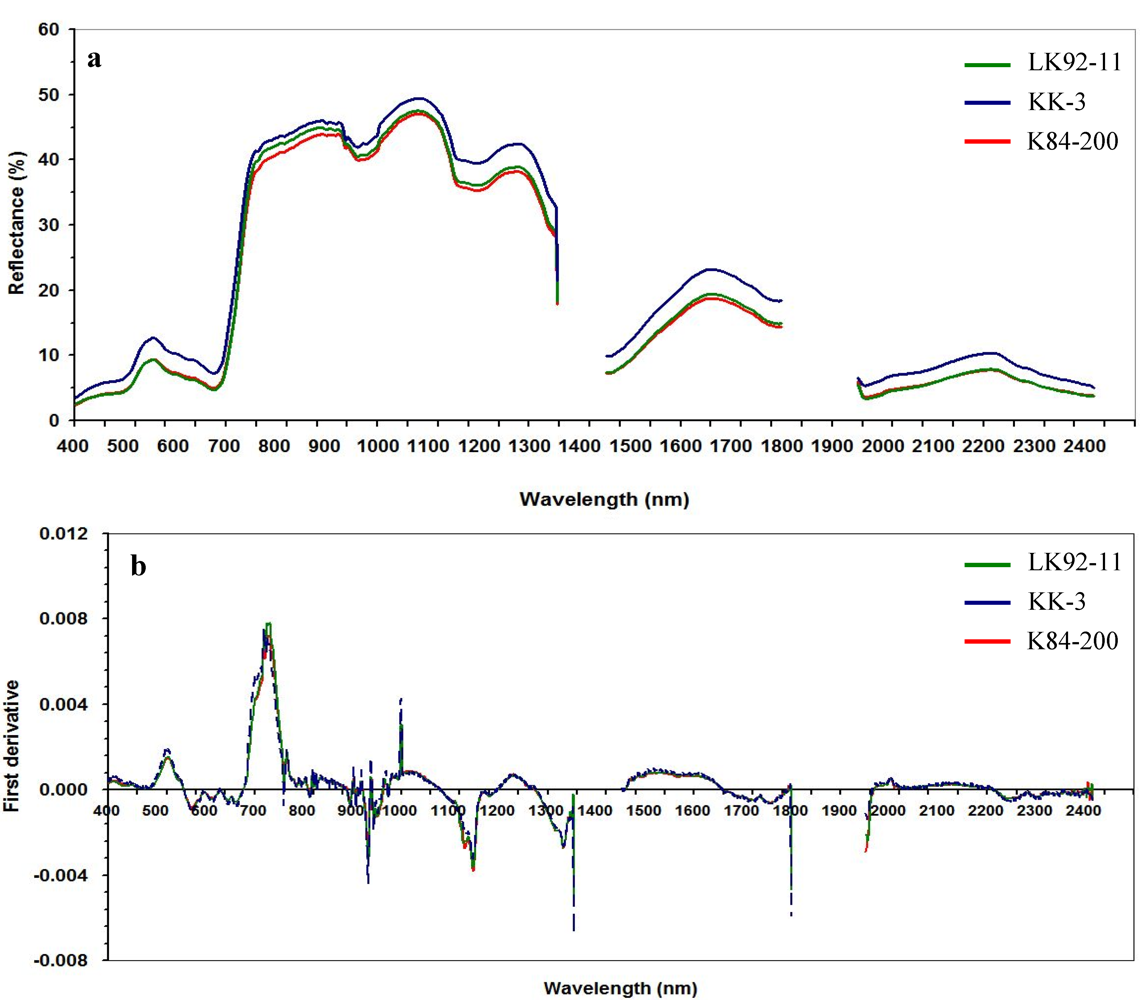
The canopy spectral reflectance values of the three cultivars, shown in Figure 2(a), were averaged. The mean spectra (n = 60) between K84-200 and KK-3 are obviously discriminated, while the difference is subtle between LK92-11 and K84-200. Moreover, the spectral reflectance of the erectophile canopy (K84-200) is lower than that of the planophile canopy (KK-3). The highest variations occur in the near-infrared (650–700 nm) and shortwave-infrared regions, which are mainly absorbed by the water (1,300–1,400 nm). An averaged FDS is illustrated in Figure 2(b). This figure clearly displays the variations in the magnitude and position of the absorption features between the three cultivars.
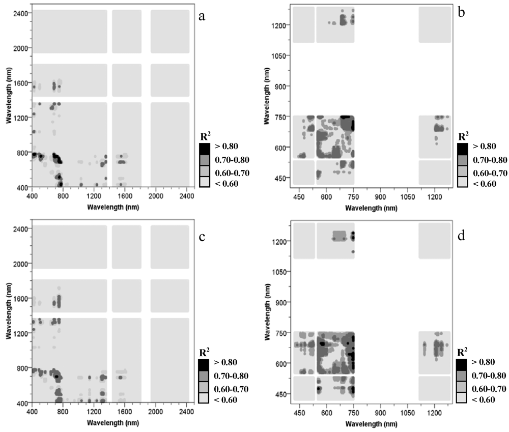
3.2. Relationships between the Nitrogen Concentration and Narrow Vegetation Index
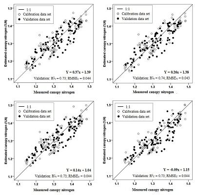
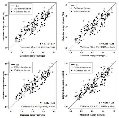
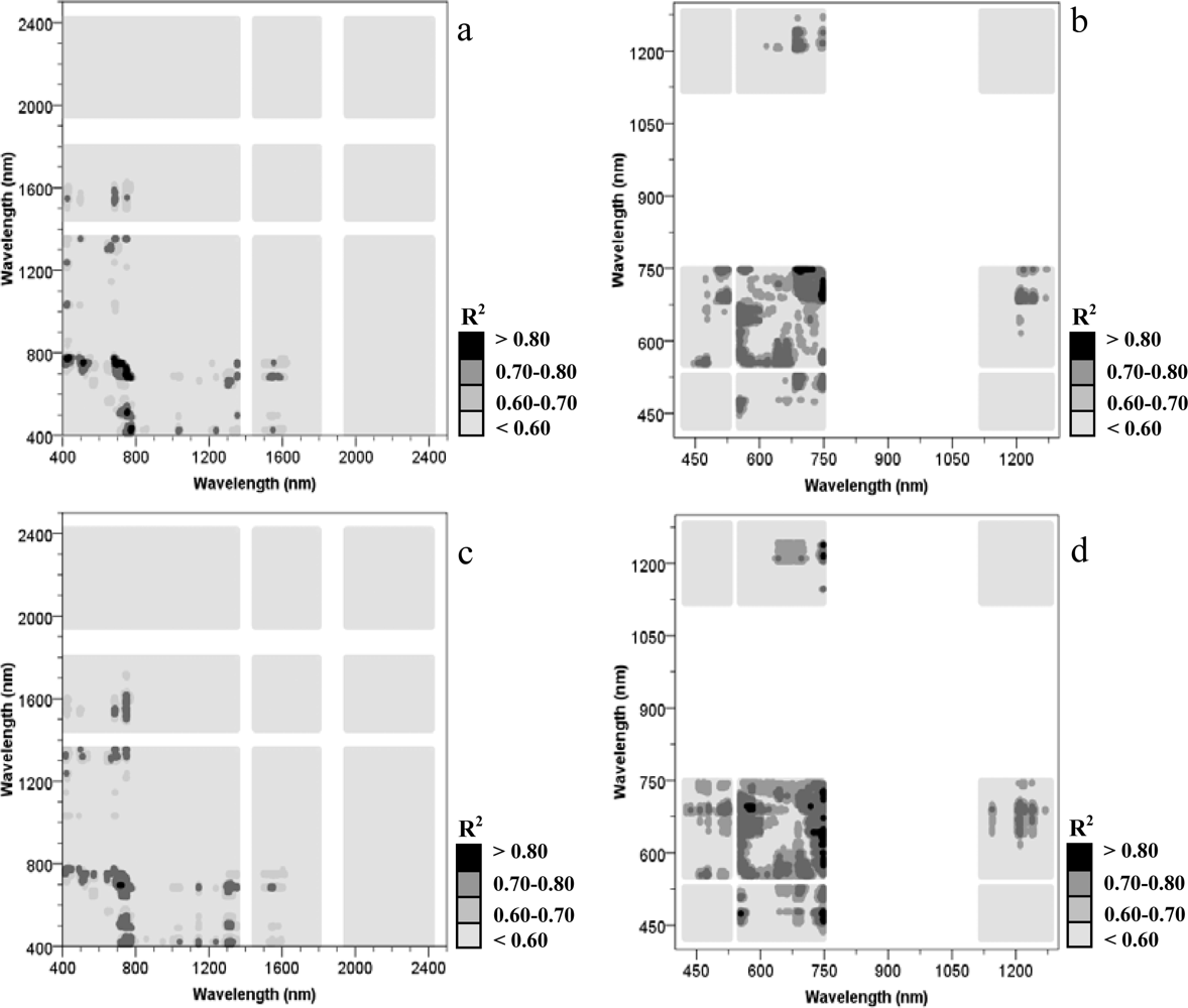
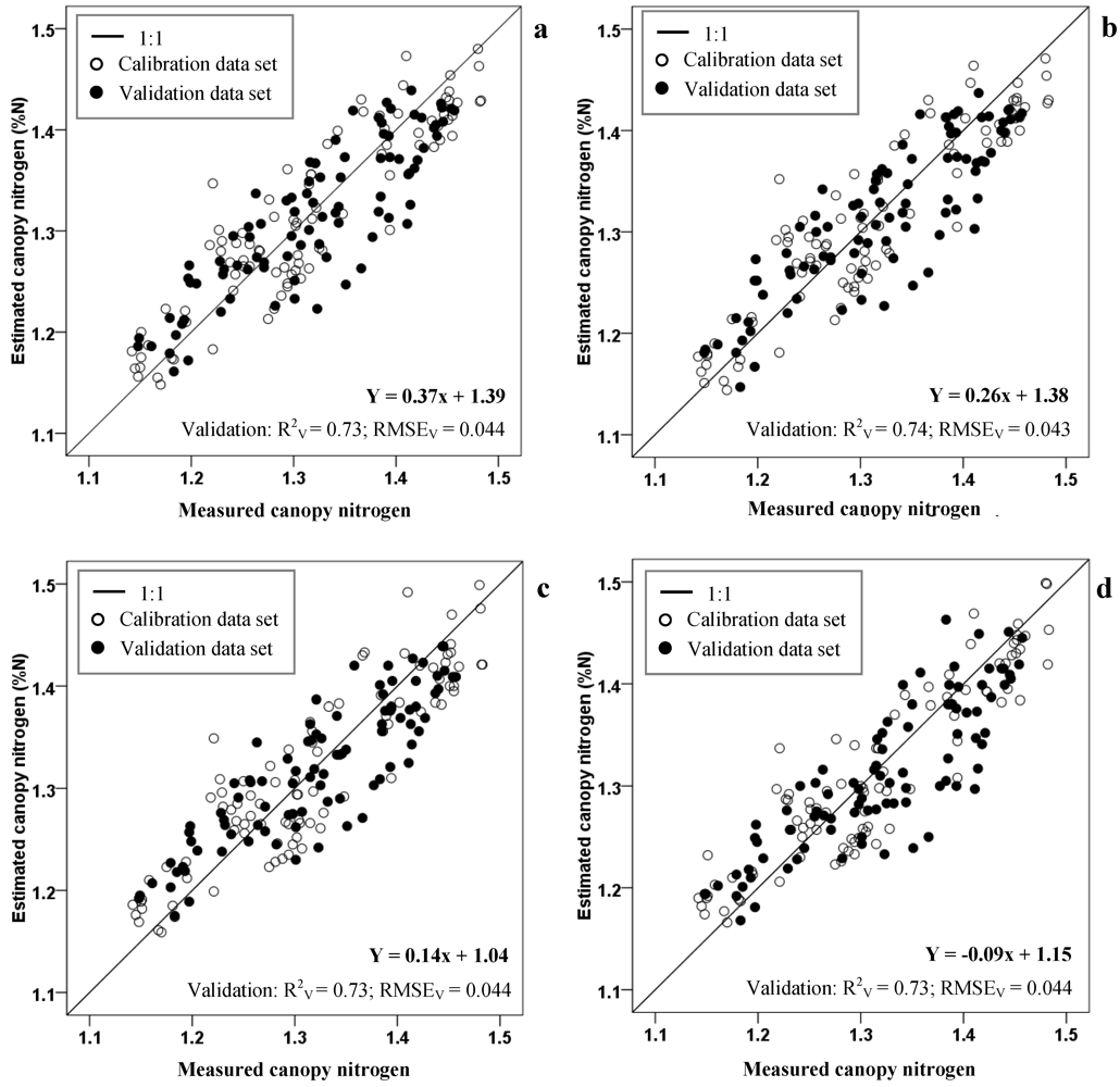
The correlation coefficients between all possible wavelength pairs with R2 ≥ 0.6 are displayed in a correlation plot (Figure 3). The highest correlation regions between the NDI and RVI based on the FDS and the nitrogen concentration were highlighted in the range of 630–750 nm, i.e., the near-infrared and red edge regions. Wavelengths between 675 and 750 nm in the CRDR also constitute the sensitive band for determining the nitrogen status. Table 4 illustrates the model accuracy estimated by the NDI and the RVI, using the combined cultivar data set. The predictive performance of the NDI was slightly higher than that of the RVI. In this experiment, the NDI based on the FDS(750/700) and the RVI based on the FDS(724/700) yielded the highest accuracy, with R2 values of 0.73 and 0.78, RMSEcv values of 0.044 and 0.043% N and RE values of 3.34 and 3.27%N for the validation data set and the pooled data set, respectively. The regression equations are Y = 0.37x + 1.39 and Y = 0.14x + 1.04.
The scatter plots in Figure 4 illustrate the comparison between the measured and estimated nitrogen concentration determined by four models. We found that the region of 510–540 nm and 700–800 nm are the sensitive regions for characterizing the nitrogen status. Table 5 shows the capability of narrow vegetation indices to estimate the nitrogen concentration in sugarcane with the separated cultivars. Partitioning data into the individual cultivars can improve the model precision. The proposed model can mostly explain the nitrogen variation of KK-3, with an accuracy of approximately 90%. Wavelengths between 700 and 750 nm are best suited for predicting nitrogen quality. Selected wavelengths and regression equations are summarized in Table 6.
3.3. Relationships between the Nitrogen Concentration and Spectral Wavelength Determined by a SMLR Technique
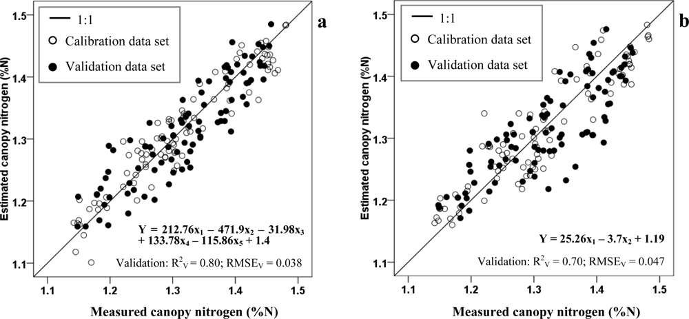
The number of selected spectral wavelengths, used to estimate the nitrogen concentration by SMLR, ranges from two to five. Using the FDS as an independent variable, SMLR selected five sensitive wavelengths, centered at the visible, red edge and far near-infrared regions of the electromagnetic spectrum. The best model yielded R2 values of 0.80 and 0.86, RMSE values of 0.038 and 0.033%N and RE values of 2.88 and 2.50%N validated by an independent data set and a pooled data set, respectively. The regression equation is Y = 212.76x1 – 471.9x2 – 31.98x3 + 133.78x4 – 115.86x5 + 1.4. The selected wavelengths for each data set are summarized in Table 7. The CRDR and BD variables cannot be used to improve the model precision for determining the nitrogen concentration compared with the FDS. Relationships between the measured and estimated nitrogen concentration were determined from the combined and separated cultivar data sets and are depicted in Figure 5(a,b). However, the predictive models developed by a SMLR technique exhibited a higher accuracy than those developed based on the narrow vegetation indices, as indicated by the higher R2 and lower RMSE associated with the former.
Table 8 summarizes the performance of SMLR in estimating the nitrogen concentration of separated cultivars using the different independent variables, including FDS, CRDR and BD. The sensitive wavelengths were shifted from the shortwave to the middle-infrared region. The proposed model can mostly explain the nitrogen variations of KK-3 (94%), LK92-11 (86%) and K84-200 (80%). Partitioning of data into cultivar could increase the estimation capability of the method applied in this research. The selected wavelengths and regression equations used are listed in Table 9.
3.4. Discussion
3.4.1. Utility of the Methods Used in this Study in Estimating the Nitrogen Concentration
Results from this research indicate that field spectroscopy data contains adequate information for determining the nitrogen concentration in sugarcane with combined cultivars. The univariate method has illustrated that the red edge region contains the sensitive wavelengths for explaining the nitrogen variations in sugarcane canopy. This region has been shown to be insensitive to atmospheric and background effects [11], and to be related to chlorophyll [14]. Since, there is a positive strong relationship between nitrogen concentration and chlorophyll [48]. The proposed models using FDS, CRDR and BD as independent variables could explain between 70% and 83% the variation of nitrogen concentration in standing sugarcane canopies. The model RMSE values range from 0.048–0.043%N. The modified estimation model, generated by a SMLR technique using FDS, yields the highest correlation coefficient value of 0.86 and a RMSE value of 0.033 with sugarcane canopy nitrogen concentration. The estimation model developed by SMLR yields a higher correlation coefficient with nitrogen content as compared to the model computed by narrow vegetation indices. This is because the two-wavelength index uses only a limited amount of the spectral information. These results are consistent with those of previous studies [10,33]. In addition, we found that the estimation models developed from the FDS exhibited a higher correlation with the observed nitrogen concentration than those generated from the CRDR and BD. This conclusion agrees with the results of previous studies [26].
3.4.2. Wavelength Selection
The estimation model with the highest predictive accuracy was developed by SMLR technique. The selected wavelengths, including the spectral bands centered at 410, 430, 720, 754 and 1216 nm, were used to predict the nutrient quality in sugarcane. Wavelengths in the visible region (λ = 410 nm and 430 nm), selected for nitrogen concentration estimation, are related to pigment absorption [22]. Several publications have shown a strong correlation between the concentration of nitrogen and chlorophyll a and b [10,22,23,26,43]. Nitrogen is directly related to the photosynthetic process. A strong relationship between chlorophyll absorption bands and nitrogen concentration is therefore expected [10]. Two wavelengths in the shorter region of the red edge (λ = 720 nm) and in the longer region of the red edge (λ = 754 nm), selected by the estimation model, are in agreement with the known nitrogen absorption bands [22]. The wavelength centered at 720 nm is the critical point on the red-edge around which there is the maximum change in the slope of the reflectance spectra per unit. It is also considered as the sensitive band to the temporal variations in crop growth, vegetation stress, and chlorophyll & nitrogen status of plants [42,43,49]. Whereas the wavelength centered at 754 nm is sensitive to the variations of chlorophyll and nitrogen. The last wavelength in the Far Near-Infrared Region (FNIR) (λ = 1,216 nm), is selected as an estimator and is sensitive to plant moisture. The most rapid change falls into the spectra with a change in wavelength in FNIR [50,51]. The wavelength 1,216 nm, which yields the high correlation with the N status, is in disagreement with [26] who found that wavelengths between 1,300–1,350 nm were strongly related to the leaf nitrogen concentration in sugarcane.
3.4.3. Effects of Plant Morphology and Structure on the Spectral Response
The structure of the plant canopy has a significant bearing on its spectral signature [43]. The leaf orientation of the KK-3, K84-200 and LK92-11 cultivar, which were tested in this study, exhibits the planar, erect and mixed structures, respectively. The proposed estimation models in this study could explain most of the nitrogen variations (>90%) in planophile canopy (KK-3). On the other hand, the model precision was quite low in the mixed structures, ∼80–86% (LK92-11), and in the erectophile structure, ∼78–80% (K84-200). Thenkabail et al. [43] concluded that the planophile structure (30 degrees) contributes to a significantly greater reflectance in the near infrared and to a greater absorption in the red when compared with the erectophile structure (65 degree). This summary is consistent with the measured reflectance spectra used in this study, as shown in Figure 2(a). Usually, the Leaf Area Index (LAI) value of planophile structures is higher than that of mixed and erectophiles, which results in the difference of the density of light radiation reaching the mature leaves down the stalk [52]. LAI, therefore, directly influences the spectral profile of sugarcane canopy. In addition, effects from soil brightness on the reflectance spectra of planophile structures are lower than those of other structures. The canopy structure should be taken into consideration when mapping crop nutrient status in rangelands with combined cultivars. This recommendation is consistent with that of the previous study [10].
3.4.4. Performance Comparison of Proposed Models with Previous Models
Most of the previous publications developed models for estimating the nitrogen variations in paddy rice, wheat, cotton or grass, but only in a few cases in sugarcane [26,28]. The previous experiments estimating the nitrogen concentration from hyperspectral data were conducted at the leaf level. In vegetation canopies, near-infrared reflectance is much higher than that for the single leaves. As most of the radiation at near-infrared wavelengths passes through the single leaves, the multiple leaf layers of a canopy have an additive effect on the reflectance [53]. Part of the radiation transmitted by the first leaf layer is reflected back onto subsequent layers [54]. At the canopy level, there are several factors that influence the spectral reflectance, e.g., wind, the solar azimuth angle, light intensity, and canopy architecture [26]. In this paper, the estimation model was developed from the reflectance spectra measured over the sugarcane canopy. Therefore, it is not reasonable to apply the regression equation, published in previous studies, to the data used in this study. Table 10 shows the estimation models to estimate sugarcane nitrogen concentration from field spectroscopy. Based on the results in this study, the performance of the estimation models was more stable and reliable than in previous studies, because of the higher correlation, lower estimation error and the higher number of samples used.
4. Conclusions
The optimal goal of this paper was to develop an estimation model that could explain the nitrogen variations in sugarcane with combined cultivars. Reflectance spectra were measured over the sugarcane canopy. Derivative spectra and absorption features were used as independent variables in univariate and multivariate approaches. The most important conclusions that could be drawn from this study are as follows:
- Stepwise multiple linear regression could explain the nitrogen variations in sugarcane canopy better than a narrow vegetation index. This technique utilizes more than two wavelengths from the entire spectral region (400–2,500 nm) to estimate the dependent variable.
- First Derivative Spectrum (FDS) showed a better relationship with canopy nitrogen concentration than Continuum-Removed Derivative Reflectance (CRDR) and Band Depth (BD) when the models were developed with multivariate approaches and validated with a combined cultivar data set.
- It was concluded that a First Derivative Spectrum (FDS) has potential when used to estimate the nitrogen content in sugarcane with combined cultivars at the maturity stage (9–12 months).
- Visible, red edge and far near-infrared regions contain more information on canopy nitrogen concentration of combined sugarcane cultivars compared to other parts of the electromagnetic spectrum.
- Canopy architecture directly influences the spectral response and the predictive precision. Canopy structure, therefore, should be taken into consideration when mapping sugarcane nutrient quality in rangelands with combined cultivars.
- In the case of a known cultivar, partitioning the data into cultivars could increase the estimation capability of the method applied in this research.
- The modified estimation model, generated by SMLR technique from FDS centered at 410, 426, 720, 754, and 1,216 nm, yields the highest correlation coefficient value of 0.86 and RMSE value of 0.033%N (n = 90) with nitrogen concentration in sugarcane. This result is much better than those of the previous studies.
Overall, since the field spectroscopy data used in this study was measured over the sugarcane canopy under natural atmospheric conditions, the success of field spectroscopy used for estimating nutrient quality in sugarcane allows an additional experiment using the polar orbiting hyperspectral data for the timely determination of crop nutrient status in rangelands without any requirement of the prior cultivar information.
Acknowledgments
This research was supported by the National Center for Genetic Engineering and Biotechnology (BIOTEC), Ministry of Science and Technology, Thailand. We would also like to acknowledge the kind assistance of the ES Research and Development Co. LTD., the Geo-informatics and Space Technology Development Agency (GISTDA) and the Agricultural System and Engineering Laboratory, Asian Institute of Technology. We thank the anonymous reviewers whose comments substantially improved this paper.
References
- Xavier, A.C.; Rudorff, B.F.T.; Shimabukuro, Y.E.; Berka, L.M.S.; Moreira, M.A. Multi-temporal analysis of MODIS data to classify sugarcane crop. Int. J. Remote Sens 2006, 27, 755–768. [Google Scholar]
- Abdel-Rahman, E.M.; Ahmed, F.B. The application of remote sensing techniques to sugarcane (Saccharum spp. hybrid) production: A review of the literature. Int. J. Remote Sens 2008, 29, 3753–3767. [Google Scholar]
- Fageria, N.K. The Use of Nutrients in Crop Plants; Taylor and Francis Group: London, UK, 2009; p. 430. [Google Scholar]
- Thompson, G.D. The Growth of Sugarcane Variety N14 at Pongola, Mount Edgecombe Research Report No. 7; South African Sugar Association Experiment Station: Mount Edgecombe, South Africa, 1991.
- Wiedenfeld, R.P. Effects of irrigation and N fertilizer application on sugarcane yield and quality. Field Crops Res 1995, 43, 101–108. [Google Scholar]
- Spaner, D.; Todd, A.; Navabi, A.; Mckenzie, D.; Goonewardene, L. Cane leaf chlorophyll measures at differing growth stages be used as an indicator of winter wheat and spring barley nitrogen requirements in eastern Canada. J. Agron. Crop. Sci 2005, 91, 393–399. [Google Scholar]
- Roth, G.W.; Fox, R.H.; Marshall, H.G. Plant tissue tests for predicting nitrogen fertilizer requirements of winter Wheat. Agron. J 1989, 81, 50. [Google Scholar]
- Turner, F.T.; Jund, M.F. Assessing the nitrogen requirements of rice crops with a chlorophyll meter. Aust. J. Exp. Agric 1994, 34, 1001–1005. [Google Scholar]
- Wang, S.; Zhu, Y.; Jiang, H.; Cao, W. Positional differences in nitrogen and sugar concentrations of upper leaves relate to plant N status in rice under different N rates. Field Crops Res 2006, 96, 224–234. [Google Scholar]
- Mutanga, O.; Skidmore, A.K.; Prins, H.H.T. Predicting in situ pasture quality in the Kruger National Park, South Africa, using continuum removed absorption features. Remote Sens. Environ 2004, 89, 393–408. [Google Scholar]
- Clevers, J.G.P.W.; Kooistra, L.; Schaepman, M.E. Using spectral information from the NIR water absorption features for the retrieval of canopy water content. Int. J. Appl. Earth Obs. Geoinf 2008, 10, 388–397. [Google Scholar]
- Stroppiana, D.; Boschetti, M.; Brivio, P.A.; Bocchi, S. Plant nitrogen concentration in paddy rice from field canopy hyperspectral radiometry. Field Crops Res 2009, 111, 119–129. [Google Scholar]
- Delegido, J.; Alonso, L.; Gonzalez, G.; Moreno, J. Estimating chlorophyll content of crops from hyperspectral data using a normalized area over reflectance curve (NAOC). Int. J. Appl. Earth Obs. Geoinf 2010, 12, 165–174. [Google Scholar]
- Jain, N.; Ray, S.S.; Sinph, J.P.; Panigrahy, S. Use of hyperspectral data to assess the effects of different nitrogen application on a potato crop. Prec. Agr 2007, 8, 225–239. [Google Scholar]
- Yao, X.; Zhu, Y.; Tian, Y.C.; Feng, W.; Cao, W. Exploring hyperspectral bands and estimation indices for leaf nitrogen accumulation in wheat. Int. J. Appl. Earth Obs. Geoinf 2010, 12, 89–100. [Google Scholar]
- Galvao, L.S.; Formaggio, A.R.; Tisot, D.A. Discrimination of sugarcane varieties in Southeastern Brazil with EO-1 Hyperion data. Remote Sens. Environ 2005, 94, 523–534. [Google Scholar]
- Vaiphasa, C.; Skidmore, A.K.; De Boer, W.F.; Vaiphasa, T. A hyperspectral band selector for plant species discrimination. ISPRS J. Photogramm 2007, 62, 225–235. [Google Scholar]
- Kamal, M.; Phinn, S. Hyperspectral data for mangrove species mapping: A comparison of pixel-based and object-based approach. Remote Sens 2011, 3, 2222–2242. [Google Scholar]
- Apan, A.; Held, A.; Phinn, S.; Markley, J. Detecting sugarcane ‘Orange Rust’ disease using EO-1 hyperion hyperspectral imagery. Int. J. Remote Sens 2004, 25, 489–498. [Google Scholar]
- Liu, Z.; Huang, J.; Tao, R.; Zhou, W.; Zhang, L. Characterizing and estimating fungal disease severity of rice brown spot with hyperspectral reflectance data. Rice Sci 2008, 15, 232–242. [Google Scholar]
- Vigneau, N.; Ecarnot, M.; Rabatel, G.; Roumet, P. Potential of field hyperspectral imaging as a non destructive method to assess leaf nitrogen content in Wheat. Field Crops Res 2011, 122, 25–31. [Google Scholar]
- Kumar, L.; Schmidt, K.; Dury, S.; Skidmore, A. Imaging Spectrometry and Vegetation Science. In Image Spectrometry; van der Meer, F.D., de Jong, S.M., Eds.; Kluwer Academic Publishers: London, UK, 2001; Volume 4, pp. 111–155. [Google Scholar]
- Curran, P.J.; Dungan, J.L.; Peterson, D.L. Estimating the foliar biochemical concentration of leaves with reflectance spectrometry: Testing the Kokaly and Clark methodologies. Remote Sens. Environ 2001, 76, 349–359. [Google Scholar]
- Read, J.J.; Tarpley, L.; Mc Kinion, J.M.; Reddy, K.R. Narrow waveband reflectance ratios for remote estimation of nitrogen status in cotton. J. Environ. Qual 2002, 31, 1442–1452. [Google Scholar]
- Zarco-Tejada, P.J.; Miller, J.R.; Mohammed, G.H.; Noland, T.L.; Sampson, P.H. Vegetation stress detection through chlorophyll a + b estimation and fluorescence effects on hyperspectral imagery. J. Environ. Qual 2002, 31, 1433–1441. [Google Scholar]
- Abdel-Rahman, E.M.; Ahmed, F.B.; Van den berg, M. Estimation of sugarcane leaf nitrogen concentration using in situ spectroscopy. Int. J. Appl. Earth Obs. Geoinf 2010, 12, S52–S57. [Google Scholar]
- Johnson, R.M.; Richard, E.P., Jr. Prediction of sugarcane sucrose content with high resolution, hyperspectral leaf reflectance measurements. Int. Sugar J 2011, 113, 48–55. [Google Scholar]
- Mokhele, A.; Ahmed, F.B. Estimation of leaf nitrogen and silicon using hyperspectral remote sensing. J. Appl. Remote Sens 2010, 4, 1–18. [Google Scholar]
- Begue, A.; Lebourgeois, V.; Bappel, E.; Todoroff, P.; Pellegrino, A.; Baillarin, F.; Siegmund, B. Spatio-temporal variability of sugarcane fields and recommendations for yield forecast using NDVI. Int. J. Remote Sens 2010, 21, 5391–5407. [Google Scholar]
- Roder, A.; Kuemmerle, T.; Hill, J.; Papanastasis, V.P.; Tsiourlis, G.M. Adaptaetion of a grazing gradient concept to heterogeneous Mediterranean rangelands using cost surface modelling. Ecol. Model 2007, 204, 387–398. [Google Scholar]
- ASD. Field Spec Pro spectrometer; Analytical Spectral Devices: Boulder, CO, USA, 1995. [Google Scholar]
- Mutanga, O.; Skidmore, A.K. Narrow band vegetation indices overcome the saturation problem in biomass estimation. Int. J. Remote Sens 2004, 25, 1–16. [Google Scholar]
- Darvishzadeh, R.; Skidmore, A.; Schlerf, M.; Atzberger, C.; Corsi, F.; Cho, M. LAI and chlorophyll estimation for a heterogeneous grassland using hyperspectral measurements. ISPRS J. Photogramm 2008, 63, 409–426. [Google Scholar]
- Muchovej, R.M.; Newman, P.R. Nitrogen fertilization of Sugarcane on sandy soil: Yield and leaf nutrient composition. J. Am. Soc. Sugar Cane Tech 2004, 24, 210–224. [Google Scholar]
- SASRI. Leaf Sampling. Information Sheet. South African Sugarcane Research Institute: Mount Edgecombe, South Africa, 2003. [Google Scholar]
- Muchovej, R.M.; Newman, P.R.; Luo, Y. Sugarcane leaf nutrient concentrations: With or without midribs tissue. J. Plant Nutr 2005, 28, 1271–1286. [Google Scholar]
- FOSS. Kjeltec™ 2200Auto Distillation; FOSS Analytical: Hilleroed, Denmark, 2005. [Google Scholar]
- Dawson, T.P.; Curran, P.J. A new technique for interpolating the reflectance red edge position. Int. J. Remote Sens 1998, 19, 2133–2139. [Google Scholar]
- de Jong, S.M. Imaging spectrometry for monitoring tree damage caused by volcanic activity in the long valley caldera, California. Int. J. Appl. Earth Obs. Geoinf 1998, 1, 1–10. [Google Scholar]
- Mutanga, O.; Skidmore, A.K. Continuum-Removed Absorption Features Estimate Tropical Savanna Grass Quality in situ. Proceedings of 3rd EARSeL Workshop on Imaging Spectroscopy, Hersching, Germany, 13–16 May 2003.
- Kokaly, R.F.; Clark, R.N. Spectroscopic determination of leaf biochemistry using band-depth analysis of absorption features and stepwise multiple linear regression. Remote Sens. Environ 1999, 67, 267–287. [Google Scholar]
- Thenkabail, P.S.; Smith, R.B.; De Pauw, E. Hyperspectral vegetation indices and their relationships with agricultural crop characteristics. Remote Sens. Environ 2000, 71, 158–182. [Google Scholar]
- Thenkabail, P.S.; Smith, R.B.; De Pauw, E. Evaluation of narrowband and broadband vegetation indices for determining optimal hyperspectral wavebands for agricultural crop characterization. Photogramm. Eng. Remote Sensing 2002, 68, 607–621. [Google Scholar]
- Motohka, T.; Nasahara, K.N.; Oguma, H.; Tsuchida, S. Applicability of green-red vegetation index for remote sensing of vegetation phenology. Remote Sens 2010, 2, 2369–2387. [Google Scholar]
- Martin, M.E.; Aber, J.D. Estimation of forest canopy lignin and nitrogen concentration and ecosystem processes by high spectral resolution remote sensing. Ecol. Appl 1997, 7, 431–443. [Google Scholar]
- Serrano, L.; Penuelas, J.; Ustin, S.L. Remote sensing of nitrogen and lignin in Mediterranean vegetation for AVIRIS data: decomposing biochemical from structural signals. Remote Sens. Environ 2002, 81, 355–364. [Google Scholar]
- Yi, Q.X.; Huang, J.F.; Wang, F.M.; Wang, X.Z.; Liu, Z.Y. Monitoring rice nitrogen status using hyperspectral reflectance and artificial neural network. Environ. Sci. Tech 2007, 41, 6770–6775. [Google Scholar]
- Yoder, B.J.; Pettigrew-Crosby, R.E. Predicting nitrogen and chlorophyll content and concentrations from reflectance spectra (400–2500 nm) at the leaf and canopy scale. Remote Sens. Environ 1995, 53, 199–211. [Google Scholar]
- Elvidge, C.D.; Chen, Z. Comparison of broadband and narrow-band red and near-infrared vegetation indices. Remote Sens. Environ 1995, 54, 38–48. [Google Scholar]
- Thenkabail, P.S.; Enclona, E.A.; Ashton, M.S.; van der Meer, V. Accuracy assessments of hyperspectral waveband performance for vegetation analysis applications. Remote Sens. Environ 2004, 91, 354–376. [Google Scholar]
- Thenkabail, P.S.; Enclona, E.A.; Ashton, M.S.; Legg, C.; Jean De Dieu, M. Hyperion, KONOS, ALI, and ETM+ sensors in the study of African rainforests. Remote Sens. Environ 2004, 90, 23–43. [Google Scholar]
- Tejera, N.A.; Rodes, R.; Ortega, E. Comparative analysis of physiological characteristics and yield components in sugarcane cultivars. Field Crops Res 2007, 102, 67–72. [Google Scholar]
- Belward, A.S. Spectral Characteristics of Vegetation, Soil and Water in the Visible, Near-Infrared and Middle-Infrared Wavelengths. In Remote Sensing and Geographical Information Systems for Resource Management in Developing Countries; Belward, A.S., Valenzuela, C.R., Eds.; Kluwer: Dordrecht, The Netherlands, 1991. [Google Scholar]
- Hoffer, R.M. Biological and Physical Considerations in Applying Computer Aided Analysis Techniques to Remote Sensor Data. In Remote Sensing: The Quantitative Approach; Swain, P.H., Davis, S.M., Eds.; McGraw Hill: New York, NY, USA, 1978; pp. 227–289. [Google Scholar]
Figure 1.
The study area in Sakaeo Province, in the eastern region of Thailand.
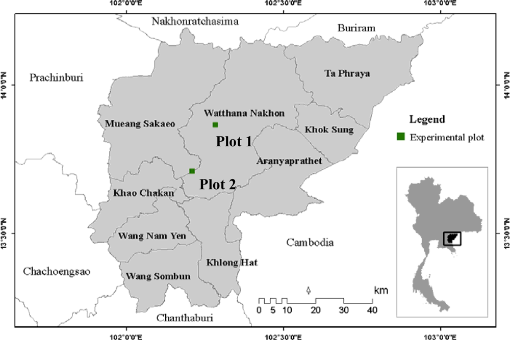
Figure 2.
Comparison of the mean canopy reflectance spectra of sugarcane (N = 60 for each cultivar) between the three different cultivars: (a) original reflectance; and (b) first derivative spectrum.
Figure 2.
Comparison of the mean canopy reflectance spectra of sugarcane (N = 60 for each cultivar) between the three different cultivars: (a) original reflectance; and (b) first derivative spectrum.
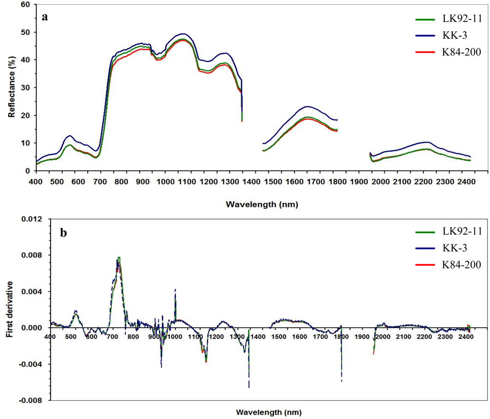
Figure 3.
Contour plots showing the regions with high correlation coefficients (R2 ≥ 0.6) between narrow vegetation index value and nitrogen concentration (n = 90) calculated from all possible combination wavelengths: (a) Normalized Differential Index (NDI) based on First-Derivative Spectrum (FDS); (b) NDI based on Continuum-Removed Derivative Reflectance (CRDR); (c) Ratio Spectral Index (RVI) based on FDS; and (d) RVI based on CRDR.

Figure 4.
Measured versus estimated nitrogen concentration in sugarcane with combined cultivars, using narrow vegetation indices (n = 90): (a) NDI (FDS750, FDS700); (b) NDI (CRDR748, CRDR700); (c) RVI (FDS724, FDS700); and (d) RVI (CRDR748, CRDR630).
Figure 4.
Measured versus estimated nitrogen concentration in sugarcane with combined cultivars, using narrow vegetation indices (n = 90): (a) NDI (FDS750, FDS700); (b) NDI (CRDR748, CRDR700); (c) RVI (FDS724, FDS700); and (d) RVI (CRDR748, CRDR630).
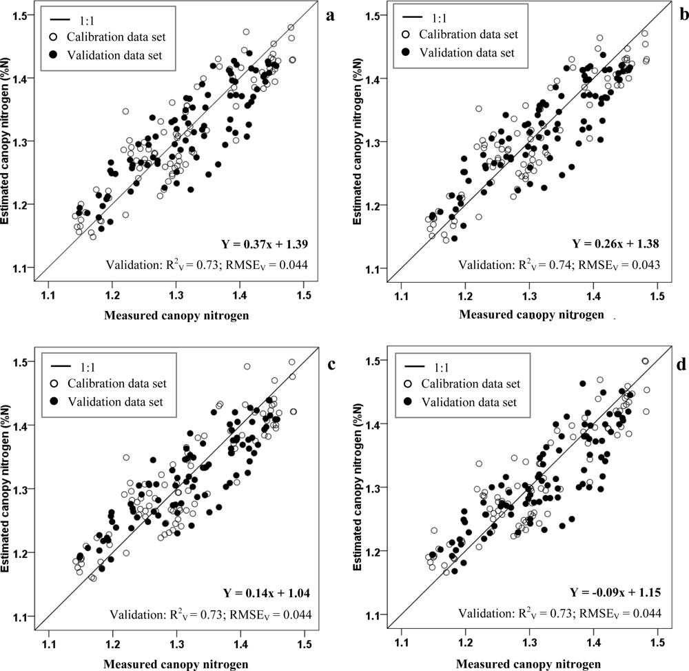
Figure 5.
Measured versus estimated sugarcane nitrogen concentration of combined cultivars; the model was developed by a Stepwise Multiple Linear Regression (SMLR) approach with two independent variables (n = 90): (a) FDS; (b) Band Depth (BD).
Figure 5.
Measured versus estimated sugarcane nitrogen concentration of combined cultivars; the model was developed by a Stepwise Multiple Linear Regression (SMLR) approach with two independent variables (n = 90): (a) FDS; (b) Band Depth (BD).

| Plot 1 | Plot 2 | |
|---|---|---|
| Location | 13.866°N 102.287°E | 13.710°N 102.214°E |
| Soil texture | loamy sand | loamy clay |
| Annual precipitation, mm (2010) | 1,268.2 | 1,296.6 |
| Annual air temperature, °C (2010) | 22.91/35.14 (Min/Max) | 22.8/34.08 (Min/Max) |
| Plot size | 36 m × 76 m | 36 m × 76 m |
Table 2.
Characteristics of the sensor, wavelength covering and spectral resolution used in this study.
| Sensor | Wavelength (nm) | Spectral Resolution (nm) | Number of Bands |
|---|---|---|---|
| Fieldspec® 3 spectroradiometer | 400–1,050 | 1.4 | 465 |
| 1,050–2,500 * | 2 | 560 |
*The spectral regions between 1355–1450 nm, 1800–1950 nm and 2420–2500 nm, which are associated with the water absorption, were excluded from the analysis.
| Data Set | Sample | Min (%N) | Max (%N) | Mean (%N) | Std Deviation (%N) |
|---|---|---|---|---|---|
| Calibration | 90 | 1.142 | 1.483 | 1.313 | 0.098 |
| Validation | 90 | 1.148 | 1.457 | 1.319 | 0.084 |
| Pooled | 180 | 1.142 | 1.483 | 1.316 | 0.091 |
| By Cultivar | |||||
| LK92-11 | 60 | 1.251 | 1.415 | 1.333 | 0.046 |
| KK-3 | 60 | 1.275 | 1.483 | 1.395 | 0.062 |
| K84-200 | 60 | 1.142 | 1.322 | 1.221 | 0.051 |
Table 4.
Performances of narrow vegetation indices calculated from different independent variables for estimating nitrogen concentration in sugarcane with the combined cultivars.
| VI | Variable | λ1/λ2 (nm) | Calibration Data Set (N = 90) | Validation Data Set (N = 90) | Pooled Data Set (N = 180) | |||
|---|---|---|---|---|---|---|---|---|
| R2c | RMSEc | R2v | RMSEv | R2cv | RMSEcv | |||
| NDI | FDS | 750/700 | 0.82 | 0.041 | 0.73 | 0.044 | 0.78 | 0.043 |
| CRDR | 748/690 | 0.82 | 0.041 | 0.73 | 0.043 | 0.78 | 0.043 | |
| BD | 748/680 | 0.81 | 0.042 | 0.70 | 0.047 | 0.76 | 0.045 | |
| RVI | FDS | 724/700 | 0.80 | 0.043 | 0.73 | 0.044 | 0.78 | 0.043 |
| CRDR | 748/630 | 0.83 | 0.041 | 0.73 | 0.044 | 0.78 | 0.043 | |
| BD | 748/670 | 0.82 | 0.042 | 0.70 | 0.048 | 0.76 | 0.045 | |
λ: Selected wavelength in nm; RMSEc, RMSEv and RMSEcv: root mean square error of calibration, validation and relative cross-validation with a 10-fold cross technique, respectively, expressed as %N; R2cv: relative cross-validated coefficient of determination with a 10-fold cross technique; fit between estimated and observed values at the 0.01 level was considered highly significant.
Table 5.
Performances of narrow vegetation indices calculated from different independent variables for estimating nitrogen concentration in sugarcane with the separated cultivar.
| VI | Variable | LK92-11 (N = 60) | KK-3 (N = 60) | K84-200 (N = 60) | ||||||
|---|---|---|---|---|---|---|---|---|---|---|
| λ1 | λ2 | R2v | λ1 | λ2 | R2v | λ1 | λ2 | R2v | ||
| NDI | FDS | 748 | 728 | 0.81 | 718 | 710 | 0.91 | 712 | 706 | 0.80 |
| CRDR | 570 | 748 | 0.80 | 736 | 712 | 0.90 | 712 | 700 | 0.79 | |
| BD | 748 | 584 | 0.78 | 716 | 710 | 0.92 | 746 | 680 | 0.75 | |
| RVI | FDS | 748 | 728 | 0.79 | 718 | 710 | 0.90 | 724 | 692 | 0.82 |
| CRDR | 748 | 510 | 0.78 | 712 | 574 | 0.91 | 712 | 700 | 0.82 | |
| BD | 748 | 586 | 0.78 | 716 | 710 | 0.91 | 712 | 678 | 0.76 | |
λ: Selected wavelength in nm; R2v: root mean square error of calibration, validation; fit between estimated and observed values at the 0.01 level was considered highly significant.
Table 6.
List of regression models developed by the vegetation indices using the different data sets.
| Data set | VI | Variablewavelength | Regression Model | R2v |
|---|---|---|---|---|
| Combined cultivars | NDI | FDS750,700 | Y = 0.37x + 1.39 | 0.73 |
| CRDR748,690 | Y = 0.26x + 1.38 | 0.73 | ||
| BD748,680 | Y = 9.64× + 10.77 | 0.70 | ||
| RVI | FDS724,700 | Y = 0.14x + 1.04 | 0.73 | |
| CRDR748,630 | Y = −0.09x + 1.15 | 0.73 | ||
| BD748,670 | Y = 18.79x + 1.12 | 0.70 | ||
| Separated cultivar - LK92-11 | NDI | FDS748,728 | Y = 0.95x + 1.71 | 0.79 |
| CRDR570,748 | Y = 0.11x + 1.12 | 0.80 | ||
| BD748,584 | Y = 4.58x + 5.72 | 0.78 | ||
| RVI | FDS748,728 | Y = 0.93x + 0.93 | 0.79 | |
| CRDR748,510 | Y = 0.24x + 1.21 | 0.78 | ||
| BD748,586 | Y = 9.05x + 1.14 | 0.78 | ||
| Separated cultivar - KK-3 | NDI | FDS718,710 | Y = 1.59x + 1.09 | 0.91 |
| CRDR736,712 | Y = 0.44x + 1.39 | 0.90 | ||
| BD716,710 | Y = 4.18x + 1.73 | 0.92 | ||
| RVI | FDS718,710 | Y = 0.53x + 0.61 | 0.90 | |
| CRDR712,574 | Y = 0.61x + 2.05 | 0.91 | ||
| BD716,710 | Y = 2.45x – 0.7 | 0.91 | ||
| Separated cultivar - K84-200 | NDI | FDS712,706 | Y = 1.45x + 1.18 | 0.80 |
| CRDR712,700 | Y = 0.75x + 1.23 | 0.79 | ||
| BD746,680 | Y = 3.47x + 4.59 | 0.75 | ||
| RVI | FDS724,692 | Y = 0.08x + 1.07 | 0.82 | |
| CRDR712,700 | Y = 0.39x + 0.84 | 0.82 | ||
| BD712,678 | Y = 0.63x + 0.86 | 0.76 | ||
Table 7.
Performance of stepwise multiple linear regression in estimating the nitrogen concentration in sugarcane with combined cultivar.
| Variable | Wavelength (nm) | Calibration Data set (N = 90) | Validation Data set (N = 90) | Pooled Data Set (N = 180) | |||
|---|---|---|---|---|---|---|---|
| R2c | RMSEc | R2v | RMSEv | R2cv | RMSEcv | ||
| FDS | 410, 430, 720, 754,1216 | 0.90 | 0.030 | 0.80 | 0.038 | 0.86 | 0.033 |
| CRDR | 748, 1158, 1184, 1216, 1276 | 0.89 | 0.033 | 0.64 | 0.053 | 0.78 | 0.043 |
| BD | 748, 1262 | 0.83 | 0.040 | 0.70 | 0.047 | 0.77 | 0.044 |
λ: Selected wavelength in nm; RMSEc, RMSEv and RMSEcv: root mean square error of calibration, validation and relative cross-validation with a 10-fold cross technique, respectively, expressed as %N; R2cv: relative cross-validated coefficient of determination with a 10-fold cross technique; fit between estimated and observed values at the 0.01 level was considered highly significant.
Table 8.
Selected wavelengths and coefficients of determination between the observed nitrogen concentration and the spectral reflectance of separated cultivar.
| Variable | LK92-11 (N = 60) | KK-3 (N = 60) | K84-200 (N = 60) | |||
|---|---|---|---|---|---|---|
| Wavelength (nm) | R2cv | Wavelength (nm) | R2cv | Wavelength (nm) | R2cv | |
| FDS | 670, 754, 1,266, 1,494, 2,313 | 0.86 | 750, 1,104, 1,572, 1,586, 2,153 | 0.93 | 552, 1,032, 1,284, 1,604, 2,359 | 0.80 |
| CRDR | 656, 704, 1,266 | 0.79 | 598, 674, 740, 1,228 | 0.92 | 678, 746, 1,128 | 0.80 |
| BD | 684, 748, 1,228 | 0.82 | 552, 736 | 0.92 | 746 | 0.78 |
R2cv: relative cross-validated coefficient of determination with a 10-fold cross technique; fit between estimated and observed values at the 0.01 level was considered highly significant.
| Data set | Variable | Regression Model | R2v |
|---|---|---|---|
| Combined cultivars | FDS | Y = 212.76x1 – 471.9x2 – 31.98x3 + 133.78x 4 – 115.86x5 + 1.4 | 0.80 |
| CRDR | Y = 55.77x1 + 19.0x2 + 61.92x3 – 73.5x 4 – 34.25x5 + 1.26 | 0.64 | |
| BD | Y = 25.26x1 – 3.7x2 + 1.19 | 0.70 | |
| Separated cultivar -LK92-11 | FDS | Y = 520.59x1 + 14.794x2 – 97.004x3 + 95.08x 4 – 63.49x5 + 1.347 | 0.86 |
| CRDR | Y = 33.04x1 – 18.84x2 – 32.51x3 + 1.72 | 0.79 | |
| BD | Y = −0.47x1 + 17.86x2 – 0.7845x3 + 1.62 | 0.82 | |
| Separated cultivar-KK-3 | FDS | Y = 67.4x1 – 24.64x2 – 136.2x3 – 168.34x4 – 42.007x 5 + 1.4153 | 0.93 |
| CRDR | Y = −14.27x1 – 105.25x2 + 23.31x3 + 8.84x4 + 1.004 | 0.92 | |
| BD | Y = −3.31x1 + 2.26x2 + 1.17 | 0.92 | |
| Separated cultivar - K84-200 | FDS | Y = −194.8x1 + 138.92x2 – 94.52x3 – 213.97x 4 – 22.31x5 + 1.29 | 0.80 |
| CRDR | Y = −64.57x1 + 25.36x2 + 6.34x3 + 28.04x4 + 1.08 | 0.80 | |
| BD | Y = 7.86x1 + 1.12 | 0.78 | |
Table 10.
The estimation models for estimating nitrogen concentration in sugarcane from field spectroscopy compared with previous publications (unit: % nitrogen).
| Spectral Parameter | Regression Equation | Validation | No. of Samples | Study Level | Reference | |
|---|---|---|---|---|---|---|
| R2 | RMSE | |||||
| RVI (FDS741, FDS1323) | Y = −0.237x + 0.587 | 0.74 | 0.084 | 25 | Leaf | [26] |
| RVI (R740, R720) | Y = 0.73x + 0.753 | 0.81 | 0.103 | 37 | Leaf | [28] |
| NDI (FDS750, FDS700) | Y = 0.37x + 1.39 | 0.78 | 0.043 | 90 | Canopy | This paper |
| RVI (FDS724, FDS700) | Y = 0.14x + 1.04 | 0.78 | 0.043 | 90 | Canopy | This paper |
| FDS (410, 430, 720, 754,1216) * | Y = 212.76x1 – 471.9x2 – 31.98x3 + 133.78x 4 – 115.86x5 + 1.4 | 0.86 | 0.033 | 90 | Canopy | This paper |
*developed by SMLR technique.
Share and Cite
MDPI and ACS Style
Miphokasap, P.; Honda, K.; Vaiphasa, C.; Souris, M.; Nagai, M. Estimating Canopy Nitrogen Concentration in Sugarcane Using Field Imaging Spectroscopy. Remote Sens. 2012, 4, 1651-1670. https://doi.org/10.3390/rs4061651
AMA Style
Miphokasap P, Honda K, Vaiphasa C, Souris M, Nagai M. Estimating Canopy Nitrogen Concentration in Sugarcane Using Field Imaging Spectroscopy. Remote Sensing. 2012; 4(6):1651-1670. https://doi.org/10.3390/rs4061651
Chicago/Turabian StyleMiphokasap, Poonsak, Kiyoshi Honda, Chaichoke Vaiphasa, Marc Souris, and Masahiko Nagai. 2012. "Estimating Canopy Nitrogen Concentration in Sugarcane Using Field Imaging Spectroscopy" Remote Sensing 4, no. 6: 1651-1670. https://doi.org/10.3390/rs4061651