The polarimetric synthetic aperture radar (PolSAR) data have never been so widely available to the remote sensing community as it is today, thanks to the launch of recent systems such as ALOS-PALSAR, RADARSAT-2, TerraSAR-X, etc. Effective and efficient interpretation of such mass amount of data thus meets its urgent need. Among the many analyzing tools, polarimetric scattering power decomposition methods [1–9] have become a popular choice because of their clear physical explanation, convenient implementation, and easy visual interpretation.

The original three-component decomposition proposed by Freeman and Durden [1] models the volume scattering as a cloud of uniformed distributed dipoles, and this leads to the use of a fixed coherency matrix. However, a practical issue associated with a fixed volume scattering model is that negative powers which are physically unacceptable may arise for the extracted surface and double-bounce scattering. Attempts have been made to correct such a problem as in [2,3]. In a more recent paper, a non-negative eigen-value constraint has been added [4]. The volume scattering power is obtained as the maximum value retaining the positive-definiteness of the remaining covariance matrix. The surface scattering and double-bounce scattering powers are thus derived through eigen-decomposition. Such treatment also produces a fourth component, called the remainder, which may not necessarily represent any known scattering mechanism. Arii et al. [5] take a further step in this framework by introducing an adaptive volume scattering model. The adaptive parameters are determined by minimizing the power in the covariance matrix after the volume scattering is subtracted. This method generally takes longer to process because numerical searching in the parameter space is needed.

In this paper, we modify the three-component scattering power decomposition method with an adaptive volume scattering model. The adaptive volume scattering model is proposed with three purposes. Firstly, it is to render a mathematically rigorous treatment for eliminating negative powers; secondly, it will not drastically deviate from existing physically-based models (e.g., cloud of dipoles) in vegetated areas; last, it remains easy and fast given the large dimensions of remotely sensed data. The paper is organized as follows. In Section 2, double transformation of the coherency matrix is introduced as a preprocessing step. In Section 3, the adaptive volume model is proposed together with the associated decomposition algorithm. In Section 4, experimental results with PolSAR data are presented. Finally Section 5 gives some discussion and concludes the paper.

In this section, we adopt the method of [6] to perform a double transformation on the coherency matrix as a preprocessing of the PolSAR data. It has been shown that this procedure helps discriminate oblique urban areas from vegetation and consequently gives a more accurate result [3,6,7]. In the following, we describe the transformation method in order to be self-contained. Some important properties of the transformed coherency matrix are also pointed out which accounts for the success of the proposed decomposition as will be explained in Section 4.

The volume scattering is originally modeled by a cloud of uniformly distributed dipoles [1] whose coherency matrix is given by: (11) T V = [ 2 0 0 0 1 0 0 0 1 ] .

However, it has been observed that this model sometimes leads to over-estimation of the volume scattering power and consequently generates a negative power in the derived surface and double-bounce scattering [3]. This phenomenon happens whenever T′₁₁ < 2T′₃₃ in the transformed coherency matrix. In order to prevent such a problem, we relax the volume scattering model as follows: (12) T V ( γ ) = [ γ 0 0 0 1 0 0 0 1 ] , 0 ≤ γ ≤ 2 .

Equation (12) is able to represent a range of existing volume scattering models by introducing the adaptive parameter γ. For example, when γ = 2, then it denotes a cloud of dipoles [1]; when γ = 1, then it is the maximum randomness model proposed by An et al. [3]; when γ = 0, it becomes the extended volume scattering model for urban areas [9] (except for a different scatterer orientation distribution).

The parameter γ can be adaptively determined by choosing the best fit of the volume scattering to the observed data. Specifically, we employ the concept of a similarity parameter proposed in [10]. Mathematically the optimization problem is modeled as: (13) γ * = arg max 0 ≤ γ ≤ 2 { | 〈 T ′ , T V ( γ ) 〉 | ‖ T ′ ‖ ‖ T V ( γ ) ‖ } .

The reason why the similarity parameter is chosen is that it offers the most natural way to compare two matrices. In fact, it represents the inner product of the vector space spanned by 3 × 3 Hermitian matrices. If we define the inner product of two Hermitian matrices A and B as Tr(A^HB) where Tr(.) denotes the trace, then it is easy to derive the solution of Equation (13) as follows: (14a) T 11 ′ < T 22 ′ + T 33 ′ ⇒ γ * = 2 T 11 ′ T 22 ′ + T 33 ′ , (14b) T 11 ′ > T 22 ′ + T 33 ′ ⇒ γ * = 2 .After γ^* has been determined, the remaining procedure is the same to that of the Freeman-Durden decomposition [1]. However, it can be shown that as a consequence of the adaptive volume model Equation (14), the negative power problem will be completely avoided. After subtracting the volume scattering from T′, the remaining coherency matrix becomes: (15) T SD = T ′ − T 33 ′ T V ( γ * ) = [ T 11 ′ − γ * T 33 ′ T 12 ′ 0 ( T 12 ′ ) * T 22 ′ − T 33 ′ 0 0 0 0 ] .Note, in Equation (15) T′₂₂ − T′₃₃ always holds as a result of the double transformation introduced in Section 2. It is also easy to verify that T′₁₁ − γ^*T′₃₃ > 0 as a result of Equation (14). In other words, both diagonal elements remain positive, which prevents any possible negative solutions.

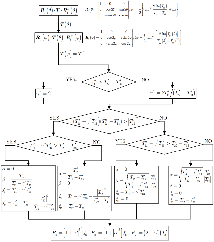
Still, positivity in the diagonal elements does not always guarantee a solution when equating the remaining coherency matrix to the weighted sum of surface and double-bounce models, that is: (16) T SD = f S T S + f D T D = f S [ 1 β 0 β * | β | 2 0 0 0 0 ] + f D [ | α | 2 α 0 α * 1 0 0 0 0 ] , | α | < 1 , | β | < 1 ,where f_S, f_D, α, and β are unknowns to be determined. According to Equations (15) and (16), one needs to solve the following equations: (17a) f S + f D | α | 2 = T 11 ′ − γ * T 33 ′ , (17b) f S | β | 2 + f D = T 22 ′ − T 33 ′ , (17c) f S β + f D α = T 12 ′ .

Whether a solution exists to Equation (17) depends on the relationship between (T′₁₁ − γ^*T′₃₃) (T′₁₁ − T′₃₃) and |T′₁₂|². If (T′₁₁ − γ^*T′₃₃)(T′₁₁ − T′₃₃) ≥ |T′₁₂|², then at least one physically meaningful (non-negative power) solution exists to Equation (17). In fact, the common treatment by assuming there is a dominant scattering mechanism [1] gives one a reasonable result. Another solution can be also derived by the eigen-decomposition approach [4].

However, if (T′₁₁ − γ^*T′₃₃)(T′₁₁ − T′₃₃) < |T′₁₂|², it can be proved that no solution to Equation (17) exists (Appendix 1). In this case f_S, f_D, α, and β and are found by: (18) min f S , f D , α , β { | f S β + f D α − T 12 ′ | } subject   to : f S + f D | α | 2 = T 11 ′ − γ * T 33 ′ , f S | β | 2 + f D = T 22 ′ − T 33 ′ .The solution of the above problem is as follows (Appendix 1): (19a) T 11 ′ − γ * T 33 ′ > T 22 ′ − T 33 ′ ⇒ f S = T 11 ′ − γ * T 33 ′ , f D = 0 , β = T 22 ′ − T 33 ′ T 11 ′ − γ * T 33 ′ T 12 ′ | T 12 ′ | , (19b) T 11 ′ − γ * T 33 ′ < T 22 ′ − T 33 ′ ⇒ f S = 0 , f D = T 22 ′ − T 33 ′ , β = T 11 ′ − γ * T 33 ′ T 22 ′ − T 33 ′ T 12 ′ | T 12 ′ | .Note that in Equation (19a) the value of α has no significance because the double-bounce scattering does not contribute to the total power (f_D = 0) and vice versa.

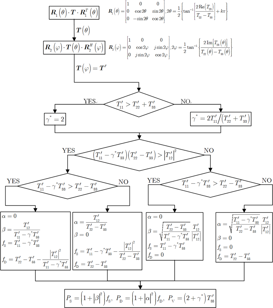
To sum up, the entire procedure for decomposing the PolSAR data using the adaptive volume scattering models is illustrated by the flowchart in Figure 1.

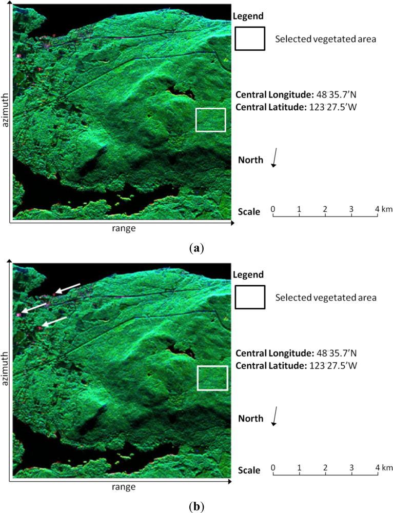
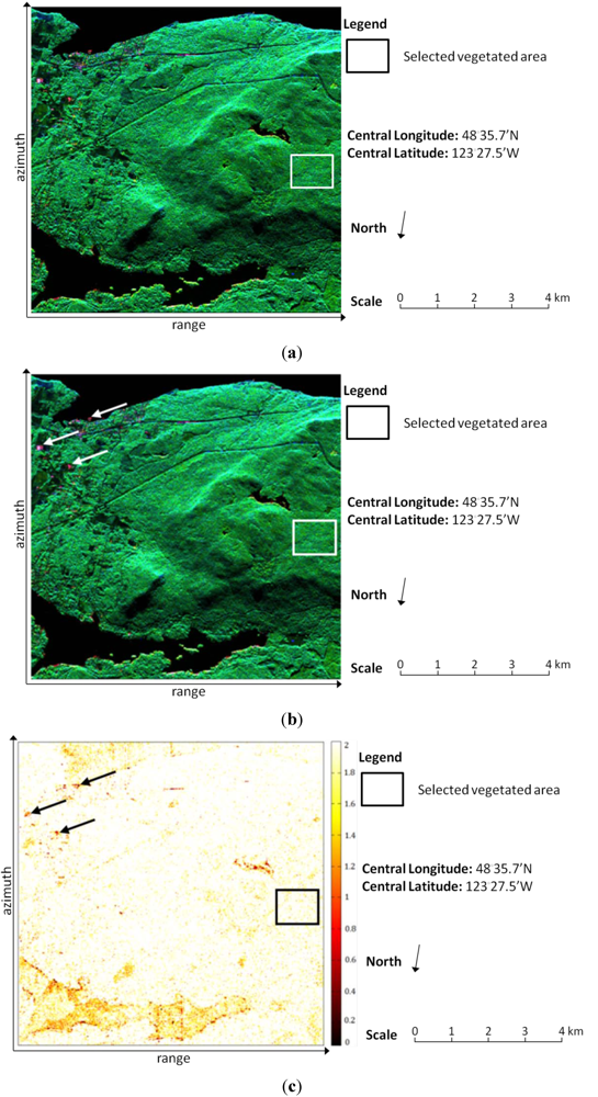
A C-band PolSAR image acquired by the NASA/JPL (National Aeronautics and Space Administration/Jet Propulsion Laboratory) Airborne SAR (AIRSAR) is selected for testing the proposed method. The image is originally multi-look processed but further spatial multi-looking is performed by combining 2 × 2 (range × azimuth) neighboring pixels in order to suppress the speckle effect. The image scene is primarily covered by forested areas which can be used for validating the volume scattering model. 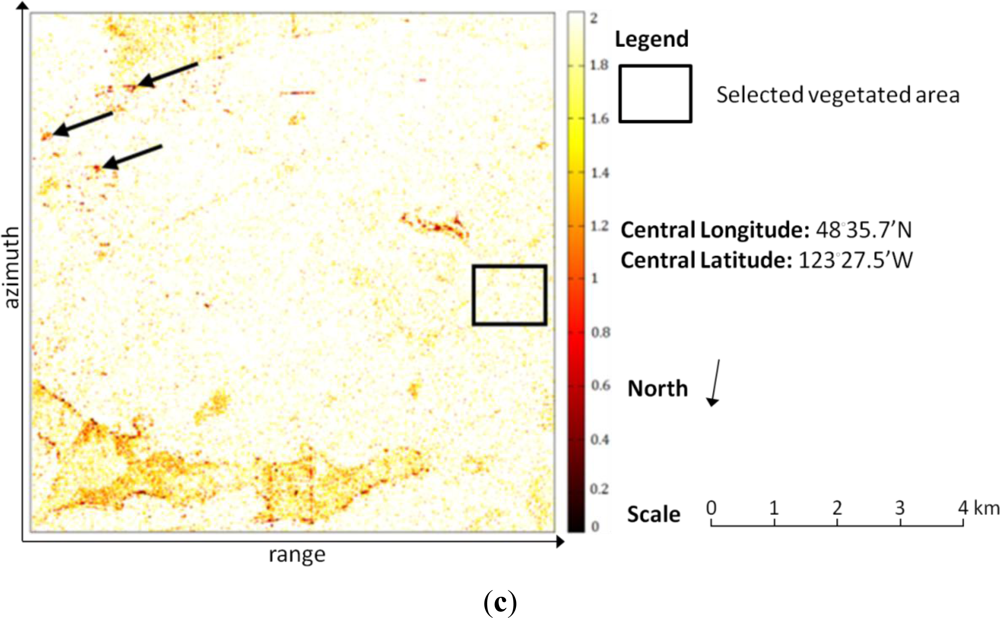Figure 2(a) displays the color-coded decomposition image with a fixed volume scattering model of Equation (11) and Figure 2(b) is the color-coded decomposition image with the adaptive volume scattering model of (12). Furthermore, Figure 2(c) shows the map of γ in the adaptive volume scattering model for each pixel. It can be seen that in most of the forested area, γ is equal or near to the theoretical value of 2. For example, the averaged volume scattering model within the selected rectangle in Figure 2(c) is: (20) T ¯ V ≈ [ 1.95 0 0 0 1 0 0 0 1 ] .

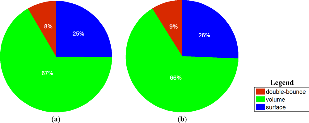
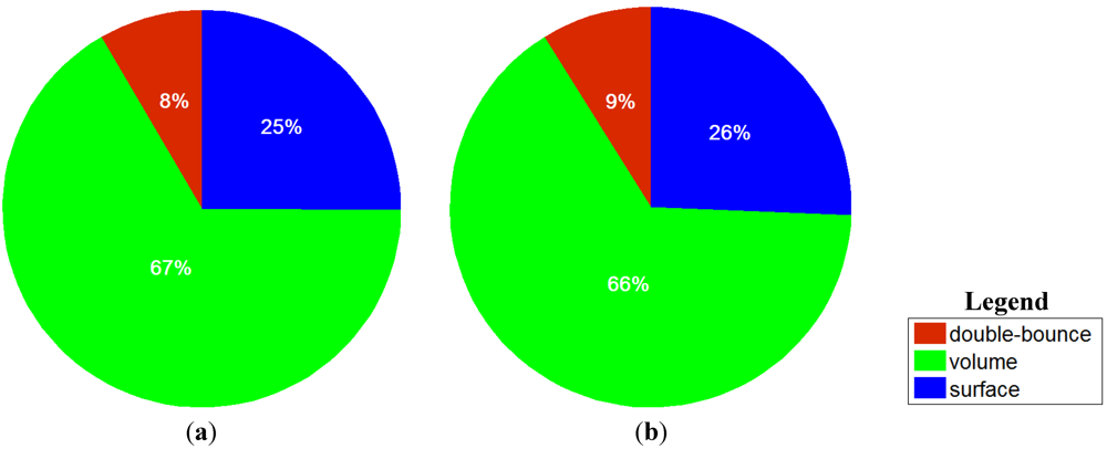
This is very close to the original model of Equation (11) which prevents volume scattering from being under-estimated in vegetated areas. In order to examine the results quantitatively, the power distributions of Figure 2(a,b) in the same selected patches are shown in Figure 3. It can be seen that in the vegetated area, using the fixed volume scattering model and the adaptive scattering model produce very similar results. However, for man-made structures, as indicated by the arrows in Figure 2, γ is much lower than 2, indicating the volume scattering is significantly reduced so that the surface and double-bounce scattering are enhanced. Moreover, while the decomposition result with the fixed volume scattering model produces negative powers for 18,965 pixels out of a total of 327,168 pixels, the proposed method gives positive solutions all over the image.

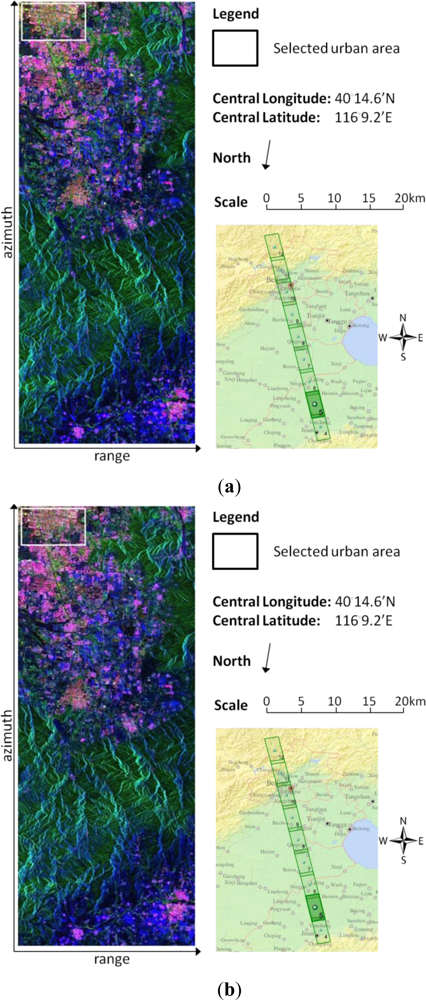
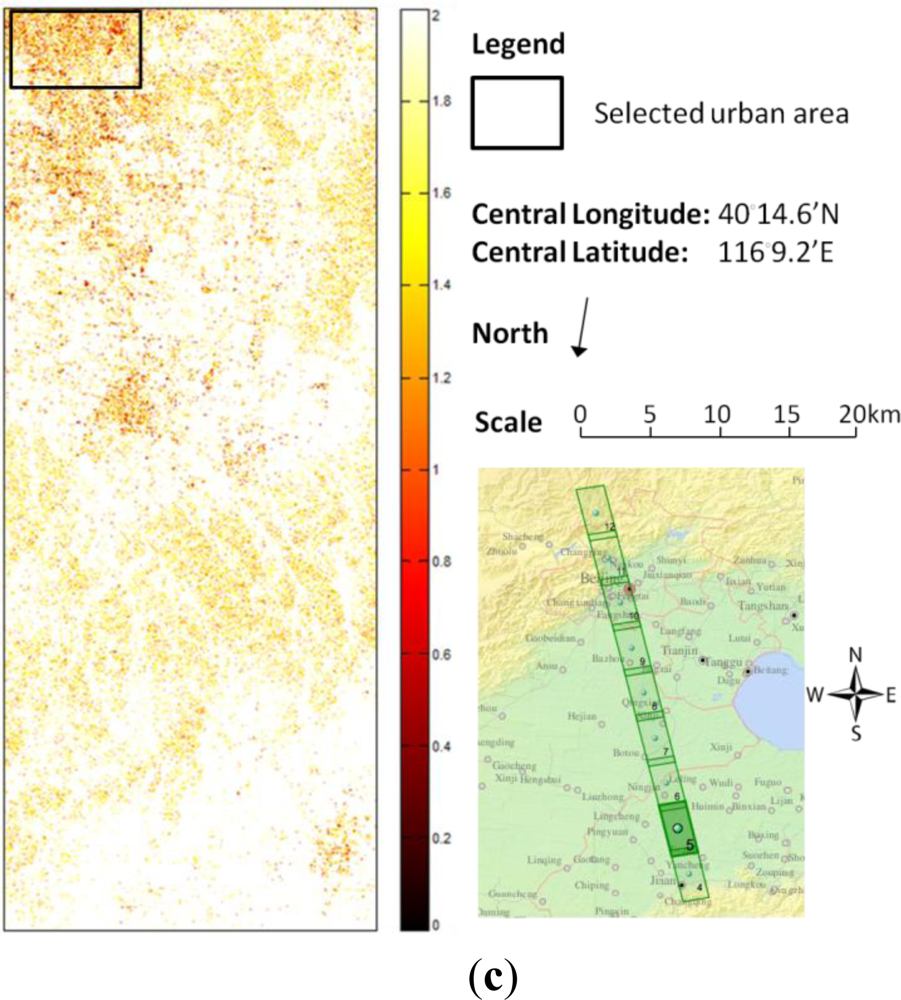
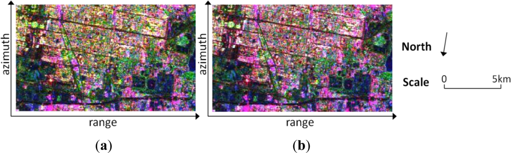
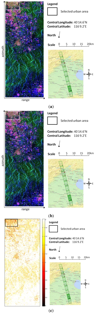
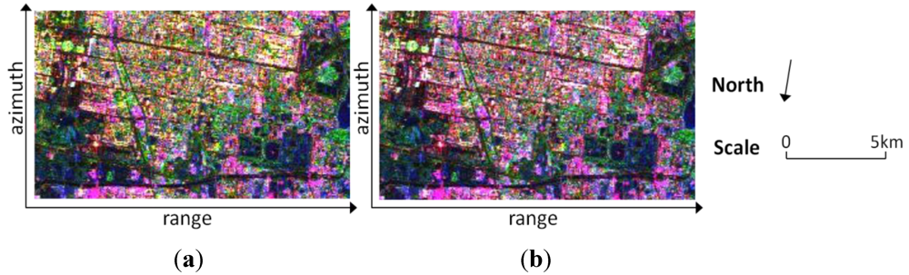
The ability of the proposed method to improve discrimination of man-made structures is more evident in Figure 4, where a PolSAR image acquired by ALOS-PALSAR over the Beijing suburban area is experimented with. Spatial multi-looking has been performed by combining 12 (azimuth)× 2 (range) pixels so that square ground spacing is approximately achieved. Again, it can be seen from Figure 4(c) that in the urban area, the parameter (and consequently the volume scattering power) is significantly reduced. 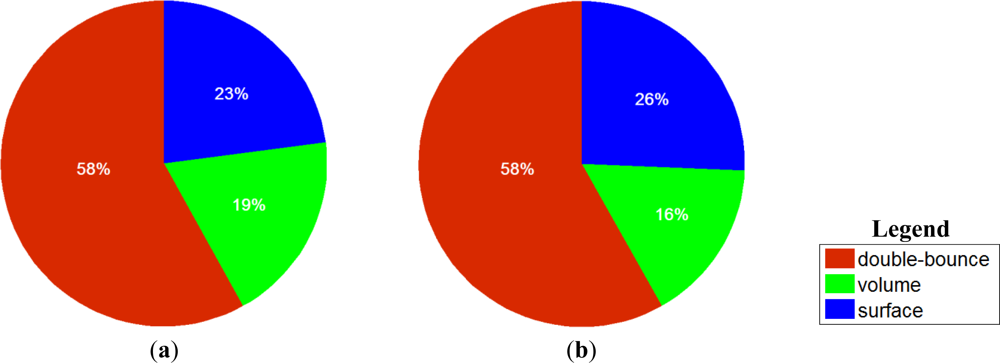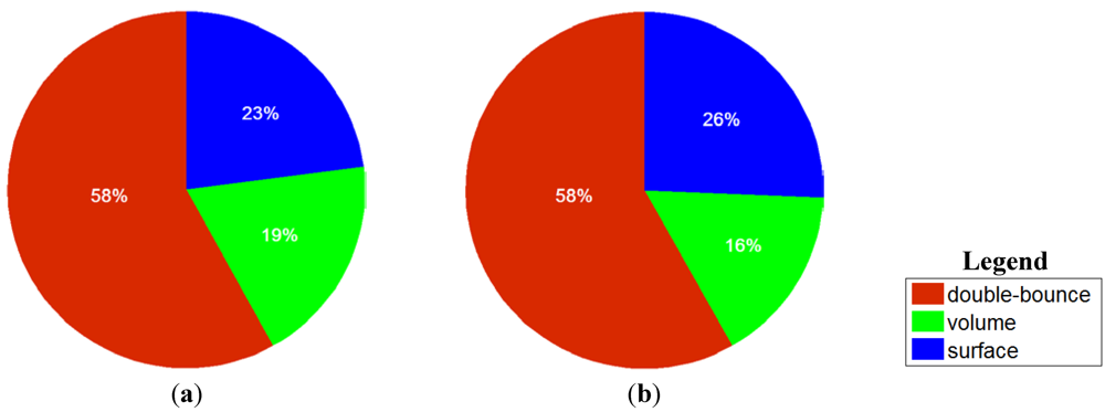This phenomenon can be also observed in the upper right corners of both Figure 4(a,b) which are correspondingly zoomed in Figure 5(a,b). Again, we draw the power distributions for the selected urban area and the results are shown in Figure 6. Compared to Figure 3, we can see that the volume scattering power is more suppressed in the urban area than in the vegetated area by the proposed method. This helps to discriminate manmade structures especially oblique to the radar azimuth direction as in Figure 5.

It is worth noting that the adaptive volume scattering model proposed in this paper is similar to that used by Freeman [11], which can be rewritten in its equivalent coherency matrix form as: (21) T ˜ V ( γ ) = [ γ 0 0 0 1 0 0 0 1 ] , 1 ≤ γ ≤ ∞By comparing Equations (12) and (21), the difference lies in the range for γ. However, Equation (21) cannot be directly used in the three-component decomposition scheme because there exists risk in over-estimating the volume scattering power (note γ can be arbitrarily large by definition). Instead, Freeman proposed to use it in a two-component scattering model for fitting the PolSAR data from forests. In our model, on the other hand, we specifically restrict the upper bound of γ. This is validated by Equation (20) where the averaged volume scattering model in forested areas indeed approximates the maximum theoretical setting. In addition, our model tries to account for the volume scattering mechanism in urban areas by letting γ < 1, which equivalently indicates that the HH-VV correlation is out of phase, i.e., Re(S_HH S VV *) < 0. An explanation of this phenomenon is that the volume scattering within urban areas can be affected by randomly orientated double-bounce scatterers. Our experiments showed that discrimination of urban areas is improved by such an assumption.

In this paper, we have proposed an adaptive three-component power decomposition method for PolSAR data. This method modifies the original Freeman-Durden decomposition [1] by adopting an adaptive volume scattering model. Although our adaptive model takes a similar form to that in [11], there exist significant distinctions including the range of the adaptive parameter as well as the decomposition methodology. In [11], the adaptive volume scattering model is fitted under a two-component decomposition scheme where the adaptive parameter is derived by solving established equations; while in our method the adaptive parameter is derived by solving an optimization problem thanks to the use of a similarity parameter [10]. This treatment enables us to incorporate the adaptive volume scattering model into the three-component decomposition scheme and the increased methodological complexity is negligible.

Experimental results demonstrate that, compared with the original Freeman-Durden decomposition with the fixed volume scattering model, the proposed method produces similar/better decomposition results in vegetated areas, but on the other hand is able to improve discrimination in urban regions. In addition, the proposed method always produces non-negative powers and the power sum of all components equals the total power. This is done with mathematical rigor rather than in an ad-hoc fashion so that further quantitative analysis can be reliably conducted based on the decomposition result.