Development of a UAV-LiDAR System with Application to Forest Inventory


Abstract
:
1. Introduction
1.1. Background
1.2. Objectives
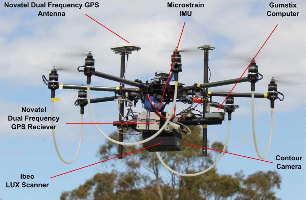
2. Hardware
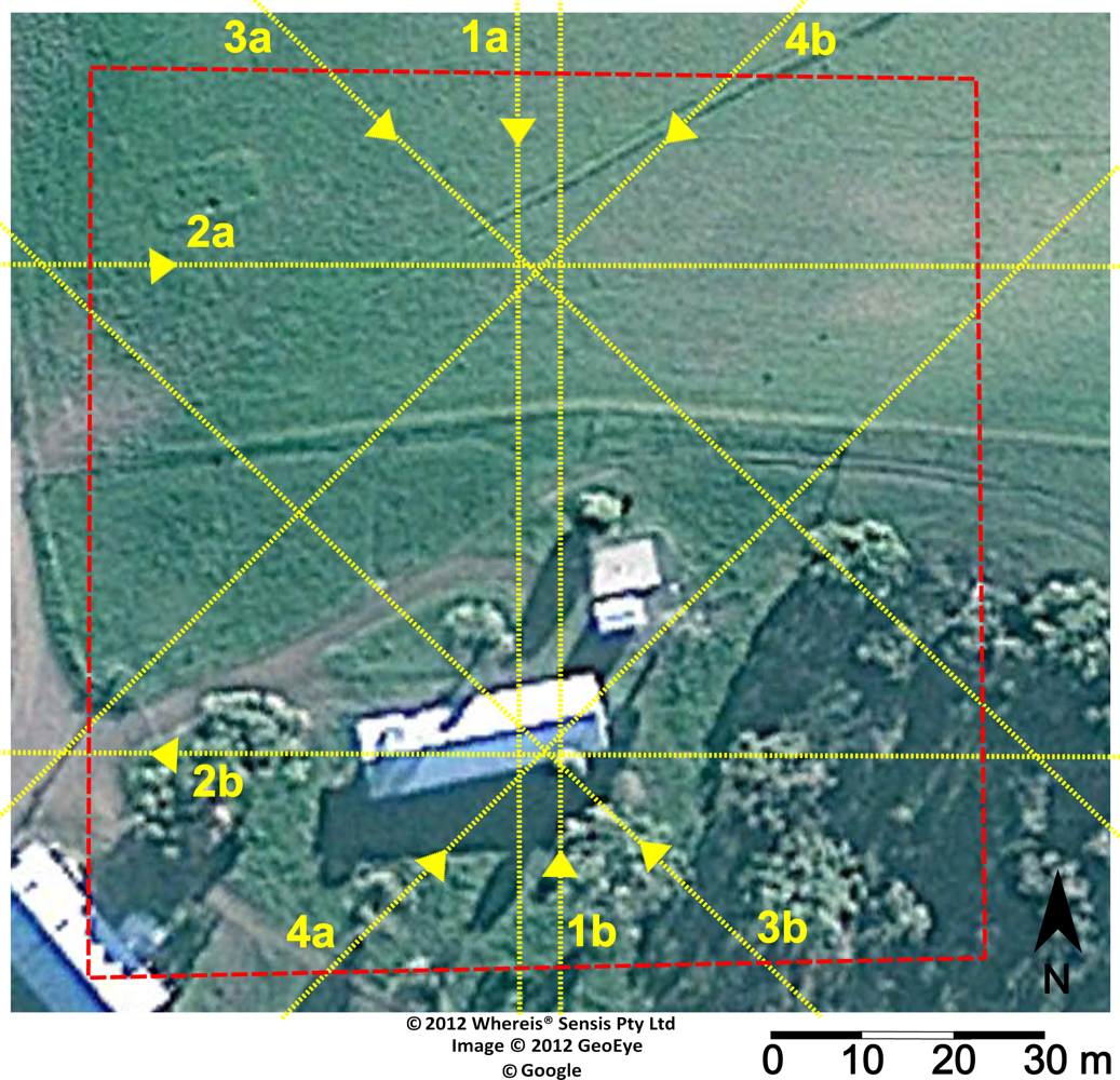
3. Methodology
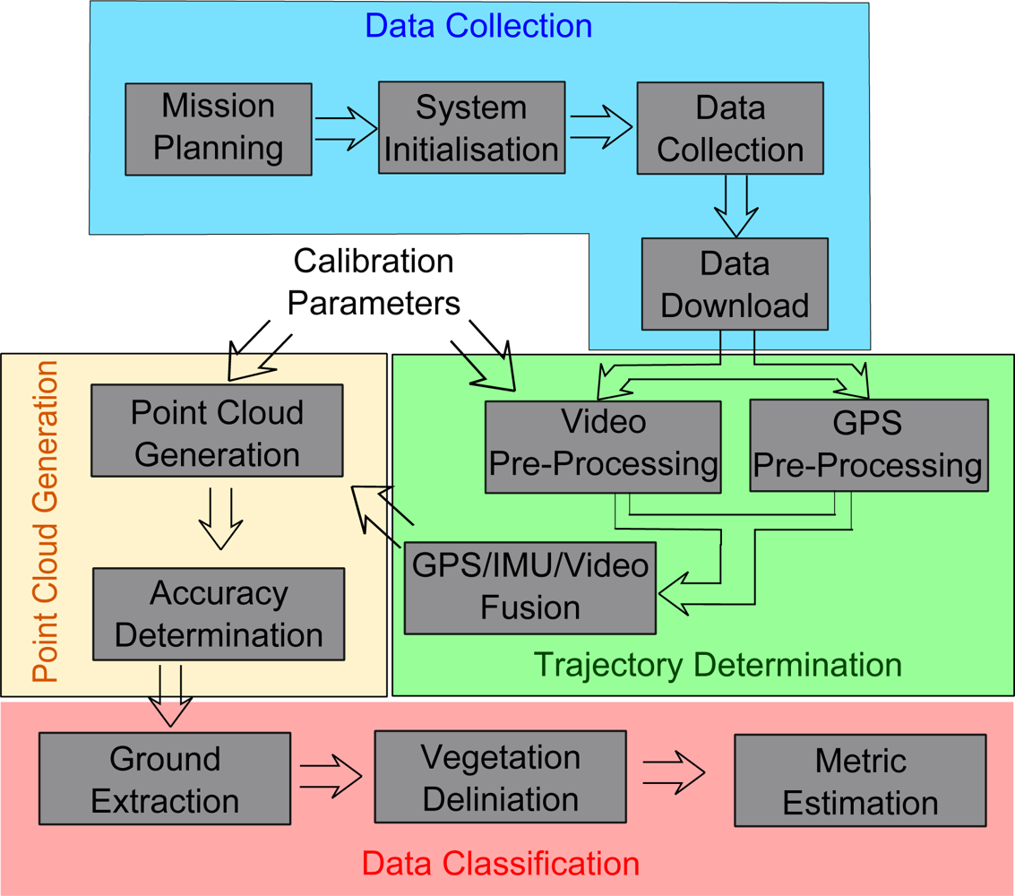
3.1. LiDAR Workflow
3.2. Trajectory Determination
3.2.1. Process Model
3.2.2. Observation Models
3.2.3. Sigma Point Kalman Smoother
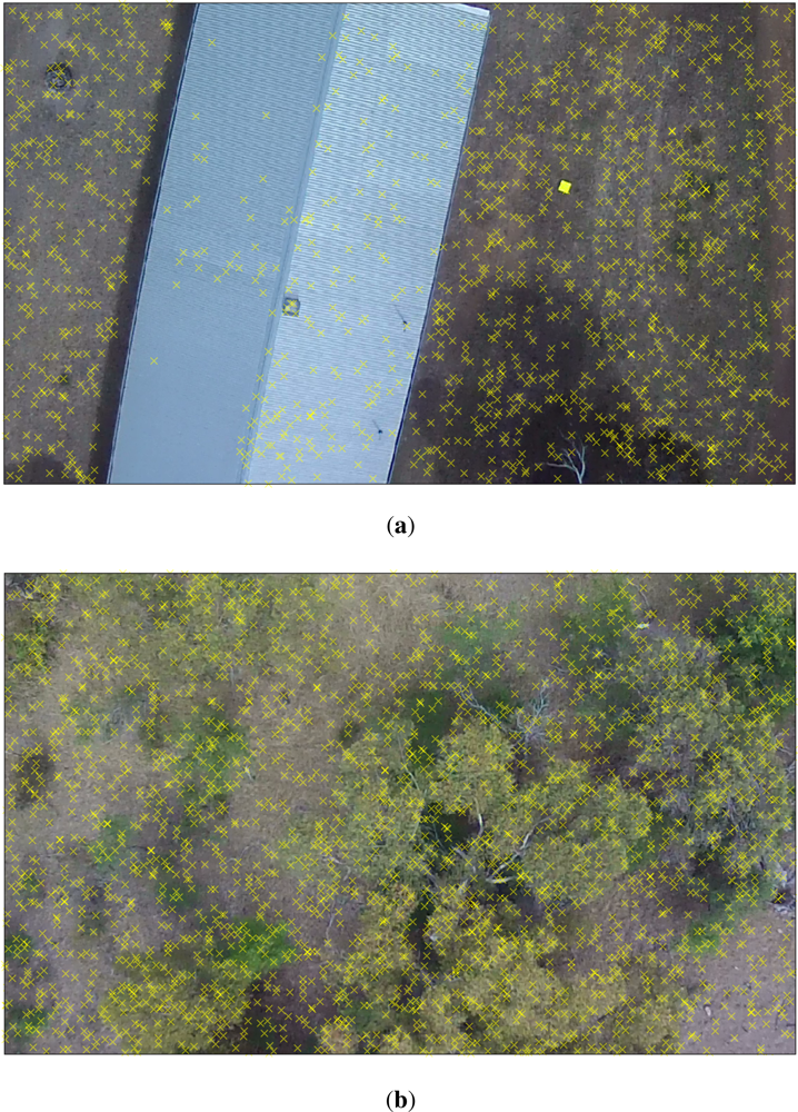
3.3. Calibration
3.4. Point Cloud generation and Accuracy Assessment
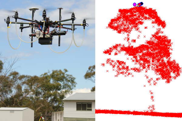
3.5. Individual Tree Metrics
4. Results and Discussion
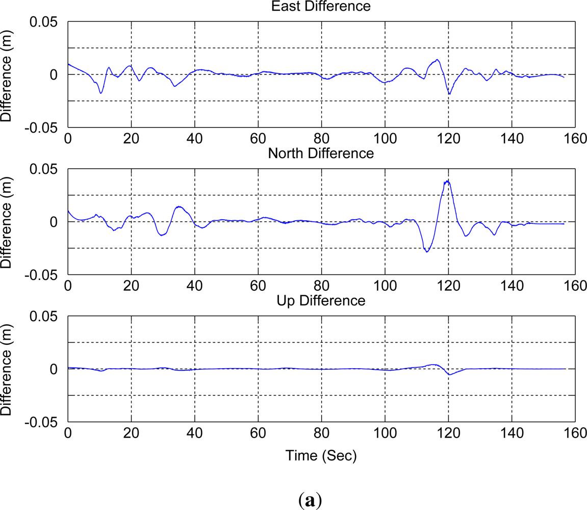
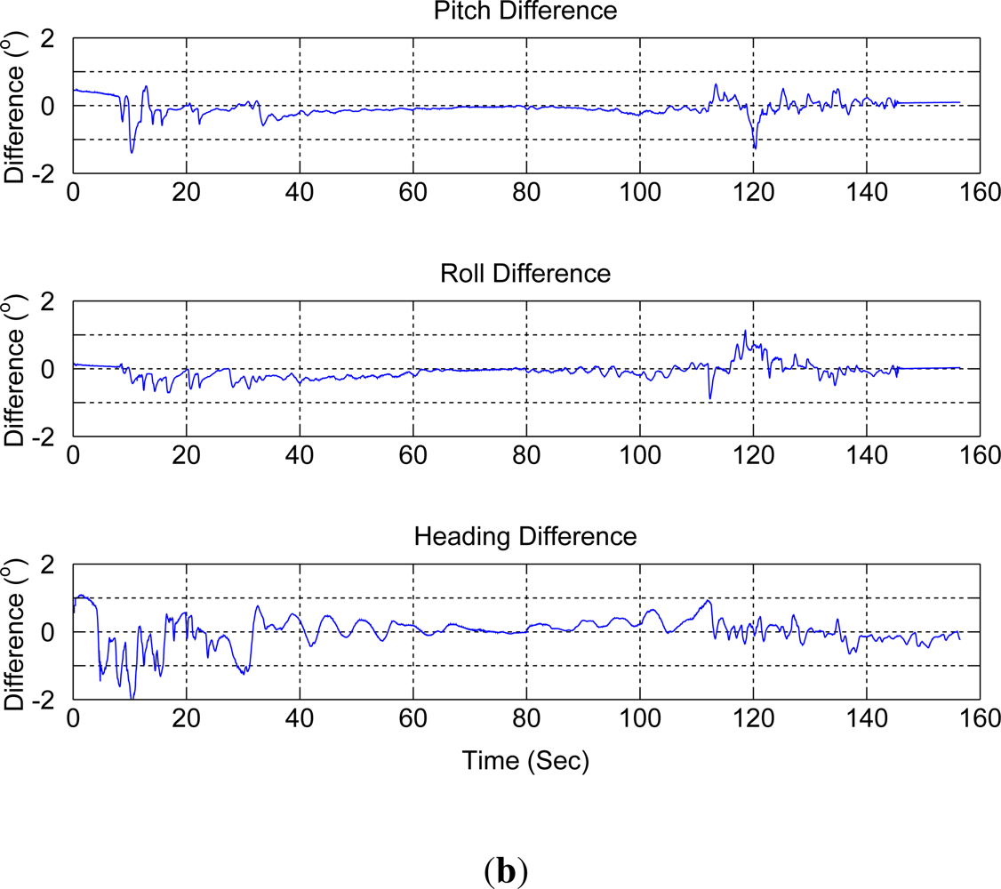
4.1. Trajectory Generation
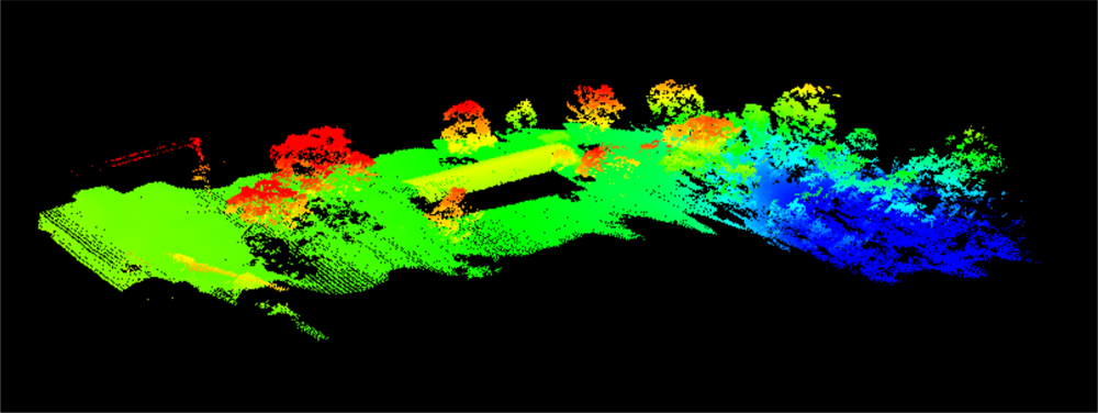
4.2. Point Cloud Properties
4.3. Point Cloud Accuracy
4.4. Individual Tree Metrics
5. Conclusions and Future Work
Acknowledgments
References
- Hyyppä, J.; Hyyppä, H.; Leckie, D.; Gougeon, F.; Yu, X.; Maltamo, M. Review of methods of small-footprint airborne laser scanning for extracting forest inventory data in boreal forests. Int J. Remote Sens 2008, 29, 1339–1366. [Google Scholar]
- Lefsky, M.; Cohen, W.; Parker, G.; Harding, D. Lidar remote sensing for ecosystem studies. Bioscience 2002, 52, 19–30. [Google Scholar]
- Akay, A.E.; Ouz, H.; Karas, I.R.; Aruga, K. Using LiDAR technology in forestry activities. Environ. Monit. Assess 2009, 151, 117–125. [Google Scholar]
- Erdody, T.L.; Moskal, L.M. Fusion of LiDAR and imagery for estimating forest canopy fuels. Remote Sens. Environ 2010, 114, 725–737. [Google Scholar]
- Morsdorf, F.; Nichol, C.; Malthus, T.; Woodhouse, I.H. Assessing forest structural and physiological information content of multi-spectral LiDAR waveforms by radiative transfer modelling. Remote Sens. Environ 2009, 113, 2152–2163. [Google Scholar]
- Lim, K.; Treitz, P.; Wulder, M.; St-Onge, B.; Flood, M. LiDAR remote sensing of forest structure. Prog. Phys. Geog 2003, 27, 88–106. [Google Scholar]
- Barazzetti, L.; Remondino, F.; Scaioni, M. Automation in 3D reconstruction: Results on different kinds of close-range blocks. Int. Arch. Photogramm., Remote Sens. Spat. Inf. Sci 2010, 38, 55–61. [Google Scholar]
- Chiabrando, F.; Nex, F.; Piatti, D.; Rinaudo, F. UAV and RPV systems for photogrammetric surveys in archaelogical areas: Two tests in the Piedmont region (Italy). J. Archaeol. Sci 2011, 38, 697–710. [Google Scholar]
- Sugiura, R.; Noguchi, N.; Ishii, K. Remote-sensing technology for vegetation monitoring using an unmanned helicopter. Biosyst. Eng 2005, 90, 369–379. [Google Scholar]
- Laliberte, A.S.; Goforth, M.A.; Steele, C.M.; Rango, A. Multispectral remote sensing from unmanned aircraft: Image processing workflows and applications for rangeland environments. Remote Sens 2011, 3, 2529–2551. [Google Scholar]
- Hunt, E., Jr; Hively, W.; Fujikawa, S.; Linden, D.; Daughtry, C.; McCarty, G. Acquisition of NIR-Green-Blue digital photographs from unmanned aircraft for crop monitoring. Remote Sens 2010, 2, 290–305. [Google Scholar]
- Tao, W.; Lei, Y.; Mooney, P. Dense Point Cloud Extraction from UAV Captured Images in Forest Area. Proceedings of the 2011 IEEE International Conference on Spatial Data Mining and Geographical Knowledge Services, Fuzhou, China, 29 June–1 July 2011; pp. 389–392.
- Dandois, J.P.; Ellis, E.C. Remote sensing of vegetation structure using computer vision. Remote Sens 2010, 2, 1157–1176. [Google Scholar]
- Jaakkola, A.; Hyyppä, J.; Kukko, A.; Yu, X.; Kaartinen, H.; Lehtomäki, M.; Lin, Y. A low-costmulti-sensoral mobile mapping system and its feasibility for tree measurements. ISPRS J. Photogramm 2010, 65, 514–522. [Google Scholar]
- Lin, Y.; Hyyppä, J.; Jaakkola, A. Mini-UAV-borne LIDAR for fine-scale mapping. IEEE Geosci. Remote S 2011, 8, 426–430. [Google Scholar]
- Choi, K.; Lee, I.; Hong, J.; Oh, T.; Shin, S. Developing a UAV-based rapid mapping system for emergency response. Proc. SPIE 2009, 7332, 733209–733209-12. [Google Scholar]
- Nagai, M.; Shibasaki, R.; Kumagai, H.; Ahmed, A. UAV-borne 3-D mapping system by multisensor integration. IEEE T. Geosci. Remote 2009, 47, 701–708. [Google Scholar]
- Miller, R.; Amidi, O. 3-D Site Mapping with the CMU Autonomous Helicopter 3-D Site Mapping with the CMU Autonomous Helicopter. Proceedings of the 5th International Conference on Intelligent Autonomous Systems, Sapparo, Japan, June 1998.
- Glennie, C. Rigorous 3D error analysis of kinematic scanning LIDAR systems. J. Appl. Geodes 2007, 1, 147–157. [Google Scholar]
- Schwarz, K.; El-Sheimy, N. Mobile Mapping Systems State of the art and future trends. Int. Arch. Photogr. Remote Sens. Spat. Inf. Sci 2004, 35, 10. [Google Scholar]
- El-sheimy, N. Emerging MEMS IMU and Its Impact on Mapping Applications; Photogrammetric Week: Stuttgart, Germany, 7–11 September 2009; pp. 203–216. [Google Scholar]
- Wallace, L.; Lucieer, A.; Turner, D.; Watson, C. Error assessment and mitigation for hyper-temporal UAV-borne LiDAR surveys of forest inventory. Proceedings of Silvilaser 2011, Hobart, Australia, 16–20 October 2011.
- Shin, E. An Unscented Kalman Filter for In-Motion Alignment of Low-Cost IMUs. Proceedings of Position Location and Navigation Symposium, Huntsville, AL, USA, 26–29 April 2004; pp. 273–279.
- El-Sheimy, N.; Chiang, K.W.; Noureldin, A. The Utilization of Artificial Neural Networks for Multisensor System Integration in Navigation and Positioning Instruments. IEEE T. Instrum. Meas 2006, 55, 1606–1615. [Google Scholar]
- Chiang, K.W.; Chang, H.W.; Li, C.Y.; Huang, Y.W. An artificial neural network embedded position and orientation determination algorithm for low cost MEMS INS/GPS integrated sensors. Sensors 2009, 9, 2586–2610. [Google Scholar]
- Bryson, M.; Sukkarieh, S. A Comparison of Feature and Pose-Based Mapping Using Vision, Inertial and GPS on a UAV. Proceedings of the 2011 IEEE/RSJ International Conference on Intelligent Robots and Systems (IROS), San Francisco, CA, USA, 25–30 September 2011; pp. 4256–4262.
- Andersen, E.; Taylor, C. Improving MAV Pose Estimation Using Visual Information. Proceedings of the IEEE/RSJ International Conference on Intelligent Robots and Systems, San Diego, CA, USA, 29 October–2 November 2007; pp. 3745–3750.
- Gajdamowicz, K.; Öhman, D.; Horemuz, M. Mapping and 3D Modelling of Urban Environment Based on Lidar, Gps/Imu and Image Data. Proceeding of 5th International Symposium on Mobile Mapping Technology, Padova, Italy, 28–31 May 2007.
- Snavely, N.; Seitz, S.M.; Szeliski, R. Photo tourism: exploring photo collections in 3D. ACM Trans. Graph 2006, 25, 835–846. [Google Scholar]
- Morsdorf, F.; Kötz, B.; Meier, E.; Itten, K.; Allgöwer, B. Estimation of LAI and fractional cover from small footprint airborne laser scanning data based on gap fraction. Remote Sens. Environ 2006, 104, 50–61. [Google Scholar]
- Zhang, H.; Wu, Y.; Wu, W.; Wu, M.; Hu, X. Improved multi-position calibration for inertial measurement units. Meas. Sci. Technol 2010, 21, 15107–15117. [Google Scholar]
- Bouget, J.Y. Camera Calibration Toolbox for Matlab. 2010. Available online: http://www.vision.caltech.edu/bouguetj/calib_doc/ (accessed on 12 January 2012).
- Van Der Merwe, R.; Wan, E. Sigma-Point Kalman Filters for Integrated Navigation. In Proceedings of the 60th Annual Meeting of the Institute of Navigation (ION), Dayton, OH, USA, 7–9 June 2004; pp. 641–654.
- Wan, E.; van der Merwe, R. The Unscented Kalman Filter for Nonlinear Estimation. In Proceedings of the IEEE 2000 Adaptive Systems for Signal Processing, Communications, and Control Symposium, Lake Louise, AB, Canada, 1–4 October 2000; pp. 153–158.
- Crassidis, J. Sigma-point Kalman filtering for integrated GPS and inertial navigation. IEEE T. Aero. Elec. Sys 2006, 42, 750–756. [Google Scholar]
- Gavrilets, V. Autonomous Aerobatic Maneuvering of Miniature Helicopters, 2003.
- Van Der Merwe, R. Sigma-Point Kalman Filters for Probabilistic Inference in Dynamic State-Space Models; PhD Thesis, Oregon Health and Science University, Portland, OR, USA; 2004. [Google Scholar]
- Dellaert, F.; Seitz, S.M.; Thorpe, C.E.; Thrun, S. Structure from Motion without Correspondence. Proceedings of the IEEE International Conference on Computer Vision and Pattern Recognition (CVPR), Hilton Head, SC, USA, 13–15 June 2000; pp. 2557–2564.
- Lowe, D. Distinctive image features from scale-invariant keypoints. Int. J. Comput. Vis 2004, 60, 91–110. [Google Scholar]
- Nistér, D. An efficient solution to the five-point relative pose problem. IEEE T. Pattern. Anal 2004, 26, 756–770. [Google Scholar]
- Hol, J.D.; Schon, T.B.; Gustafsson, F. Modeling and calibration of inertial and vision sensors. Int. J. Rob. Res 2010, 29, 231–244. [Google Scholar]
- Isenberg, M. LAStools—Efficient Tools for LiDAR Processing. 2011. Available online: http://www.cs.unc.edu/~isenburg/lastools/ (accessed on 15 December 2011).
- Shrestha, R.; Wynne, R.H. Estimating biophysical parameters of individual trees in an urban environment using small footprint discrete-return imaging lidar. Remote Sens 2012, 4, 484–508. [Google Scholar]
- Blanchard, S.D.; Jakubowski, M.K.; Kelly, M. Object-based image analysis of downed logs in disturbed forested landscapes using lidar. Remote Sens 2011, 3, 2420–2439. [Google Scholar]
- Adams, T. Remotely Sensed Crown Structure as an Indicator of Wood Quality. A Comparison of Metrics from Aerial and Terrestrial Laser Scanning. Proceedings of Silvilaser 2011, Hobart, Australia, 16–20 October 2011.
- Raber, G.; Jensen, J.; Hodgson, M.; Tullis, J.; Davis, B.; Berglund, J. Impact of lidar nominal post-spacing on DEM accuracy and flood zone delineation. Photogramm. Eng. Remote Sensing 2007, 7, 793–804. [Google Scholar]
- Goulden, T.; Hopkinson, C. The forward propagation of integrated system component errors within airborne lidar data. Photogramm. Eng. Remote Sensing 2010, 5, 589–601. [Google Scholar]
- Yu, X.; Hyyppä, J.; Holopainen, M.; Vastaranta, M. Comparison of area-based and individual tree-based methods for predicting plot-level forest attributes. Remote Sens 2010, 2, 1481–1495. [Google Scholar]


| Gyroscopes | Accelerometers | |
|---|---|---|
| Range | 50°/s | 1.7g |
| Non-linearity | 0.2% | 0.2% |
| Bias Stability | 0.2°/s | 0.003g |
| Flight | Flight Time (s) | Mean Height (m) | Mean Horizontal Velocity (m/s) | Primary Heading (deg) | Key Frames/s |
|---|---|---|---|---|---|
| 1 | 161 | 48 | 3.77 | 180 | 2.3 |
| 2 | 137 | 54 | 3.27 | 90 | 1.8 |
| 3 | 130 | 46 | 3.16 | 135 | 1.9 |
| 4 | 195 | 44 | 3.33 | 225 | 1.8 |
| Transect | Area (m2) | Point Density (ppm2) | % 2nd Returns | % 3rd Returns |
|---|---|---|---|---|
| 1a | 5, 931 | 38.7 | 4.09 | 0.35 |
| 1b | 6, 288 | 37.2 | 5.88 | 0.53 |
| 2a | 5, 586 | 62.6 | 3.46 | 0.54 |
| 2b | 4, 922 | 42.2 | 13.90 | 2.05 |
| 3a | 5, 459 | 35.9 | 15.01 | 2.02 |
| 3b | 4, 986 | 36.5 | 15.41 | 2.37 |
| 4a | 6, 176 | 40.6 | 2.92 | 0.25 |
| 4b | 5, 811 | 52.0 | 2.63 | 0.17 |
| (a) | |||||||||
|---|---|---|---|---|---|---|---|---|---|
| Flight | No. Targets | East (m) | North (m) | Up (m) | RMSE (m) | ||||
| Mean (m) | σ (m) | Mean (m) | σ (m) | Mean (m) | σ (m) | Hor. (m) | Vert. (m) | ||
| 1a | 16 | −0.11 | 0.23 | 0.26 | 0.21 | 0.11 | 0.23 | 0.57 | 0.24 |
| 1b | 14 | 0.22 | 0.40 | −0.13 | 0.31 | −0.02 | 0.07 | 0.62 | 0.07 |
| 2a | 17 | 0.08 | 0.59 | −0.06 | 0.33 | 0.09 | 0.22 | 0.66 | 0.23 |
| 2b | 16 | −0.13 | 0.42 | −0.10 | 0.21 | 0.01 | 0.05 | 0.48 | 0.05 |
| 3a | 16 | −0.17 | 0.55 | 0.18 | 0.34 | 0.27 | 0.09 | 0.85 | 0.29 |
| 3b | 17 | −0.04 | 0.14 | 0.30 | 0.24 | 0.07 | 0.10 | 0.40 | 0.12 |
| 4a | 15 | −0.06 | 0.50 | −0.05 | 0.54 | 0.00 | 0.17 | 0.70 | 0.16 |
| 4b | 18 | −0.13 | 0.37 | 0.15 | 0.42 | −0.00 | 0.20 | 0.58 | 0.19 |
| all | 130 | −0.03 | 0.41 | 0.07 | 0.42 | 0.06 | 0.18 | 0.60 | 0.19 |
| Expected | 0.54 | 0.16 | |||||||
| (b) | |||||||||
|---|---|---|---|---|---|---|---|---|---|
| Flight | No. Targets | East (m) | North (m) | Up (m) | RMSE (m) | ||||
| Mean (m) | σ (m) | Mean (m) | σ (m) | Mean (m) | σ (m) | Hor. (m) | Vert. (m) | ||
| 1a | 17 | 0.02 | 0.11 | −0.12 | 0.27 | −0.02 | 0.14 | 0.38 | 0.15 |
| 1b | 14 | 0.13 | 0.15 | −0.05 | 0.24 | 0.09 | 0.08 | 0.41 | 0.12 |
| 2a | 17 | −0.03 | 0.25 | 0.03 | 0.06 | 0.04 | 0.14 | 0.35 | 0.17 |
| 2b | 16 | −0.04 | 0.12 | −0.06 | 0.07 | −0.00 | 0.03 | 0.21 | 0.03 |
| 3a | 16 | −0.19 | 0.32 | 0.08 | 0.08 | 0.05 | 0.13 | 0.34 | 0.16 |
| 3b | 17 | 0.09 | 0.12 | 0.17 | 0.22 | 0.11 | 0.14 | 0.31 | 0.17 |
| 4a | 15 | 0.02 | 0.30 | −0.17 | 0.24 | −0.04 | 0.09 | 0.41 | 0.10 |
| 4b | 18 | −0.03 | 0.22 | 0.02 | 0.26 | −0.06 | 0.15 | 0.33 | 0.16 |
| all | 130 | 0.01 | 0.17 | −0.01 | 0.21 | 0.03 | 0.12 | 0.32 | 0.14 |
| Expected | 0.26 | 0.15 | |||||||
| (a) | ||||||
|---|---|---|---|---|---|---|
| Tree | Measurement Count | Location | Height (m) | Width (m) | ||
| σ (m) | Mean (m) | σ (m) | Mean (m) | σ (m) | ||
| 1 | 6 | 0.44 | 10.94 | 0.05 | 8.26 | 0.25 |
| 2 | 4 | 0.59 | 11.49 | 0.13 | 11.53 | 0.35 |
| 3 | 3 | 0.55 | 12.71 | 0.11 | 12.93 | 1.02 |
| 4 | 5 | 0.56 | 14.65 | 0.25 | 14.39 | 0.54 |
| (b) | ||||||
|---|---|---|---|---|---|---|
| Tree | Measurement Count | Location | Height (m) | Width (m) | ||
| σ (m) | Mean (m) | σ (m) | Mean (m) | σ (m) | ||
| 1 | 6 | 0.47 | 10.85 | 0.10 | 7.77 | 0.32 |
| 2 | 4 | 0.73 | 11.25 | 0.25 | 11.21 | 0.54 |
| 3 | 3 | 0.74 | 12.56 | 0.35 | 12.92 | 1.18 |
| 4 | 5 | 1.14 | 14.47 | 0.31 | 14.10 | 0.36 |
Share and Cite
Wallace, L.; Lucieer, A.; Watson, C.; Turner, D. Development of a UAV-LiDAR System with Application to Forest Inventory. Remote Sens. 2012, 4, 1519-1543. https://doi.org/10.3390/rs4061519
Wallace L, Lucieer A, Watson C, Turner D. Development of a UAV-LiDAR System with Application to Forest Inventory. Remote Sensing. 2012; 4(6):1519-1543. https://doi.org/10.3390/rs4061519
Chicago/Turabian StyleWallace, Luke, Arko Lucieer, Christopher Watson, and Darren Turner. 2012. "Development of a UAV-LiDAR System with Application to Forest Inventory" Remote Sensing 4, no. 6: 1519-1543. https://doi.org/10.3390/rs4061519
APA StyleWallace, L., Lucieer, A., Watson, C., & Turner, D. (2012). Development of a UAV-LiDAR System with Application to Forest Inventory. Remote Sensing, 4(6), 1519-1543. https://doi.org/10.3390/rs4061519