Article

Sensor Correction of a 6-Band Multispectral Imaging Sensor for UAV Remote Sensing

School of Geography and Environmental Studies, University of Tasmania, Private Bag 76, Hobart, TAS 7001, Australia
*
Author to whom correspondence should be addressed.
Remote Sens. 2012, 4(5), 1462-1493; https://doi.org/10.3390/rs4051462
Submission received: 28 March 2012 / Revised: 20 April 2012 / Accepted: 4 May 2012 / Published: 18 May 2012
(This article belongs to the Special Issue Unmanned Aerial Vehicles (UAVs) based Remote Sensing)

Abstract

:
Unmanned aerial vehicles (UAVs) represent a quickly evolving technology, broadening the availability of remote sensing tools to small-scale research groups across a variety of scientific fields. Development of UAV platforms requires broad technical skills covering platform development, data post-processing, and image analysis. UAV development is constrained by a need to balance technological accessibility, flexibility in application and quality in image data. In this study, the quality of UAV imagery acquired by a miniature 6-band multispectral imaging sensor was improved through the application of practical image-based sensor correction techniques. Three major components of sensor correction were focused upon: noise reduction, sensor-based modification of incoming radiance, and lens distortion. Sensor noise was reduced through the use of dark offset imagery. Sensor modifications through the effects of filter transmission rates, the relative monochromatic efficiency of the sensor and the effects of vignetting were removed through a combination of spatially/spectrally dependent correction factors. Lens distortion was reduced through the implementation of the Brown–Conrady model. Data post-processing serves dual roles in data quality improvement, and the identification of platform limitations and sensor idiosyncrasies. The proposed corrections improve the quality of the raw multispectral imagery, facilitating subsequent quantitative image analysis.

Graphical Abstract

1. Introduction

Unmanned aerial vehicles (UAVs) are gaining attention from the scientific community as novel tools for remote sensing applications [1]. Compared with more traditional aircraft or satellite based platforms, the UAV fills a previously unoccupied niche due to the unique characteristics of data it is able to capture. Its low operating altitude allows for the generation of ultra-high spatial resolution data over relatively small spatial extents [2] (see Figure 1). Furthermore, the greatly reduced preparation time of UAVs relative to large scale platforms aids in the acquisition of multi-temporal datasets or in exploiting limited windows of opportunity [3]. UAVs may serve to bridge the scale gap between satellite imagery, full-scale aerial photography, and field samples.
The UAV offers an unprecedented level of accessibility to and control over a remote sensing platform. Progress within the fields of digital sensors, navigational equipment, and small-scale aircraft have all reduced the cost of the fundamental components of UAVs [4]. With the growing availability of relatively low-cost commercial components, small-scale research groups are now presented with the alternative of developing their own UAV-based projects. A wide selection of digital sensors allows researchers to cater systems for their own specific research requirements. This flexibility is being demonstrated in a growing number of remote sensing UAV studies. Berni et al. [5], Lelong [6], Dunford et al. [2], Hunt et al. [7], Laliberte et al. [8], and Xiang and Tian [9] looked at multispectral UAV imagery for both agricultural monitoring and natural vegetation classification. Zhao et al. [10] and Lin et al. [11] used UAV-based LiDAR for topographic modelling and feature identification. UAVs were used for stereo-image 3D landscape modelling by Stefanik et al. [12]. Thermal UAV applications for emergency services including bushfires and search and rescue were presented by Rudol and Doherty [13], Hinkley and Zajkowski [14] and Pastor et al. [15]. Temporal mapping of landscape dynamics was reviewed by Walter et al. [16].
The increase in accessibility of UAV platforms requires an increase in skillsets for research groups. Technical skills are required that cover all aspects of platform development, data post-processing, and image analysis. In response to this requirement, workflow methodologies for approaching developmental aspects of UAV construction are being formulated. For example, in this special issue Laliberte et al. [17] demonstrates a UAV workflow for rangeland UAV monitoring.
The objective of this study is to provide a primarily image-based, linear workflow of the sensor correction of a low-cost consumer grade multispectral sensor. In addition to providing a practical context for the theoretical background of sensor correction, our study will highlight the advantages, limitations, and pitfalls associated with UAV-based multispectral remote sensing through:
  • identification, assessment and quantification of the components of data modification within a consumer level multispectral sensor;
  • implementation of image-based radiometric correction techniques; and
  • assessment of post-radiometric correction data quality issues.

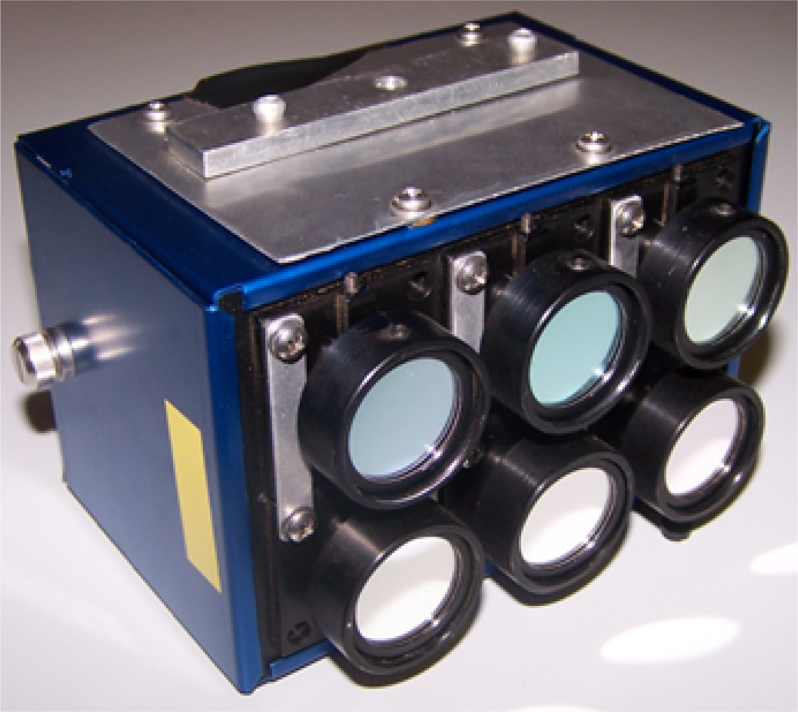
1.1. UAV Multispectral Sensors

Despite the opportunities provided by UAVs, both hardware and software limitations result in some compromises. As a remote sensing platform, the UAV is relatively limited in both its payload capacity and flight duration [4]. It is necessary to balance platform accessibility with the technological limitations inherent of small-scale platforms and the data quality of low-cost sensors. Such cost and weight limitations necessitate a reduction in manufacturing quality of the sensor. Reductions are readily achieved through the use of cheaper construction materials and methods, limited data storage capacity, or the absence of on-board processing features.
Multispectral sensors offer powerful opportunities for environmental remote sensing with UAV platforms. A multispectral sensor collects spectral data from multiple discrete bands of the electromagnetic spectrum. The flexibility of multispectral sensors arises from the user’s ability to preselect and/or interchange the spectral filter elements within individual channels, thereby allowing for the strategic targeting of specific bands of the spectrum [18]. A wealth of literature has established the value of spectral indices derived from multispectral data for the extraction of physical or biophysical information from spectral data. Glenn et al. [19] demonstrates the use of vegetation indices as proxies for other vegetative biophysical information. A comparative study by Lacava et al. [20] between field measurements and remotely sensed data revealed the value of spectrally derived wetness indices for estimating soil moisture.
The miniature camera array (mini-MCA) is a relatively low-cost consumer level six-band multispectral sensor available from Tetracam inc. ( http://www.tetracam.com/). The mini-MCA consists of an array of six individual channels, each consisting of a CMOS sensor with a progressive shutter, an objective lens, and mountings for interchangeable band-pass filters. The mini-MCA Channels are labeled from “1” to “5”, while the sixth “master” channel is used to define the global settings used by all channels (e.g., integration time). Image data is collected at a user-definable dynamic range of either 8 or 10 bits. Provided factory standards detail the relative monochromatic response of the CMOS across the visible and NIR wavelengths. In-house modifications made to the mini-MCA include UAV mountings and alterations to the bandpass filter holders to allow for easier interchange of the filters (see Figure 2).
Each of the mini-MCA channels is equipped with mountings for the fitting of interchangeable 1″ band-pass filters. The mini-MCA is purchased with six filters preselected by the user. An additional six band-pass filters were obtained from Andover corporation ( http://www.andovercorp.com/). These twelve 10 nm bandwidth filters were selected from across the visible and NIR wavelengths with close regard to known biophysical indices developed for environmental monitoring purposes [21].
Raw at-sensor data has been modified by a combination of effects that include surface conditions, atmospheric effects, topographic effects and sensor characteristics [22,23]. These effects obscure the true surface reflectance properties and diminish the capacity to extract accurate quantitative information from remotely sensed imagery. Radiometric post-processing encompasses the suite of techniques to extract spatially consistent surface reflectance values from the raw data and is conducted across two main phases: sensor correction and radiometric calibration.
Sensor corrections and radiometric calibration are sequential steps in the task to extract high quality reflectance data (see Figure 3). Sensor correction encompasses the methods used to extract geometrically consistent at-sensor measurements from the raw data. The focus of this initial phase is therefore upon reducing sensor-based data modifications. Radiometric calibration further builds upon the correction results by deriving at-surface reflectance from these at-sensor measurements. This is achieved through the calibration of data with regard to the environmental conditions present during data collection [24]. The primary focus of this study is on the preliminary corrections for sensor correction. A single multispectral image provides a case study to illustrate the effects of sensor corrections.

2. Methods

Raw at-sensor data values represent arbitrary units of highly modified at-sensor measurements [22]. These modifications may occur during the collection, processing, and transmission of data by the sensor system [25], and include processes that either introduce unwanted additional measurements or directly alter the strength or spatial properties of the incoming radiance [22,26]. Sensor correction encompasses the suite of techniques for correcting these sensor based processes, allowing the extraction of arbitrary digital numbers (DN). Raw data conversion, processing and sensor correction application were conducted using IDL script within the ENVI software package ( http://www.ittvis.com/). Raw mini-MCA data was converted into individual 10 bit image bands.

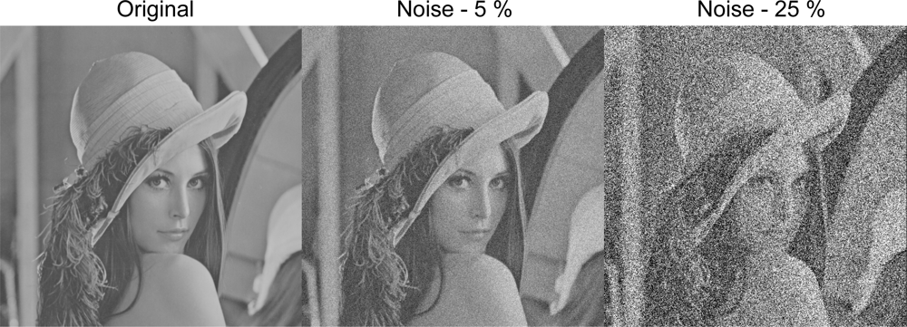
2.1. Noise Correction

Small, low-cost sensors are prone to the effects of noise. Noise collectively refers to erroneous sensor measurements generated independently to collected radiance, therefore representing an additive source of error to the data [25]. Noise is characterised into two broad components: systematic and random. Systematic noise represents a source of bias consistent in both its value and spatial properties. Conversely, random noise refers to the introduction of non-correlated, non-reproducible noise that varies randomly over time [26]. Noise reduction techniques include image-based approaches [26] and signal processing techniques that are used to isolate high frequency non-correlated data components [25,27].
The value of each pixel within the raw data represents the sum of a radiance component and a noise component (Equation (1)). The larger the proportion of noise within the image data, the more obscured the true radiance component becomes (see Figure 4). The separation of this radiance component requires some form of quantification of the contribution of the noise components to the raw data.
D N raw = D N rad + D N n
Noise itself is broadly comprised of random and systematic components. Random noise refers to non-correlated, non-reproducible noise that varies randomly [26]. The uncertainty of the exact contribution of this random noise component limits noise removal techniques. Given its temporally random properties, the exact contribution of the random component to the value of a pixel at any given moment is unknown and cannot be accurately separated from the radiance component (Equation (2)). Noise correction techniques are therefore forced to focus upon reductive techniques rather than outright removal. Knowledge of the per-pixel noise distribution characteristics are key for approximating the contribution of random noise.
D N raw = D N rad + ( D N sn + D N rn )

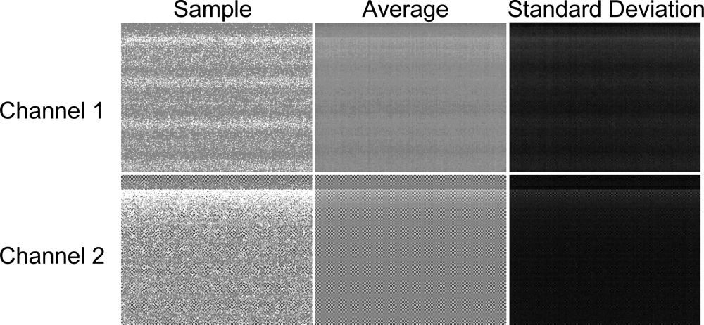
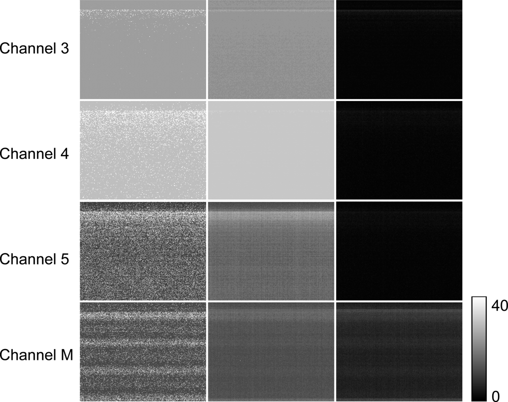
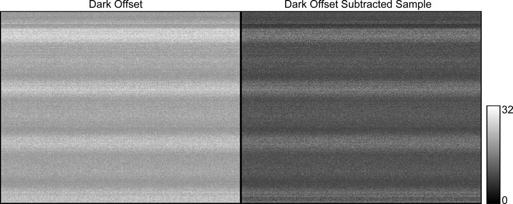
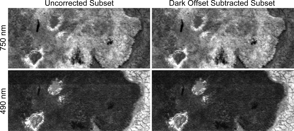
2.1.1. Dark Offset Subtraction

Characterisation of the noise component exploits its independent origin from the radiance component. Through the physical isolation of the sensor from incoming radiance, the radiance component can be globally reduced to zero. Dark offset imagery is raw image data generated such that it contains only the noise component [26,28]. Each dark offset image represents a single sample of the per-pixel noise within the sensor. Through repetition, a sensor-specific database of dark offset imagery can be constructed and characteristics of the per-pixel distribution of noise extracted. Dark offset subtraction is the subtraction of the per-pixel mean value of these noise distributions from image data. The standard deviation of the distribution provides a new measure of noise that, on average, will remain following dark offset subtraction. However, this standard deviation as a measure of noise may represent either an additive or subtractive offset to a pixels true value.

2.1.2. Dark Offset Image Generation Methodology

Dark offset imagery was generated for the mini-MCA within a dark room. To ensure radiance was excluded from the mini-MCA, it was first covered with a protective cloth before envelopment with a tightly fitting Gore-Tex hood. This setup was found to be both practical and capable of blocking incoming radiance across the relevant visible and NIR wavelengths.
Dark offset sample images were generated for each of the six mini-MCA channels at multiple exposure levels ranging from 1,000 μs to 20,000 μs (at 1,000 μs increments). For each 1,000 μs exposure step, 125 dark offset sample images were generated for each of the six channels. The per-pixel average and standard deviations were calculated for each combination of sensor and exposure and stored as separate images.

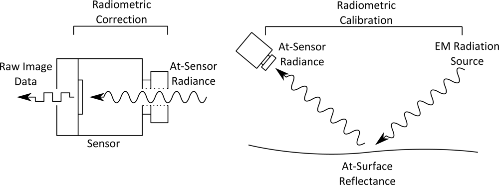
2.2. Radiance Strength Modification

Modifications to radiance strength within a sensor exhibit either a spectral or spatial dependency. Spectrally dependent processes include both filter transmittance and the monochromatic response of the sensor. Conversely, vignetting is a spatially dependent reduction of illumination strength dependent upon the angle of incoming radiance.

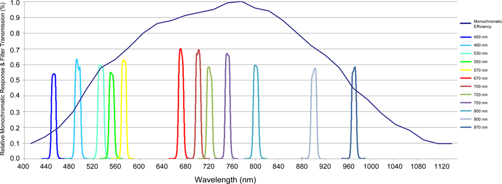
2.2.1. Monochromatic Response

Sensors exhibit additional non-uniformity to spectral response due to the effects of quantum efficiency. Sensors are dependent upon the photoelectric effect to generate charges from which to construct image data. Not every photon, however, generates a charge. Quantum efficiency defines the proportion of incoming photons capable of liberating electrons through the photoelectric effect [28]. The quantum efficiency of sensors varies both between materials and across wavelengths, therefore altering the amount of incoming radiance required to generate a proportionate charge between differing bandpass filters. Factory standards of the relative monochromatic response of the mini-MCA effectively describe the quantum efficiency across the visible and NIR spectrum (450 nm to 1,100 nm) (see Figure 5).

2.2.2. Filter Transmittance

The mini-MCA provides multispectral functionality through mountings for spectral bandpass filters. These filters, however, neither exhibit 100 % transmittance across their functional wavelength nor define discrete limits of equal spectral sensitivity. Instead, they exhibit variation in both spectral sensitivity over their defined bandwidth and transmission level between filters at different wavelengths. Factory standards for the acquired 12 bandpass filters express the transmission rate of each individual filter, exhibiting a range of signal transmission rates as high as 70 % for the 670 nm filter to as low as 55 % for the 450 nm filter (see Figure 5).
The combined effect of filter transmission rate and monochromatic efficiency results in a wavelength dependent global reduction in radiance strength (Equation (3)). This has effects both within and between bands in the mini-MCA. Reducing the radiance component increases the overall contribution of noise in the raw data. As such, filter selection strongly influences the signal-to-noise ratio (SNR) within the final data. Inter-band relationships are degraded through the wavelength dependent reductions in radiance, generating disproportionate relationships between bands of high/low radiance modification.
D N raw = D N rad * F T λ * M E λ + ( D N sn + D N rn )
Little can be done to address the disproportionate noise. The correct future application of radiometric calibration techniques will compensate for disproportionate inter-band relationships. Studies that lack a suitable radiometric calibration approach, and are therefore limited to analysing either DN or at-sensor radiance measurements, require the separate calculation and application of gains in order to restore the at-sensor radiance measurements. Given that the two processes are both global reductions in radiance strength dependent on wavelength, the simplest approach is the calculation of a single correction value. This value is specific to both filter and sensor and is derived from multiplicative effects of both transmission and efficiency rates. Each image band is then globally multiplied by the corresponding correction factor.

2.3. Wavelength Dependent Correction Factor Methodology

Wavelength dependent correction factors were calculated from a combination of filter transmission and monochromatic efficiency. For simplicity, the detector was assumed to exhibit a linear response to radiance. The combined reduction in transmission rate was calculated over a 10 nm bandwidth from the factory standard values provided by Andover. An estimation of the relative monochromatic response was estimated from the information provided by TetraCam (see Table 1).

2.3.1. Flat Field Correction Factors

Vignetting is defined as a spatially dependent light intensity falloff that results in a progressive radial reduction in radiance strength towards the periphery of an image [2931]. The primary source of vignetting arises from differences in irradiance across the image plane due to the geometry of the sensor optics. Widening angles increase the occlusion of light, leading to a radial shadowing effect as illumination is reduced (see Figure 6). For a thorough review of the additional sources that contribute to the vignetting effect see Goldman [29].
The two broad methods to vignetting correction involve either modelling the optical pathway or image-based techniques. Methods based upon modelling the optical pathway use characteristics of the sensor to derive a model to describe vignetting falloff. This model can then be applied to imagery to compensate for illumination reduction due to the effects of vignetting.
Image-based approaches to vignetting correction typically rely upon the generation of a per-pixel correction factor look-up-table (LUT). Relative to optical modelling approaches, image based LUTs are arguably both simpler to calculate and more accurate [32]. LUTs require no knowledge of the optical pathway and represent the cumulative effects, including radial asymmetry, that contribute to the vignetting effect. Their overall development and application is, however, more time consuming, as any alteration to the vignetting pattern requires the generation of a new LUT.
Correction factor LUTs are generated from a uniform, spectrally homogeneous, Lambertian surface known as a flat field. Within the generated flat field imagery, deviation away from the expected uniform surface is attributed to the radial falloff effect of vignetting. A quantitative assessment of the per-pixel illumination falloff within the flat field image may be calculated and corresponding correction factor imagery generated. Correction factor images are calculated on the assumption that the brightest pixel within the image represents the true radiance measurement free from the effects of vignetting. A multiplicative correction factor is then calculated for each pixel, based on its difference with this true radiance measurement (Equation (4)) [32].
V LUT ( i , j ) = V FF ( i , j ) V FF max
A single flat field LUT corrects only for the vignetting characteristics present when the image was generated (Equation (5)). The quality of vignetting correction is degraded should variations in vignetting origin or rate of illumination falloff occur. Therefore the flat field LUT approach requires the identification of sources that generate variation within the vignetting effect. Although the aperture and focal lengths are known modifiers, both factors are fixed within the mini-MCA. Potential sources of vignetting variation include subtle variation between channels, exposure length and filters. The effect of individual channels were investigated by generating LUTs for each channel under equal conditions (i.e., filterless, equal exposure length). The effects of exposure length were investigated by generating LUTs from a single filterless channel across a range of exposure lengths. Finally, the effect of filters were investigated through a comparative investigation of filter and filterless LUTs upon a single channel.
D N raw = D N rad * F T λ * M E λ * V LUT ( i , j ) + ( D N sn + D N rn )

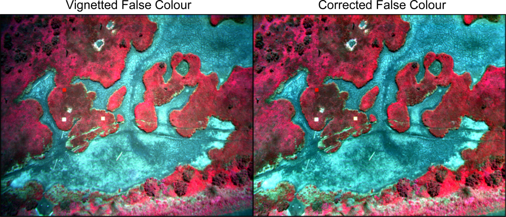
2.3.2. Vignetting Correction Methodology

A white artists canvas was selected to serve as the flat field surface due to its clear white homogeneous near-Lambertian surface. Flat field images were generated within a dark room with the white canvas evenly illuminated. In order to maximise the noise reduction potential of the dark offset subtraction process, each final flat field image was generated from the average of 125 flat field sample images. This process averages the random noise component within the data, thereby improving the correspondence of noise levels between the flat field image and the dark offset imagery. Correction factor images (i.e., LUTs) were then calculated from the noise-reduced average flat field image.

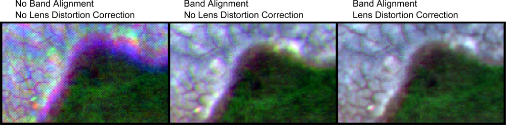
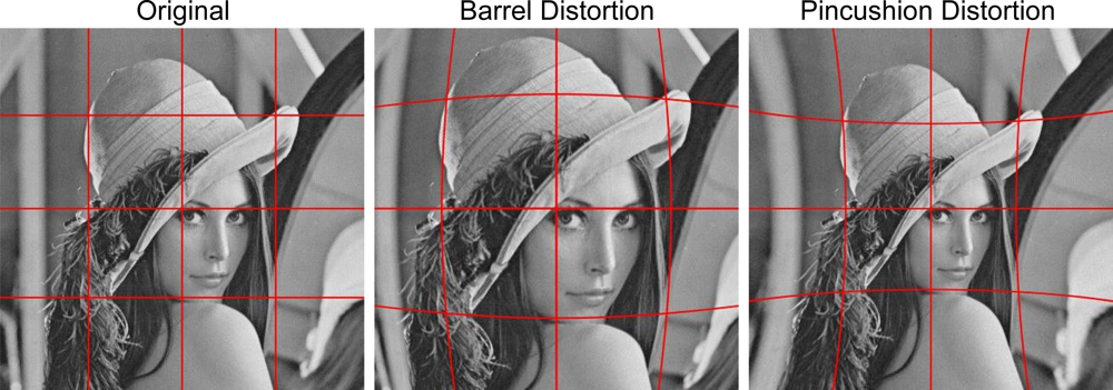
2.4. Lens Distortion

Lens distortion is mainly generated through a combination of differences in magnification level across a lens surface and misalignment between lens and the detector plane. These two factors result in a radially dependent geometric shift in a measurement position [3335]. Lens distortion is commonly represented by two components: radial distortion and tangential distortion [33]. Radial distortion represents the curving effect generated by subtle radial shift in magnification towards the centre of the lens, manifesting as a radial shift in value position (see Figure 7). Negative displacement radially shifts points towards the origin point of lens distortion, resulting in pincushion distortion effect. Conversely positive displacement shifts points away from the lens distortion origin, resulting in a barrel distortion effect [36,37]. Tangential distortion arises from the non-alignment of the lens with the CMOS resulting in a planar shift in the perspective of an image [33].

2.4.1. Brown–Conrady Model

A commonly adopted model for lens distortion is the Brown–Conrady distortion model [35,38,39]. The Brown–Conrady model is capable of calculating both the radial and tangential components of lens distortion. The model utilises an even-order polynomial model to calculate the radial displacement of a given image point. It is commonly recommended this polynomial is limited to the first two terms of radial distortion as higher order terms are insignificant in most cases.
The Brown–Conrady model requires prior calculation of radial and tangential distortion coefficients. An accessible approach for the calculation of the coefficients is the utilisation of a planar calibration grid of known geometric properties. Multiple images are generated of the calibration grid from different orientations. An iterative process then estimates both the intrinsic and extrinsic camera parameters based upon point correspondence between the known geometric properties of the scene and the distorted points within the image.

2.4.2. Lens Distortion Correction Methodology

Agisoft Lens is a freely available software package that utilises planar grids to calculate the Brown–Conrady coefficients. The calibration grid was displayed upon a 24″ flat panel LCD screen. Imagery of the calibration grid was captured by a filter-free mini-MCA at multiple angles. For each angle, multiple images were collected and averaged in order to maximise noise reduction. Filter-free vignetting correction factors were applied to the corresponding channel. Agisoft Lens was then used to calculate the lens distortion coefficients for each channel based upon the Brown–Conrady model.

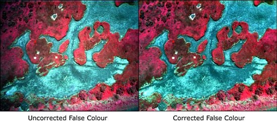
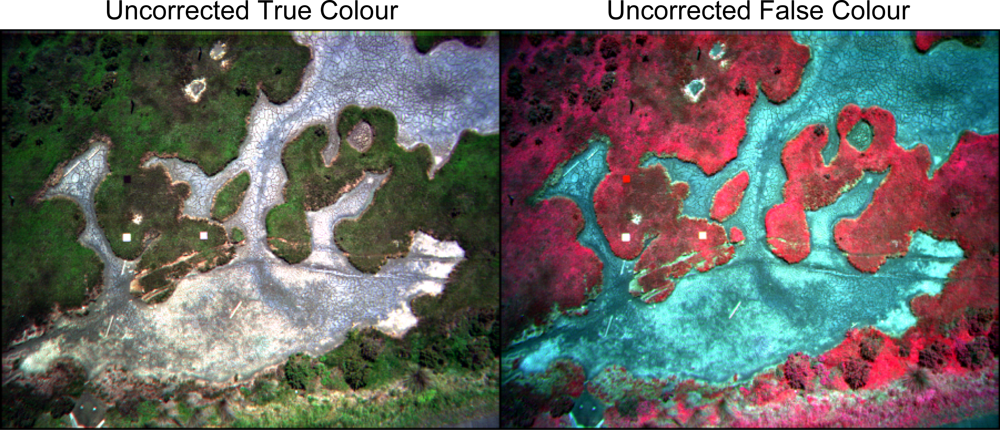
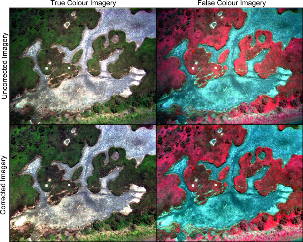
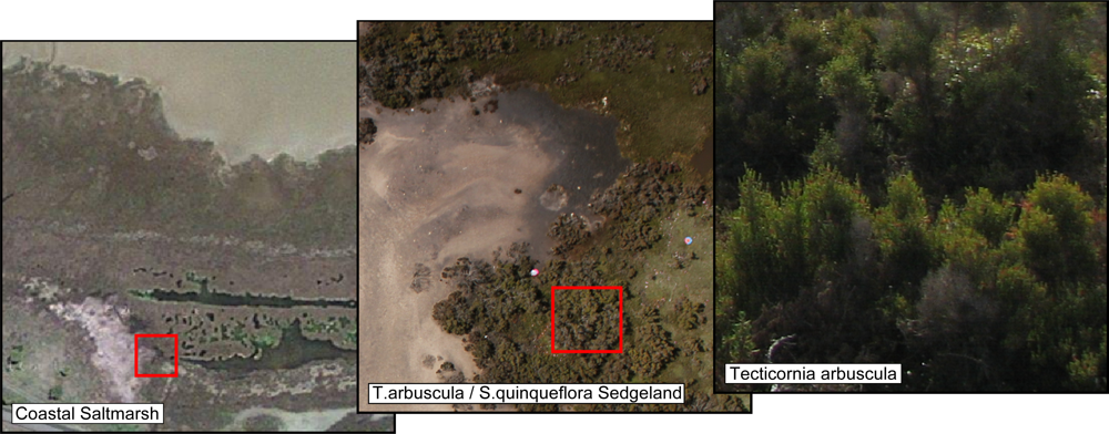
2.5. Salt Marsh Case Study

Salt marsh is predominately a coastal vegetation type characterised by herbaceous or low woody plants [40] that exhibit a tolerance towards water logging and/or saline conditions [41]. Salt marshes establish in regions where gentle topographic gradients that exist between the land and sea undergo periodic seawater inundation [42]. Plant communities within salt marshes often exhibit marked zonation in their distribution. It has been hypothesised that this is due to factors of drainage and salinity, and that increasing gradients of salt and water logging result in the successive elimination of species based upon tolerance [41]. The limited vertical stratification and relative topographic flatness of salt marsh communities represents an ideal, simplified environment within which to conduct preliminary UAV studies.
UAV imagery of salt marsh communities was acquired from the foreshore of Ralphs Bay, Australia. Six band multispectral data was captured using the mini-MCA mounted upon an Oktocopter UAV frame (see Table 2). Six bandpass filters were selected: 490, 530, 570, 670, 700 and 750 nm. A single multispectral image was selected to serve as a worked example of sensor corrections. The remaining imagery was reserved for a future UAV salt marsh study.

3. Results

3.1. Dark Offset Subtraction

Dark offset samples were generated for each channel of the mini-MCA. A preliminary visual assessment illustrates the similarities and differences in noise value, variation, and structure between the channels (see Figure 8). Three prominent manifestations of noise are exhibited: global checkered pattern, horizontal band noise, and strong periodic noise within channels 1 and M.

3.1.1. Global Checkered Pattern

Examination of the average per-pixel noise value and standard deviation reveals a bimodal distribution across the dark offset imagery (see Figure 9). A close visual inspection of the imagery reveals an alternating per pixel bias in the structure of the noise. This bimodal distribution is most strongly evident within channel 2, while the overlapping distributions of channel 1 only become clear within an examination of the differing standard deviations. Imagery was divided into two separate images based upon alternating pixels, with histograms of each of the alternating pixel states illustrating a clear separation of the bimodal distribution into two distinct distributions (see Figure 10).
The dual states within the channels raises two considerations with regard to noise: the potential for noise reduction of individual states and the introduction of psuedo-texture. Lower standard deviations imply increased potential for noise removal. Inconsistent variation is however evident between states within individual channels across the mini-MCA (see Figure 9). Distributions are generally Gaussian with a variable degree of negative skewing (see Table 3).
Pseudo-textural effects are generated through the differing bias of the individual states within a channel. This effect is most evident across homogeneous surfaces where the alternating bias imposes a checkerboard texture. The greater the difference of a channel’s states, the stronger the pseudo-textural effect. Dark offset subtraction, however, does not offer substantial removal of this checkered effect. The origins of this checkered effect, rather than being a direct noise contribution, appears to be a by-product of on-board processing within the mini-MCA. The introduction of a radiance component generates data occupying more of the available dynamic range, which in turn exhibits a substantial increase in the separation between states. The degree of variation between states within this imagery overwhelms the estimated noise contribution by two orders of magnitude, resulting in differences between states that exceed 5% of the dynamic range (see Figure 11). As such, dark offset subtraction is severely limited in reducing this effect.

3.1.2. Periodic Noise

Individual dark offset samples illustrate the dominant and unpredictable nature of the periodic noise contaminating channels 1 and M (see Figure 8). Averaging multiple samples results in a smoothing effect of this periodic noise, revealing an underlying noise structure similar to that within the remaining four channels (see Figure 8). This effect of smoothing suggests stationarity of a periodic wave across multiple samples, thus implying a consistent source for the noise.
Despite its restriction to channels 1 and M, the exact source of periodic noise remains unknown. Its dominant presence and unpredictability reduce the influence of dark offset subtraction upon the structure of the periodic wave (see Figure 12). Given its stationarity, signal processing techniques may prove useful in identifying and eliminating the frequency of this periodic noise. Alternatively, the noise source within the mini-MCA may be identified, with the potential for internal modifications to reduce its effect.

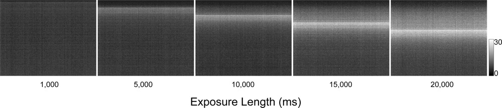
3.1.3. Progressive Shutter Band Noise

A strong horizontal band of noise occurs within all six channels of the mini-MCA, occupying approximately the same vertical position (see Figure 8). The vertical positioning of this band, its value and standard deviation are all dependent upon the exposure length (see Figure 13). Longer exposures progressively shift the band positions downwards, increasing both its value and standard deviation. Horizontal noise banding is a known artifact of CMOS sensors with progressive shutters. Despite its spatially predictable position, the increased standard deviation degrades the potential noise reduction of longer exposures. Additionally, the sharp edge of this horizontal band often generates a noticeable delineation within the corrected imagery.

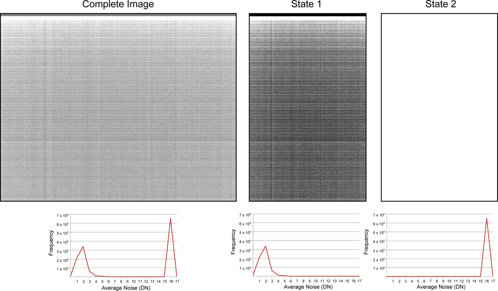
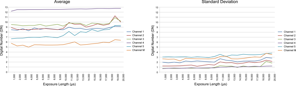
3.2. Dark Offset Potential

Figure 14 illustrates a comparative effect of dark offset subtraction across a temporal scale for the mini-MCA. The two states of each channel are condensed into a single figure for both the average and standard deviation at each exposure.

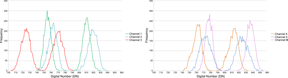
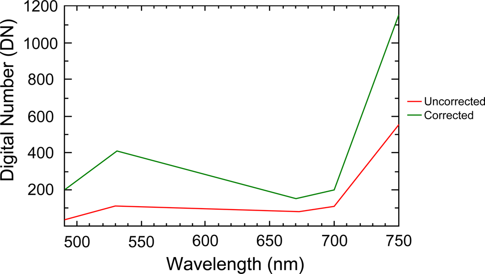
3.3. Filter Transmission/Monochromatic Efficiency
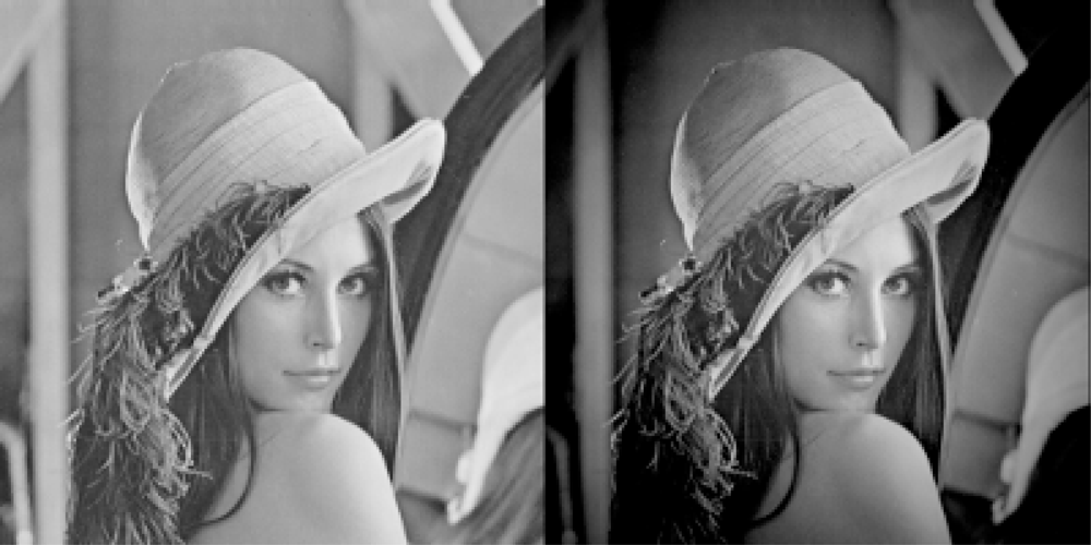
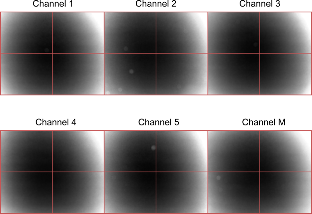
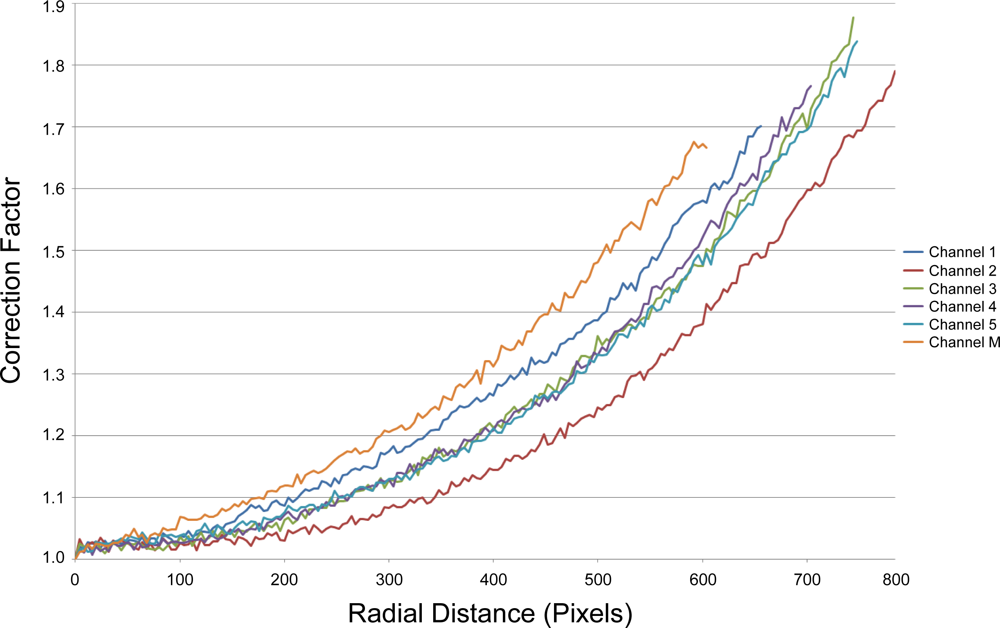
Correction factors were calculated for both filter transmission rates and relative monochromatic efficiency. A single overall correction factor was generated to account for the cumulative effects of both processes. The importance of this correction step in the restoration of interband relationships for DN data is demonstrated for a common vegetation spectral profile (see Figure 15). The effect of both processes operates only upon the radiance component of the raw data, therefore as the noise component remains unaffected, reductions in radiance directly degrade the SNR. Since application of the correction factor inflates both the radiance and noise component equally, despite the restoration of the proportional representation of the radiance component between bands, the overall SNR between differing spectral bands remains unchanged.
The six channels of the mini-MCA share a single common exposure setting. To avoid overexposure, the exposure interval must be short enough to accommodate the highest filter efficiency present across the six channels. This leaves less efficient filters suffering a relative reduction in radiance strength. Radiance reduction therefore generates a filter dependent restriction upon the available dynamic range. Dynamic range ultimately represents the precision with which data is recorded, thereby defining the smallest difference between pixels that can be detected. Reductions in dynamic range result in coarser quantisation of the data as well as degrading the SNR. Although correction factors may restore values between bands to a proportional level, both this quantisation effect and SNR remain due to the original radiance reductions set by a single exposure.

3.4. Vignetting

3.4.1. Effect of Sensors

LUT images were generated for each mini-MCA channel without filter for vignetting correction. Uniform settings were maintained between channels for comparative purpose. The vignetting structure differs between sensors both in the point of origin and in the rate of radial falloff. A visual assessment illustrates the shift in vignetting pattern origin generated by differences in the optical pathways between sensors (see Figure 16). Dust particles are evident upon the lens of Channel 2, 5 and M.
Channels additionally exhibit varying rates of vignetting radial falloff (see Figure 17). This rate of falloff is highest within channel M and lowest within channel 2. Channels 3, 4 and 5 all exhibit the most similarity in falloff rates. The variation exhibited in both origin and rate of radial falloff warrant the generation of channel specific vignetting correction LUTs.

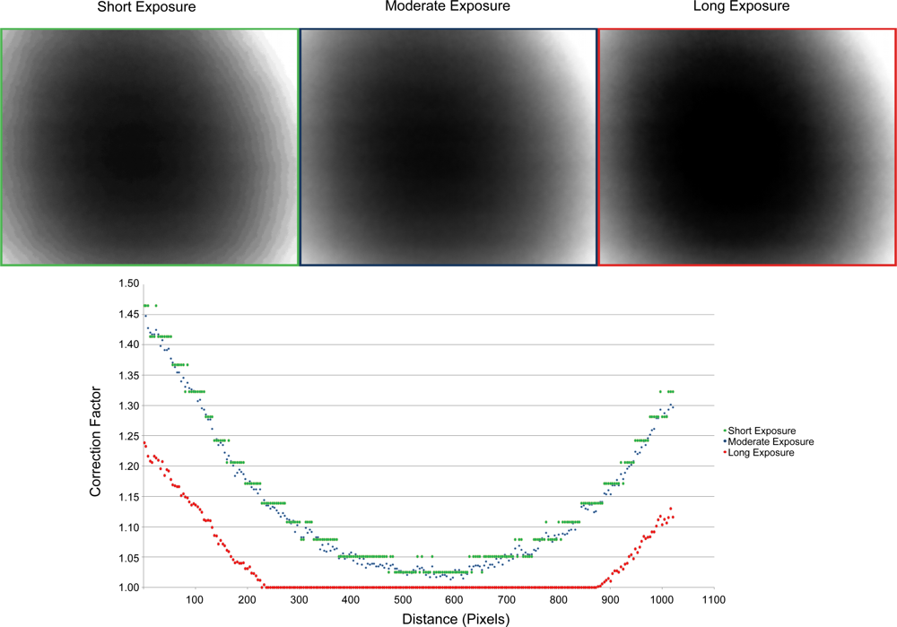
3.4.2. Effect of Exposure

Filterless LUTs were generated across a range of exposures. The LUT based approach for vignetting correction is effectively a per-pixel quantisation of the vignetting function. The degree of this quantisation is dependent upon the available dynamic range. The exposure time, therefore, ultimately determines the dynamic range of the stored flat field image. Short exposures limit the dynamic range with the subsequent quantisation generating a radial banding in the vignetting correction imagery (see Figure 18). Radial banding represents a coarser representation of illumination radial falloff. Conversely long exposures can result in saturation washing out the vignetting function. Exposure for LUT generation was balanced between maximisation in order to minimise the effects of low dynamic range in both terms of reduced SNR and the reduced smoothness of the vignetting rate of change, while avoiding the washed out effect of excessive exposure levels.
The reduction in radiance due to the effects of vignetting raises additional concerns. A reduction of radiance directly decreases the SNR and increases the coarseness of quantisation. This effect, however, is no longer uniformly global across an image, but radially dependent from the origin of vignetting. Consideration with the per-pixel SNR may necessitate the cropping of image edges if the combination of vignetting, filter transmission and monochromatic efficiency excessively degrade the SNR.

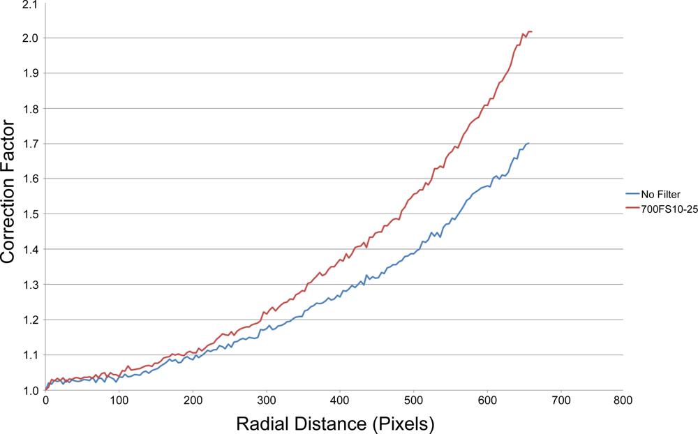
3.4.3. Effect of Filters

Filters intuitively represent a potential, additional source of mechanical vignetting. Vignetting LUTs were generated from select combinations of filters and channels. The combinations were selected based on a noise minimisation across the entire sensor. A comparison of the vignetting radial falloff reveals the effect of mounted filters. The increase in occlusion at wider angles introduced by the filter requires a corresponding increase in correction values (see Figure 19).
Vignetting LUTs and test field imagery were generated from a select combination of filter and sensor. Vignetting LUTs, generated with and without filters, were applied to the test field imagery (see Figure 20). The application of filter generated LUTs provides a noticeable improvement in vignetting correction over filterless LUTs.

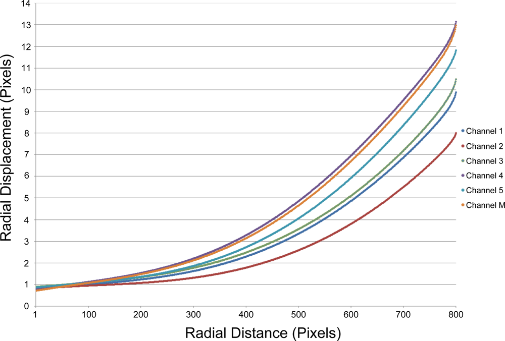
3.5. Lens Distortion

The AgiSoft Lens software package was used to calculate the distortion principal point, radial and tangential coefficients from a calibration pattern for each of the mini-MCA channels (see Table 4). Radial distortion was limited to just two coefficients as calculation of a third substantially inflates the margin of error. The AgiSoft package applies the Brown–Conrady lens distortion model, implementing both radial and tangential distortion coefficients.

Agisoft Lens Calibration Coefficients

The Brown–Conrady model using the calculated correction coefficients (Table 4) was applied to individual images. All lenses within the mini-MCA exhibit pincushion distortion (see Figure 21). The degree of lens distortion varies between sensors, with channel 5 exhibiting the strongest distortion while conversely channel M exhibits the least distortion. Lens distortion correction was applied to mini-MCA imagery (see Figure 22).

3.6. Salt Marsh Case Study

ENVI was used to convert the raw mini-MCA data into 10 bit uncorrected image bands. Corresponding image bands were identified and stacked to generate uncorrected six band multispectral imagery. A single six band multispectral salt marsh image was selected to demonstrate the effects of sensor correction. Image bands were co-registered within ENVI (rotate-scale-transform transformation). Co-registration was performed to aid in visualisation of the sensor corrections by reducing aberrations generated by differing IFOV of the sensor channels. Uncorrected true and false colour composite imagery is shown in Figure 23.
Dark offset subtraction was used to reduce the effects of noise within the imagery. Figure 24 provides an illustrative comparison of dark offset subtraction between high and low efficiency filters (750 and 490 nm respectively). Attention is drawn to the horizontal band noise strongly evident within the low efficiency filter, but masked within the high efficiency. The low efficiency filter also illustrates the limited capacity of dark offset subtraction for noise reduction.
Flat field derived LUTs were used to reduce the effects of vignetting within the salt marsh imagery. Figure 25 provides an illustrative comparison for vignetting correction. The correction demonstrates noticeable visual improvement to vegetative measurements at the periphery of the imagery, illustrating the capacity for LUTs to reduce the vignetting effect.
The effect of lens distortion correction is demonstrated by an illustrative comparison of the performance of band alignment (see Figure 26). The six mini-MCA channels all exhibit different degrees of lens distortion (see Figure 21). As the difference in distortion increases between sensor channels, it results in corresponding increase in band misalignment towards the periphery of imagery. Improving the geometric properties of the imagery through lens distortion correction improves the capacity for band alignment.
Figure 27 provides a final illustrative comparison, for both true and false colour imagery, of the combined effect of implemented sensor corrections.

4. Discussion

The phase of sensor correction serves dual roles in raw data post-processing. It is primarily an essential preliminary phase in the overall goal of extracting at-surface reflectance information from raw data. It also provides, however, the opportunity to investigate and assess data characteristics of a sensor. Such an investigation provides a practical insight into the limitations of a sensor system and the identification of potential flow-on effects of sensor idiosyncrasies.

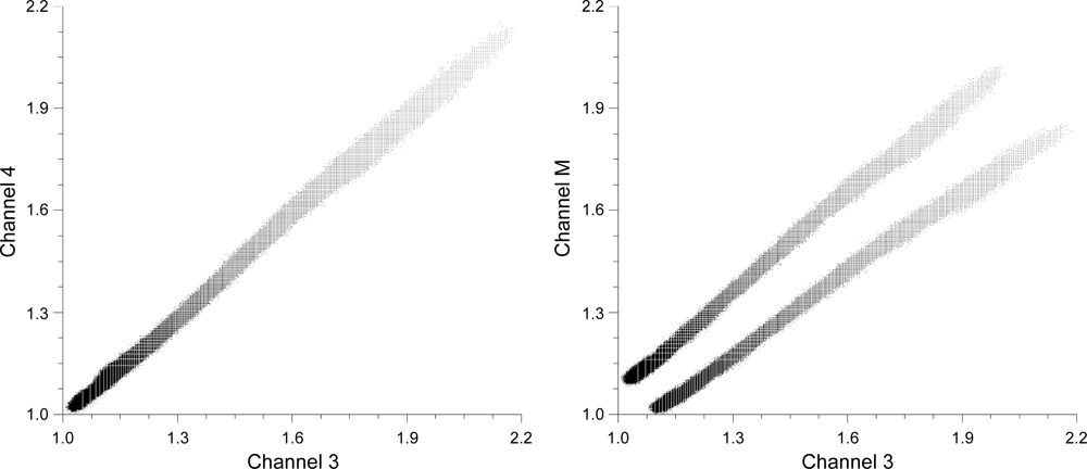
4.1. Channel Dual Distributions

It is arguable that the dual distributions effect exhibited by channels of the mini-MCA represents the strongest compromise of data quality. The exact origin of this alternating bias observed within this study remains uncertain. Regardless of its origins, the fundamental problem is the additional uncertainty generated by two distinct, yet alternating, data distributions within a single image (see Figure 28). Surfaces with similar spectral properties will exhibit dual distributions, adding strong uncertainty over the suitability of analyses based solely upon uncorrected DN values.
It is important to stress that the role of sensor correction is the extraction of DN values. Given the consistent difference between the two alternating sensor states, it becomes arguable that both states represent different, but nonetheless valid DN measurements. The stable variation exhibited between states is characteristic of recording differences that arise between different sensors.
The simplest approach for correcting this condition would be the adoption of some form of spatial averaging to reduce the differences between alternating pixels. A second option would be to adopt a dual radiometric correction/calibration approach. Although the primary role of radiometric calibration is to generate consistency between datasets, it may be forced to assume a greater role by generating consistency within datasets. As each state behaves like an individual channel, they may be treated individually during the application of radiometric calibration techniques. Calibrating for each state individually may reduce this checkered effect and improve consistency across an image.
The fundamental problem with this second approach, however, is that it is reliant upon the stable pattern of alternating distributions. Geometric corrections, particularly image mosaicing, modify the spatial properties of an image which may result in the loss of the stable alternating distributions of pixels. Therefore the application of dual radiometric calibration must be applied prior to any geometric corrections to an image.

4.2. Vignetting Model

The vignetting effect within this study was modelled through an image based flat field approach. Maximisation of the dynamic range allowed for a more smoother estimate of the per pixel falloff. An extension to this approach is the calculation of both the vignetting origin point and its rate of radial illumination falloff from the flat field, allowing for the calculation of a a smooth function [6]. This function describes the reduction in radiance striking the detector. The conversion of this radiance to a digital form, however, imparts a quantisation effect which is dependent upon the overall illumination within the scene. Such an effect becomes relevant when combinations of filters with contrasting efficiency are used, resulting in different quantisation levels. Strong quantisation may render the application of a smooth function for vignetting correction unsuitable.

4.3. Sensor Dynamic Range

UAV studies are particularly sensitive to variability in dynamic range. A major advantage of the UAV platform is the ultra high spatial resolution imagery that it can acquire. Past perspectives considered that increases in resolution would result in a corresponding increase in feature identification. This was found not to be the case, however, as the increased resolving power of finer spatial resolutions resulted in an increase in fine-scale spatial variability, thus leading to the development of more advanced image analysis techniques, including texture and object based analysis [43]. It is therefore important for UAV mounted sensors to have the necessary level of dynamic range to capture the fine-scale spatial variability inherent of ultra-high spatial resolution data.

4.4. UAV Sensor Selection

All sensors exhibit some variability in quantum efficiency across their spectrally sensitive range, in part with production quality. More expensive remote sensing platforms may opt for several individual sensors targeting specific portions of the wavelengths. Low-cost sensors, however, are inevitably forced to make concessions in production quality. The mini-MCA clearly demonstrates a flexible approach in the use of bandpass filters to select specific wavelengths. Such a flexible approach, however, requires that sensors maintain an adequate response across a wide range of wavelengths to accommodate multiple scientific purposes. Maintaining high levels of responsiveness across a wide spectral range is both technically difficult and prohibitively expensive. The resulting high variation in efficiency highlights the interplay of low-cost, flexibility, and data quality of sensor characteristics.

5. Conclusions

The mini-MCA is a low-cost, lightweight 6-channel multispectral sensor suitable for UAV remote sensing platforms. Sensor correction techniques were applied to illustrate their dual role in data quality improvement and analysis of sensor characteristics. The adoption of techniques covering noise reduction, filter transmission and relative monochromatic efficiency compensation, vignetting and lens distortion correction allowed for both improved image quality and the extraction of DN measurements. The process of sensor correction allowed for the identification of a number of issues with data collected by the mini-MCA: firstly the alternating states within a channel that result in dual noise distributions across an image, and secondly the high variability in relative monochromatic efficiency, with its associated effects upon SNR and quantisation. The dual states will require the implementation of careful post-processing techniques to generate consistency within imagery. The option to set each individual mini-MCA channel’s own unique exposure would allow for matching integration times with filter wavelength to help offset the reduction in radiance, thereby improving both SNR and quantisation level.
Sensor correction is only the first phase of post processing. DN and at-sensor radiance measurements are both limited in their applicability due to the lack of consistency with other datasets. Radiometric calibration improves consistency between datasets by reducing temporally and spatially variable environmental effects and transforming at-sensor radiance to a more universal at-surface reflectance measurement scale. Further spatial transformations include map registration, image band co-registration, and image mosaicing. Georeferencing and mosaicing is a particular important step in the creation of seamless multispectral mosaics from a large number of UAV imagery [8]. The sensor correction techniques proposed in this study should improve the results of these spatial transformation techniques due to an improved radiometric response across the individual images in a UAV survey.
Encouraged by the increased accessibility of UAVs as a remote sensing platform, small-scale in-house UAV programs will become a more commonly adopted approach for scientific endeavors. The development of these small-scale programs, however, will require a broad skillset capable of addressing all facets of UAV platform development, data post-processing, and image analysis. The adoption of low-cost UAV platforms requires the development of improved post-processing techniques in order to generate robust quantitative studies. Ultimately, the development of UAV programs necessitates a balance between accessibility (both from a technical skills and cost standpoint) with application flexibility and data quality.

Acknowledgments

We would like to acknowledge the Winifred Violet Scott Trust and the Australian Antarctic Division for financially supporting this project. We thank Darren Turner for his technical input and UAV piloting skills in the field. Finally, we would like to thank Steven de Jong for his comments on an earlier version of this manuscript.

References

  1. Zhou, G.; Ambrosia, V.; Gasiewski, A.; Bland, G. Foreword to the special issue on Unmanned Airborne Vehicle (UAV) sensing systems for earth observations. IEEE Trans. Geosci. Remote Sens 2009, 47, 687–689. [Google Scholar]
  2. Dunford, R.; Michel, K.; Gagnage, M.; Piegay, H.; Tremelo, M.L. Potential and constraints of Unmanned Aerial Vehicle technology for the characterization of Mediterranean riparian forest. Int. J. Remote Sens 2009, 30, 4915–4935. [Google Scholar]
  3. Laliberte, A.S.; Rango, A.; Herrick, J. Unmanned Aerial Vehicles for Rangeland Mapping and Monitoring : A Comparison of Two Systems. Proceedings of ASPRS Annual Conference, Tampa, FL, USA, 7–11 May 2007.
  4. Pastor, E.; Lopez, J.; Royo, P. UAV payload and mission control hardware/software architecture. IEEE Aerosp. Electron. Syst. Mag 2007, 22, 3–8. [Google Scholar]
  5. Berni, J.; Zarco-Tejada, P.; Suarez, L.; Fereres, E. Thermal and narrowband multispectral remote sensing for vegetation monitoring from an Unmanned Aerial Vehicle. IEEE Trans. Geosci. Remote Sens 2009, 47, 722–738. [Google Scholar]
  6. Lelong, C.C.D. Assessment of Unmanned Aerial Vehicles imagery for quantitative monitoring of wheat crop in small plots. Sensors 2008, 8, 3557–3585. [Google Scholar]
  7. Hunt, E.R., Jr.; Hively, W.D.; Fujikawa, S.J.; Linden, D.S.; Daughtry, C.S.T.; McCarty, G.W. Acquisition of nir-green-blue digital photographs from Unmanned Aircraft for crop monitoring. Remote Sens 2010, 2, 290–305. [Google Scholar]
  8. Laliberte, A.S.; Winters, C.; Rango, A. UAS remote sensing missions for rangeland applications. Geocarto Int 2011, 26, 141–156. [Google Scholar]
  9. Xiang, H.; Tian, L. Development of a low-cost agricultural remote sensing system based on an autonomous unmanned aerial vehicle (UAV). Biosyst. Eng 2011, 108, 174–190. [Google Scholar]
  10. Zhao, X.; Liu, J.; Tan, M. A Remote Aerial Robot for Topographic Survey. Proceedings of the 2006 IEEE/RSJ International Conference on Intelligent Robots and Systems, Beijing, China, 9–15 October 2006; pp. 3143–3148.
  11. Lin, Y.; Hyyppä, J.; Jaakkola, A. Mini-UAV-Borne LIDAR for fine-scale mapping. IEEE Geosci. Remote Sens. Lett 2011, 8, 426–430. [Google Scholar]
  12. Stefanik, K.V.; Gassaway, J.C.; Kochersberger, K.; Abbott, A.L. UAV-based stereo vision for rapid aerial terrain mapping. GISci. Remote Sens 2011, 48, 24–49. [Google Scholar]
  13. Rudol, P.; Doherty, P. Human Body Detection and Geolocalization for UAV Search and Rescue Missions Using Color and Thermal Imagery. Proceedings of the 2008 IEEE Aerospace Conference, Big Sky, MN, USA, 1–8 March 2008; pp. 1–8.
  14. Hinkley, E.A.; Zajkowski, T. USDA forest serviceNASA: Unmanned aerial systems demonstrations pushing the leading edge in fire mapping. Geocarto Int 2011, 26, 103–111. [Google Scholar]
  15. Pastor, E.; Barrado, C.; Royo, P.; Santamaria, E.; Lopez, J.; Salami, E. Architecture for a helicopter-based unmanned aerial systems wildfire surveillance system. Geocarto Int 2011, 26, 113–131. [Google Scholar]
  16. Walter, M.; Niethammer, U.; Rothmund, S.; Joswig, M. Joint analysis of the Super-Sauze (French Alps) mudslide by nanoseismic monitoring and UAV-based remote sensing. EGU Gen. Assem 2009, 27, 53–60. [Google Scholar]
  17. Laliberte, A.; Goforth, M.; Steele, C.; Rango, A. Multispectral remote sensing from unmanned aircraft: image processing workflows and applications for rangeland environments. Remote Sens 2011, 3, 2529–2551. [Google Scholar]
  18. Clodius, W.B.; Weber, P.G.; Borel, C.C.; Smith, B.W. Multi-spectral band selection for satellite-based systems. Proc. SPIE 1998, 3377, 11–21. [Google Scholar]
  19. Glenn, E.P.; Huete, A.R.; Nagler, P.L.; Nelson, S.G. Relationship between remotely-sensed vegetation indices, canopy attributes and plant physiological processes: What vegetation indices can and cannot tell us about the landscape. Sensors 2008, 8, 2136–2160. [Google Scholar]
  20. Lacava, T.; Brocca, L.; Calice, G.; Melone, F.; Moramarco, T.; Pergola, N.; Tramutoli, V. Soil moisture variations monitoring by AMSU-based soil wetness indices: A long-term inter-comparison with ground measurements. Remote Sens. Environ 2010, 114, 2317–2325. [Google Scholar]
  21. Asner, G.P. Biophysical and biochemical sources of variability in canopy reflectance. Remote Sens. Environ 1998, 64, 234–253. [Google Scholar]
  22. Smith, M.; Edward, J.; Milton, G. The use of the empirical line method to calibrate remotely sensed data to reflectance. Int. J. Remote Sens 1999, 20, 2653–2662. [Google Scholar]
  23. Mahiny, A.S.; Turner, B.J. A comparison of four common atmospheric correction methods. Photogramm. Eng. Remote Sensing 2007, 73, 361–368. [Google Scholar]
  24. Cooley, T.; Anderson, G.; Felde, G.; Hoke, M.; Ratkowski, A.J.; Chetwynd, J.; Gardner, J.; Adler-Golden, S.; Matthew, M.; Berk, A.; et al. FLAASH, A MODTRAN4-Based Atmospheric Correction Algorithm, Its Application and Validation. Proceedings of the IEEE International Geoscience Remote Sensing Symposium, Toronto, ON, Canada, 24–28 June 2002; 3, pp. 1414–1418.
  25. Al-amri, S.S.; Kalyankar, N.V.; Khamitkar, S.D. A comparative study of removal noise from remote sensing image. J. Comput. Sci 2010, 7, 32–36. [Google Scholar]
  26. Mansouri, A.; Marzani, F.; Gouton, P. Development of a protocol for CCD calibration: Application to a multispectral imaging system. Int. J. Robot. Autom 2005, 20. [Google Scholar] [CrossRef]
  27. Chi, C.; Zhang, J.; Liu, Z. Study on methods of noise reduction in a stripped image. Int. Arch. Photogramm. Remote Sens. Spat. Inf. Sci 2008, 37, Part 6B. 213–216. [Google Scholar]
  28. Mullikin, J.C. Methods for CCD camera characterization. Proc. SPIE 1994, 2173, 73–84. [Google Scholar]
  29. Goldman, D.B. Vignette and exposure calibration and compensation. IEEE Trans. Pattern Anal. Mach. Intell 2010, 32, 2276–2288. [Google Scholar]
  30. Kim, S.J.; Pollefeys, M. Robust radiometric calibration and vignetting correction. IEEE Trans. Pattern Anal. Mach. Intell 2008, 30, 562–576. [Google Scholar]
  31. Zheng, Y.; Lin, S.; Kambhamettu, C.; Yu, J.; Kang, S.B. Single-image vignetting correction. IEEE Trans. Pattern Anal. Mach. Intell 2009, 31, 2243–2256. [Google Scholar]
  32. Yu, W. Practical anti-vignetting methods for digital cameras. IEEE Trans. Consum. Electron 2004, 50, 975–983. [Google Scholar]
  33. Wang, A.; Qiu, T.; Shao, L. A simple method of radial distortion correction with centre of distortion estimation. J. Math. Imag. Vis 2009, 35, 165–172. [Google Scholar]
  34. Prescott, B. Line-based correction of radial lens distortion. Graph. Model. Image Process 1997, 59, 39–47. [Google Scholar]
  35. Hugemann, W. Correcting Lens Distortions in Digital Photographs; Ingenieurbüro Morawski + Hugemann: Leverkusen, Germany, 2010. [Google Scholar]
  36. Park, J.; Byun, S.C.; Lee, B.U. Lens distortion correction using ideal image coordinates. IEEE Trans. Consum. Electron 2009, 55, 987–991. [Google Scholar]
  37. Jedlička, J.; Potčková, M. Correction of Radial Distortion in Digital Images; Charles University in Prague: Prague, Czech, 2006. [Google Scholar]
  38. de Villiers, J.P.; Leuschner, F.W.; Geldenhuys, R. Modeling of radial asymmetry in lens distortion facilitated by modern optimization techniques. Proc. SPIE 2010, 7539, 75390J:1–75390J:8. [Google Scholar]
  39. Wang, J.; Shi, F.; Zhang, J.; Liu, Y. A New Calibration Model and Method of Camera Lens Distortion. Proceedings of 2006 IEEE/RSJ Int. Conf. Intell. Robot. Syst., Beijing, China, 9–15 October 2006; pp. 5713–5718.
  40. Adam, P. Saltmarshes in a time of change. Environ. Conserv 2002, 29, 39–61. [Google Scholar]
  41. Emery, N.C.; Ewanchuk, P.J.; Bertness, M.D. Competition and salt-marsh plant zonation: Stress tolerators may be dominant competitors. Ecology 2001, 82, 2471–2485. [Google Scholar]
  42. Pennings, S.C.; Callaway, R.M. Salt marsh plant zonation: The relative importance of competition and physical factors. Ecology 1992, 73, 681–690. [Google Scholar]
  43. Puissant, A.; Hirsch, J.; Weber, C. The utility of texture analysis to improve per-pixel classification for high to very high spatial resolution imagery. Int. J. Remote Sens 2005, 26, 733–745. [Google Scholar]
Figure 1. Comparative imagery of saltmarsh captured at different scales with different platforms: satellite, UAV, field (satellite imagery: GoogleEarth).
Remotesensing 04 01462f1
Figure 2. Modified Tetracam Miniature Multiple Camera Array (Mini-MCA).
Remotesensing 04 01462f2
Figure 3. Image data pre-processing: Sensor correction and radiometric calibration.
Remotesensing 04 01462f3
Figure 4. Illustration of the effects of increased noise proportion: Original image, 5 % noise, 25 % noise
Remotesensing 04 01462f4
Figure 5. Relative Monochromatic Response and Absolute Filter Transmission.
Remotesensing 04 01462f5
Figure 6. Illustration of the effects of vignetting: Original image, image exhibiting the radial shadowing of vignetting.
Remotesensing 04 01462f6
Figure 7. Forms of lens distortion: original, barrel lens distortion, pincushion lens distortion.
Remotesensing 04 01462f7
Figure 8. Dark offset imagery from the six channels of the mini-MCA: single sample, average of 125 samples, standard deviation of 125 samples.
Remotesensing 04 01462f8aRemotesensing 04 01462f8b
Figure 9. Distribution of noise within dark offset imagery for all six channels of the mini-MCA (Exposure 1,000 μs).
Remotesensing 04 01462f9
Figure 10. Separation of bimodal condition within Channel 2 of the mini-MCA (Exposure 1,000 μs).
Remotesensing 04 01462f10
Figure 11. Flat field subsample illustrating pronounced bimodal condition within each channel.
Remotesensing 04 01462f11
Figure 12. Illustration of the limited capacity for periodic structure removal with dark offset subtraction.
Remotesensing 04 01462f12
Figure 13. Illustration of the temporal progression of shutter band noise present within all channels of the mini-MCA.
Remotesensing 04 01462f13
Figure 14. Response of noise response to lengthening exposure: average, standard deviation.
Remotesensing 04 01462f14
Figure 15. Effect of corrective factor upon vegetation spectral profile.
Remotesensing 04 01462f15
Figure 16. Vignetting LUTs generated from all six channels of the mini-MCA.
Remotesensing 04 01462f16
Figure 17. Vignetting radial falloff for all six sensors of the mini-MCA.
Remotesensing 04 01462f17
Figure 18. Effect of exposure on quantisation, and subsequent effect upon the vignetting radial falloff.
Remotesensing 04 01462f18
Figure 19. Comparison of the rate of vignetting radial falloff in the presence/absence of a filter.
Remotesensing 04 01462f19
Figure 20. Application of vignetting correction : Original uncorrected image, application of filterless LUTs, application of Filter LUTs.
Remotesensing 04 01462f20
Figure 21. Radial distortion of all six channels within the mini-MCA.
Remotesensing 04 01462f21
Figure 22. Illustrative lens distortion map of channel 3 of the mini-MCA.
Remotesensing 04 01462f22
Figure 23. Uncorrected true and false colour composite mini-MCA imagery.
Remotesensing 04 01462f23
Figure 24. Comparative dark offset performance between high and low efficiency filters.
Remotesensing 04 01462f24
Figure 25. Comparative dark offset performance between high and low efficiency filters.
Remotesensing 04 01462f25
Figure 26. Comparative band alignment illustrating subtle improvement due to lens distortion correction.
Remotesensing 04 01462f26
Figure 27. Comparative true and false colour composites before and after sensor corrections.
Remotesensing 04 01462f27
Figure 28. Checkered condition within the mini-MCA giving rise to multiple radiance distributions.
Remotesensing 04 01462f28
Table 1. Filter Transmission/Monochromatic efficiency Correction Factors.
Filter (nm)Transmission (%)Correction FactorMonochromatic Relative Efficiency (%)Correction FactorMultiplicative Correction Factor
4500.442.280.166.2514.27
4900.472.130.342.976.32
5300.472.120.561.803.81
5500.452.210.621.613.57
5700.442.260.671.493.38
6700.561.800.911.101.98
7000.561.790.931.081.92
7200.511.960.951.052.06
7500.492.020.971.032.09
9000.482.070.711.402.90
9700.472.140.452.224.75
Table 2. Image Acquisition Details.
DateSiteLongitudeLatitudeHeight (m)Exposure (μs)
25/11/2012Ralphs Bay42 55.742′S147 29.036′E100 m4,000
Table 3. Sensor Noise Characteristics.
ChannelStateAverageStDevSkew
118.4450.650−3.379
28.4520.6817−2.987
211.8280.8841.559
215.9720.670−23.798
316.9990.317−18.182
211.9810.504−23.543
419.3740.626−5.627
214.9740.628−23.801
517.7570.542−5.664
25.5270.747−1.094
M18.0200.449−10.784
23.5080.7621.247
Table 4. Lens Distortion Coefficients.
Channelcxcyk1k2p1p2FxFy
1629.169465.738−0.0687450.0623006−0.000639335−0.0005098791622.51622.5
2628.961464.003−0.05796490.0356426−0.000102067−0.002214391606.811606.81
3632.575472.777−0.05066970.0214840.0000776870.00113171625.741625.74
4633.999470.756−0.09124270.132531−0.0001350510.001240681623.551623.55
5632.498470.568−0.07486130.07293010.000851022−0.0003999021625.881625.88
M638.965460.592−0.09221080.1241070.0006144660.0008422891619.261619.26

