A MODIS-Based Energy Balance to Estimate Evapotranspiration for Clear-Sky Days in Brazilian Tropical Savannas

 ,
,
Abstract
:1. Introduction
2. Methodology
2.1. Surface Energy Balance Algorithm for Land
2.1.1. Model Description
2.1.2. Remote Sensing Input Data
2.2. The Hydrological Model MGB-IPH
2.2.1. Model Description
2.2.2. Input Data and Model Validation
- pasture, grassland and cropland areas with soils of medium storage capacity (HRU 1);
- cropland areas with soils of high storage capacity (HRU 2);
- soils with low storage capacity (HRU 3);
- forest and reforested areas on soils with medium storage capacity (HRU 4);
- pasture, grassland and bare soil on soils with high storage capacity (HRU 5);
- open water surfaces (HRU 6).
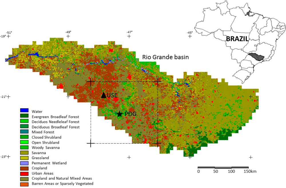
2.3. Site Description
2.4. Study Area
2.5. Data Analysis
3. Results and Discussions
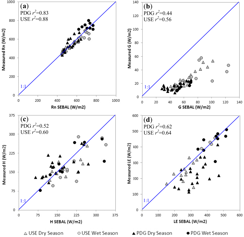
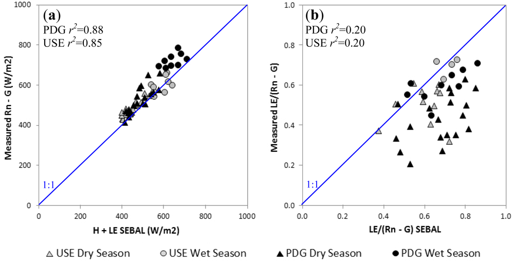
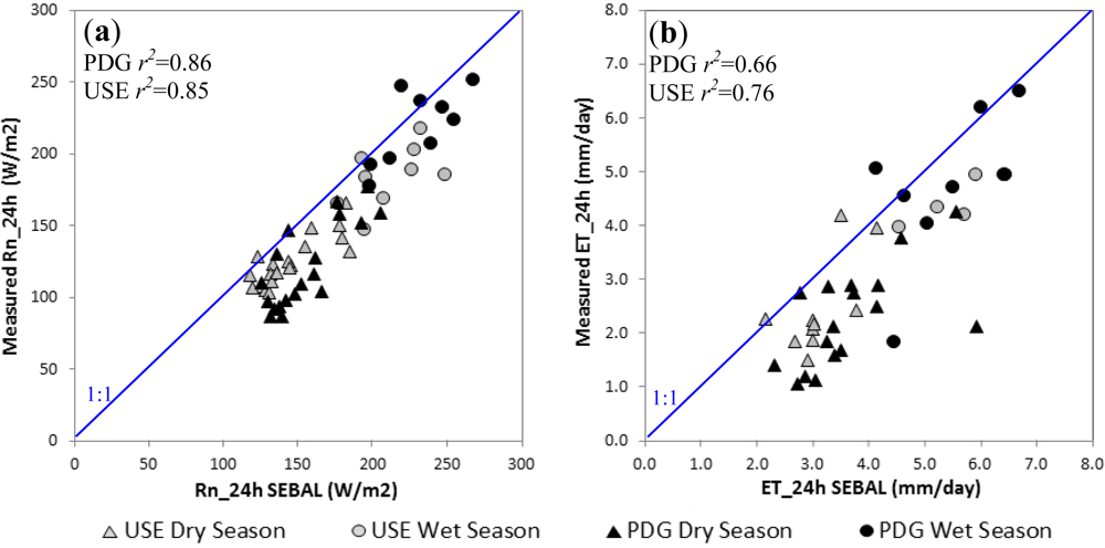
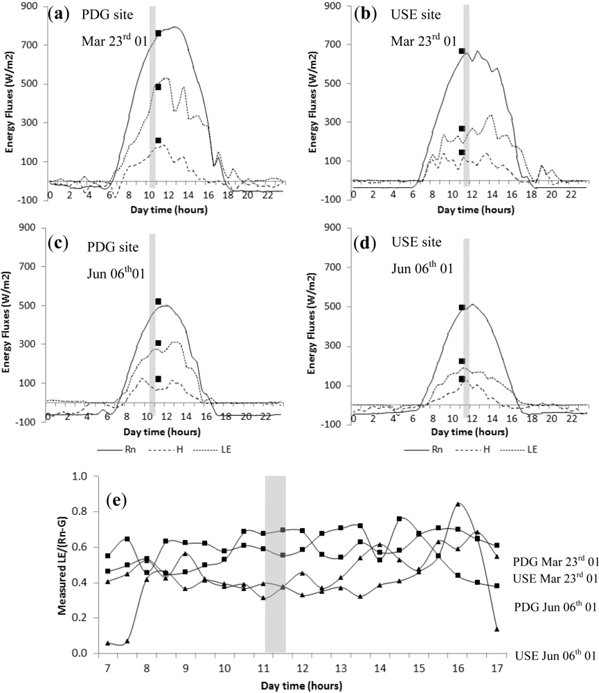
3.1. Validation of SEBAL’s Instantaneous Energy Fluxes
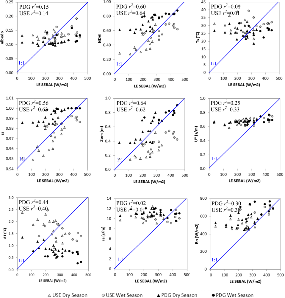
3.2. Control of SEBAL’s Instantaneous Latent Heat Flux
3.3. Scaling SEBAL’s Instantaneous Latent Heat Flux to Daily Evapotranspiration
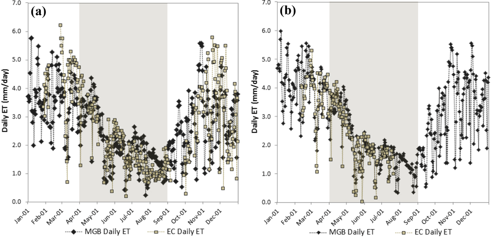
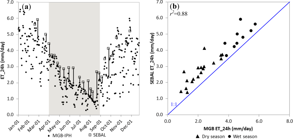
3.4. Estimation of Daily Evapotranspiration by Hydrological Modelling
3.5. Evapotranspiration at Basin Scale
4. Concluding Remarks
- The omission of a soil moisture constraint for a region of known water limitations.
- The description of vegetation water stress by NDVI, which is limited by the asymptotic saturation level in areas where biomass index is high and information about vegetation water content is difficult to obtain.
- The subjective determination of the gradient of temperature (dT) to estimate sensible heat fluxes (H).
- Limitations from the compensatory or cumulative errors entered through the residual energy balance, partitioning turbulent fluxes and estimating EF and Rn,24h.
- The omission of night net radiation (Rn) when it becomes effectively negative or even assuming that average daily soil heat flux (G) is zero can lead to overestimations.
Acknowledgments
References
- Allen, R.G.; Tasumi, M.; Trezza, R. Satellite-Based Energy Balance for Mapping Evapotranspiration with Internalized Calibration (METRIC)—Model. J. Irrig. Drain. Eng 2007, 133, 380–394. [Google Scholar]
- Norman, J.M.; Anderson, M.C.; Kustas, W.P.; French, A.N.; Mecikalski, J.; Torn, R.; Diak, G.R.; Schmugge, T.J.; Tanner, B.C.W. Remote sensing of surface energy fluxes at 101m pixel resolutions. Water Resour. Res 2003, 39, 1221–1229. [Google Scholar]
- Su, Z. The Surface Energy Balance System (SEBS) for estimation of turbulent heat fluxes. Hydrol. Earth Syst. Sci 2002, 6, 85–99. [Google Scholar]
- Roerink, G.J.; Su, Z.; Menenti, M. S-SEBI: A simple remote sensing algorithm to estimate the surface energy balance. Phys. Chem. Earth Pt B 2000, 25, 147–157. [Google Scholar]
- Bastiaanssen, W.G.M.; Menenti, M.; Feddes, R.A.; Holtslag, A.M. A remote sensing surface energy balance algorithm for land (SEBAL). 1. Formulation. J. Hydrol 1998, 212–213, 198–212. [Google Scholar]
- Bastiaanssen, W.G.M.; Pelgrum, H.; Wang, J.; Ma, Y.; Moreno, J.F.; Roerink, G.J.; Van der Tal, T. A remote sensing surface energy balance algorithm for land (SEBAL). 2. Validation. J. Hydrol 1998, 212–213, 213–229. [Google Scholar]
- Norman, J.M.; Kustas, W.; Humes, K. A two-source approach for estimating soil and vegetation energy fluxes from observations of directional radiometric surface temperature. Agr. For. Meteorol 1995, 77, 263–293. [Google Scholar]
- Kalma, J.D.; Jupp, D.L.B. Estimating evaporation from pasture using infrared thermometry: evaluation of a one-layer resistance model. Agr. For. Meteorol 1990, 51, 223–246. [Google Scholar]
- Zwart, S.J.; Bastiaanssen, W.G.M. SEBAL for detecting spatial variation of water productivity and scope for improvement in eight irrigated wheat systems. Agr. Water Manage 2007, 89, 287–296. [Google Scholar]
- Hemakumara, H.M.; Chandrapala, L.; Moene, A.F. Evapotranspiration fluxes over mixed vegetation areas measured from large aperture scintillometer. Agr. Water Manage 2003, 58, 109–122. [Google Scholar]
- Allen, R.G.; Tasumi, M.; Trezza, R.; Waters, R.; Bastiaanssen, WG.M. Surface Energy Balance Algorithm for Land (SEBAL)—Advanced Training and User’s Manual; University of Idaho: Kimberly, ID, USA, 2002; p. 98. [Google Scholar]
- Lagouarde, J.P.; Jacob, F.; Gu, X.F.; Olioso, A.; Bonnefond, J.M.; Kerr, Y.; Mcaneney, K.J.; Irvine, M. Spazialization of sensible heat flux over a heterogeneous landscape. Agronomie 2002, 22, 627–633. [Google Scholar]
- Bastiaanssen, W.G.M. SEBAL-based sensible and latent heat fluxes in the irrigated Gediz Basin, Turkey. J. Hydrol 2000, 229, 87–100. [Google Scholar]
- Kite, G.W.; Drogers, P. Comparing evapotranspiration estimates from satellites, hydrological models and field data. J. Hydrol 2000, 229, 3–18. [Google Scholar]
- Wang, J.; Ma, Y.; Menenti, M.; Bastiaanssen, W.G.M.; Mistsuta, Y. The scaling-up of processes in the heterogeneous landscape of HEIFE with the aid of satellite remote sensing. J. Meteor. Soc. Jpn 1995, 73, 1235–1244. [Google Scholar]
- French, A.N.; Jacob, F.; Anderson, M.C.; Kustas, W.P.; Timmermans, W.; Gieske, A.; Su, Z.; Su, H.; McCabe, M.F.; Li, F.; Prueger, J.; Brunsell, N. Surface energy fluxes with the advanced Spaceborne Thermal Emissions and Reflectation Radiometer (ASTER) at the Iowa 2002 SMACEX site (USA). Remote Sens. Environ 2005, 99, 55–65. [Google Scholar]
- Jacob, F.; Olioso, A.; Gu, X.; Su, Z.; Seguin, B. Mapping surface fluxes using airborne visible, near infrared, thermal infrared remote sensing and a spatialized surface energy balance model. Agronomie 2002, 22, 669–680. [Google Scholar]
- Vinukollu, R.K.; Wood, E.F.; Ferguson, C.R.; Fisher, J.B. Global estimates of evapotranspiration for climate studies using multi-sensor remote sensing data: Evaluation of three process-based approaches. Remote Sens. Environ 2011, 115, 801–823. [Google Scholar]
- Lauer, D.T.; Morain, S.A.; Salomonson, V.V. The Landsat Program: its origins, evolution, and impacts. Photogramm. Eng. Remote Sensing 1997, 63, 831–838. [Google Scholar]
- Carmel, Y. Controlling data uncertainty via aggregation in remotely sensed data. IEEE Geosci. Remote Sens. Lett 2004, 1, 39–41. [Google Scholar]
- Van Rompaey, A.J.J.; Govers, G.; Baudet, M. A strategy for controlling error of distributed environmental models by aggregation. Int. J. GIS 1999, 13, 577–590. [Google Scholar]
- Dai, X.L.; Khorram, S. The effects of image misregistration on the accuracy of remotely sensed change detection. IEEE Trans. Geosci. Remote Sens 1998, 36, 1566–1577. [Google Scholar]
- Carmel, Y.; Dean, J.; Flather, C.H. Combining location and classification error sources of estimating multi-temporal database accuracy. Photogramm. Eng. Remote Sensing 2001, 67, 865–872. [Google Scholar]
- Gupta, V.K.; Rodriguez-Iturbe, I.; Wood, E.F. Scale Problems in Hydrology; Reidel Publishing Company: Dordrecht, The Netherlands, 1986; p. 260. [Google Scholar]
- Mu, Q.; Zhao, M.; Running, S.W. Improvements to a MODIS Global Terrestrial Evapotranspiration Algorithm. Remote Sens. Environ 2011, 115, 1781–1800. [Google Scholar]
- Mallick, K.; Bhattacharya, B.K.; Rao, V.U.M.; Reddy, D.R.; Banerjee, S.; Hoshali, V.; Pandey, V.; Kar, G.; Mukherjee, J.; Vyas, S.P.; Gadgil, A.S.; Patel, N.K. Latent heat flux estimation in clear sky days over Indian agroecosystems using noontime satellite remote sensing data. Agr. For. Meteorol 2009, 149, 1646–1665. [Google Scholar]
- Venturini, V.; Islam, S.; Rodriguez, L. Estimation of evaporative fraction and evapotranspiration from MODIS products using a complementary based model. Remote Sens. Environ 2008, 112, 132–141. [Google Scholar]
- Cleugh, H.A.; Leuning, R.; Mu, Q.; Running, S.W. Regional evaporation estimates from flux tower and MODIS satellite data. Remote Sens. Environ 2007, 106, 285–304. [Google Scholar]
- Mu, Q.; Heinsch, F.A.; Zhao, M.; Running, S.W. Development of a global evapotranspiration algorithm based on MODIS and global meteorology data. Remote Sens. Environ 2007, 111, 519–536. [Google Scholar]
- Batra, N.; Islam, S.; Venturini, V.; Bisht, G.; Jiang, L. Estimation and comparison of evapotranspiration from MODIS and AVHRR sensors for clear sky days over the Southern Great Plains. Remote Sens. Environ 2006, 103, 1–15. [Google Scholar]
- Nishida, K.; Nemani, R.R.; Running, S.W.; Glassy, J.M. An operational remote sensing algorithm for land surface evaporation. J. Geophys. Res 2003, 108, 4270–4283. [Google Scholar]
- Nishida, K.; Nemani, R.R.; Running, S.W.; Glassy, J.M. Development of an evapotranspiration index from Aqua/MODIS for monitoring surface moisture status. IEEE Trans. Geosci. Remote Sens 2003, 41, 493–501. [Google Scholar]
- Collischonn, W.; Allasia, D.; Silva, B.C.; Tucci, C.E.M. The MGB-IPH model for large scale rainfall runoff modeling. Hydrol. Sci. J 2007, 52, 878–895. [Google Scholar]
- Tasumi, M.; Trezza, R.; Allen, R.G.; Wright, J.L. Operational aspects of satellite-based energy balance models for irrigated crops in the semi-arid US. J. Hydrol. Eng 2008, 19, 355–376. [Google Scholar]
- Van de Griend, A.A.; Owe, M. On the relationship between thermal emissivity and normalized difference vegetation index for natural surfaces. Int. J. Remote Sens 1993, 14, 1119–1131. [Google Scholar]
- Crago, R.D. Conservation and variability of the evaporative fraction during the daytime. J. Hydrol 1996, 180, 173–194. [Google Scholar]
- Bisht, G.; Venturini, V.; Islam, S.; Jiang, L. Estimation of the net radiation using MODIS (Moderate Resolution Imaging Spectroradiometer) data for clear sky days. Remote Sens. Environ 2005, 97, 52–67. [Google Scholar]
- Brutsaert, W. Hydrology: An Introduction; Cambridge University Press: London, UK, 2005; p. 618. [Google Scholar]
- Vermote, E.F.; Kotchenova, S.Y.; Ray, J.P. MODIS Surface Reflectance User’s Guide. 2010. Available online: http://modis-sr.ltdri.org/products/MOD09_UserGuide_v1_2.pdf (accessed on 23 November 2010).
- Wan, Z. MODIS Land Surface Temperature Products Users’ Guide. 2010. Available online: http://www.icess.ucsb.edu/modis/LstUsrGuide/MODIS_LST_products_Users_guide_C5.pdf (accessed on 23 November 2010).
- Solano, R.; Didan, K.; Jacobson, A.; Huete, A. MODIS Vegetation Indices (MOD13) C5 User’s Guide. 2010. Available online: http://tbrs.arizona.edu/project/MODIS/UsersGuide.pdf (accessed on 23 November 2010).
- Wan, Z.; Li, Z.L. Radiance - based validation of the V5 MODIS land - surface temperature product. Int. J. Remote Sens 2008, 29, 5373–5395. [Google Scholar]
- Huete, A.; Justice, C.O.; Van Leeuwen, W. MODIS Vegetation Index (MOD13): Algorithm Theoretical Basis Document. 2011. Available online: http://modis.gsfc.nasa.gov/data/atbd/atbd_mod13.pdf (accessed on 8 February 2011).
- Paz, A.R.; Collischonn, W. River reach length and slope estimates for large-scale hydrological models based on a relatively high-resolution digital elevation model. J. Hydrol 2007, 343, 127–139. [Google Scholar]
- Beven, K. How far can we go in distributed hydrological modelling? Hydrol. Earth Syst. Sci 2001, 5, 1–12. [Google Scholar]
- Kouwen, N.; Soulis, E.; Pietroniro, A.; Donald, J.; Harrington, R. Grouped response units for distributed hydrologic modeling. J. Water Res. Pl-ASCE 1993, 119, 289–305. [Google Scholar]
- Monteith, J.L. Evaporation and Environment. In The State and Movement of Water in Living Organism; Fogg, B.D., Ed.; Symposium of the Society of Experimental Biology XIX: Cambridge, UK, 1965; pp. 205–234. [Google Scholar]
- Wigmosta, M.S.; Vail, L.W.; Lettenmaier, D.P. A distributed hydrology-vegetation model for complex terrain. Water Resour. Res 1994, 30, 1665–1679. [Google Scholar]
- Shuttleworth, W.J. Evaporation. In Handbook of Hydrology; Maidment, D.R., Ed.; McGRaw Hill: New York, NY, USA, 1993; pp. 4.1–4.53. [Google Scholar]
- Nóbrega, M.T.; Collischonn, W.; Tucci, C.E.M.; Paz, A.R. Uncertainty in climate change impacts on water resources in the Rio Grande Basin, Brazil. Hydrol. Earth Syst. Sci 2011, 15, 585–595. [Google Scholar]
- Getirana, A.C.V.; Bonnet, M.P.; Rotunno-Filho, O.C.; Collischonn, W.; Guyot, J.L.; Seyler, F.; Mansur, W.J. Hydrological modelling and water balance of the Negro River basin: evaluation based on in situ and spatial altimetry data. Hydrol. Process 2010, 24, 3219–3236. [Google Scholar]
- Collischonn, W.; Silva, B.C.; Tucci, C.E.M.; Allasia, D.G. Large basin simulation experience in South America. IAHS Pub 2006, 303, 360–370. [Google Scholar]
- Collischonn, W.; Tucci, C.E.M.; Haas, R.; Andreolli, I. Forecasting river Uruguay flow using rainfall forecasts from a regional weather-prediction model. J. Hydrol 2005, 305, 87–98. [Google Scholar]
- Agência Nacional de Águas. HidroWeb—Sistema de Informações Hidrológicas. Available online: http://hidroweb.ana.gov.br/ (accessed on 23 November 2010).
- Coordenadoria de Recursos Hídricos do Estado de São Paulo. Sistema Integrado de Gerenciamento de Recursos Hídricos do Estado de São Paulo. Available online: http://www.sigrh.sp.gov.br/ (accessed on 23 November 2010).
- Centro de Previsão do Tempo e Estudos Climáticos. Plataformas de coleta de dados. Available online: http://satelite.cptec.inpe.br/PCD/ (accessed on 23 November 2010).
- Ministério das Minas e Energia. Projeto RADAM Brasil. Brasília, Brazil. Available online: http://www.projeto.radam.nom.br/ (accessed on 23 November 2010).
- Collischonn, W.; Tucci, C.E.M.; Clarke, R.T. Previsão de Afluência a Reservatórios Hidrelétricos: Módulo 1; Universidade Federal do Rio Grande do Sul: Porto Alegre, Brazil, 2007; p. 188. [Google Scholar]
- Tucci, C.E.M.; Collischonn, W.; Clarke, R.T.; Paz, A.R.; Allasia, D. Short and long-term flow forecasting in the Rio Grande watershed (Brazil). Atmos. Sci. Lett 2008, 9, 53–56. [Google Scholar]
- Juárez, R.I.N. Variabilidade climática regional e controle da vegetação no sudeste: Um estudo de observações sobre cerrado e cana-de-açúcar e modelagem numérica da atmosfera. PhD Thesis, Universidade de São Paulo, São Paulo, Brazil. 2004; 185. [Google Scholar]
- Cabral, O.M.R.; Rocha, H.R.; Ligo, M.A.; Brunini, O.; Dias, M.A.F.S. Fluxos turbulentos de calor sensível, vapor d’água e CO2 sobre plantação de cana-de-açúcar (saccharum sp) em Sertãozinho, SP. Rev. Bras. Meteorol 2003, 18, 61–70. [Google Scholar]
- Rocha, H.R.; Freitas, H.C.; Dias, M.A.F.S.; Ligo, M.A.; Cabral, O.M.R.; Tannus, R.N.; Rosolem, R. Measurements of CO2 exchange over a woodland savanna (Cerrado sensu stricto) in southeast Brasil. Biota Neotrop 2002, 2, 1–11. [Google Scholar]
- Ferguson, C.R.; Wood, E.F.; Sheffield, J.; Gao, H. Quantifying uncertainty in a remote sensing-based estimate of evapotranspiration over continental USA. Int. J. Remote Sens 2010, 31, 3821–3865. [Google Scholar]
- Anderson, M.; Norman, J.; Diak, G.; Kustas, W.P.; Mecikalski, J.R. A two-source time integrated model for estimating surface fluxes using thermal infrared remote sensing. Remote Sens. Environ 1997, 60, 195–216. [Google Scholar]
- Kustas, W.P.; Humes, K.; Norman, J.M.; Moran, M. Single and dual source modeling of surface energy fluxes with radiometric surface temperature. J. Appl. Meteorol 1996, 35, 110–121. [Google Scholar]
- Zhan, X.; Kustas, W.P.; Humes, K. An intercomparison study on models of sensible heat flux over partial canopy surfaces with remotely sensed surface temperature. Remote Sens. Environ 1996, 58, 242–256. [Google Scholar]
- Teixeira, A.H.C. Determining regional actual evapotranspiration of irrigated crops and natural vegetation in the São Francisco River Basin (Brazil) using remote sensing and Penman-Monteith Equation. Remote Sens 2010, 2, 1287–1319. [Google Scholar]
- Alexandridis, T.K.; Cherif, I.; Chemin, Y.; Silleos, G.N.; Stavrinos, E.; Zalidis, G.C. Integrated methodology for estimating water use in Mediterranean agricultural areas. Remote Sens 2009, 1, 445–465. [Google Scholar]
- Foken, T. The energy balance closure problem: An overview. Ecol. Appl 2008, 18, 1351–1367. [Google Scholar]
- Culf, A.D.; Foken, T.; Gash, J.H.C. The Energy Balance Closure Problem. In Vegetation, Water, Humans and the Climate: A New Perspective on an Interactive System; Kabat, P., Claussen, M., Dirmeyer, P.A., Gash, J.H.C., Bravo, D.E., Guenni, L., Meybeck, M., Pielke, R., Vörösmarty, C.J., Hutjes, R.W.A., Lütkemeier, S, Eds.; Springer: Berlim, Germany, 2004; pp. 159–166. [Google Scholar]
- Wilson, K.; Goldstein, A.; Falge, E.; Aubinet, M.; Baldocchi, D.D.; Berbigier, P.; Bernhofer, C.; Ceulemans, R.; Dolman, H.; Field, C.; et al. Energy balance closure at FLUXNET sites. Agr. For. Meteorol 2002, 113, 223–243. [Google Scholar]
- Huete, A.; Didan, K.; Miura, T.; Rodriguez, E.P.; Gao, X.; Ferreira, L.G. Overview of the radiometric and biophysical performance of the MODIS vegetation indices. Remote Sens. Environ 2002, 83, 195–213. [Google Scholar]
- Aragão, L.E.O.C.; Shimabukuro, Y.E.; Santo, F.B.E.; Williams, M. Spatial validation of collection 4 MODISLAI product in eastern amazon. IEEE Trans. Geosci. Remote Sens 2005, 43, 2526–2534. [Google Scholar]
- Sellers, P.J. Canopy reflectance, photosynthesis and transpiration. Int. J. Remote Sens 1985, 6, 1335–1372. [Google Scholar]
- Cecatto, P.; Gobron, N.; Flasse, S.; Pinty, B.; Tarantola, S. Designing a spectral index to estimate vegetation water content from remote sensing data: Part 1: Theoretical approach. Remote Sens. Environ 2002, 82, 188–197. [Google Scholar]
- Tucker, C.J. Remote sensing of leaf water content in the near infrared. Remote Sens. Environ 1980, 10, 23–32. [Google Scholar]
- Gao, B.C. NDWI—A normalized difference water index for remote sensing of vegetation liquid water from space. Remote Sens. Environ 1996, 58, 257–266. [Google Scholar]
- Gu, Y.; Brown, J.F.; Verdin, J.P.; Wardlow, B. A five-year analysis of MODIS NDVI and NDWI for grassland drought assessment over the central Great Plains of the United States. Geophys. Res. Lett 2007, 34, L06407. [Google Scholar]
- Delbart, N.; Kergoat, L.; Toan, T.L.; Lhermitte, J.; Picard, G. Determination of phenological dates in boreal regions using normalized difference water index. Remote Sens. Environ 2005, 97, 26–38. [Google Scholar]
- Jackson, J.T.; Chen, D.; Cosh, M.; Li, F.; Anderson, M.; Walthall, C.; Doriaswamy, P.; Hunt, E.R. Vegetation water content mapping using Landsat data derived normalized difference water index for corn and soybeans. Remote Sens. Environ 2004, 92, 475–482. [Google Scholar]
- Allen, R.G.; Tasumi, M.; Morse, A.; Trezza, R. A Landsat-based energy balance and evapotranspiration model in Western US water rights regulation and planning. Irrig. Drain. Syst 2005, 19, 251–268. [Google Scholar]
- Fisher, J.B.; Baldocchi, D.D.; Misson, L.; Dawson, T.E.; Goldstein, A.H. What the towers don’t see at night: nocturnal sap flow in trees and shrubs at two AmeriFlux sites in California. Tree Physiol 2007, 27, 597–610. [Google Scholar]
- McCabe, M.F.; Wood, E.F. Scale influences on the remote estimation of evapotranspiration using multiple satellite sensors. Remote Sens. Environ 2006, 105, 271–285. [Google Scholar]
- Wan, Z.; Zhang, Y.; Zhang, Q.; Li, Z.L. Quality assessment and validation of the MODIS global land surface temperature. Int. J. Remote Sens 2004, 25, 261–274. [Google Scholar]
- Wan, Z.; Zhang, Y.; Zhang, Q.; Li, Z.L. Validation of the land-surface temperature products retrieved from Terra Moderate Resolution Imaging Spectroradiometer data. Remote Sens. Environ 2002, 83, 163–180. [Google Scholar]


| HRU 1 | HRU 2 | HRU 4 | HRU 5 | ||
|---|---|---|---|---|---|
| Area (Km2) | 8,510 | 13,686 | 6,085 | 9,364 | |
| r2 | 0.86 (p < 0.05) | 0.65 (p < 0.05) | 0.46 (p < 0.05) | 0.79 (p < 0.05) | |
| MAE (mm day−1) | 1.2 | 0.4 | 0.9 | 0.7 | |
| RMSE (mm·day−1) | 1.2 | 0.7 | 1.1 | 0.9 | |
| Avg±StDev (mm day−1) | MGB-IPH | 2.4 ± 1.7 | 2.6 ± 1.3 | 2.8 ± 1.2 | 2.5 ± 1.5 |
| SEBAL | 3.7 ± 1.2 | 3.1 ± 1.2 | 3.7 ± 1.2 | 3.3 ± 1.2 | |
Share and Cite
Ruhoff, A.L.; Paz, A.R.; Collischonn, W.; Aragao, L.E.O.C.; Rocha, H.R.; Malhi, Y.S. A MODIS-Based Energy Balance to Estimate Evapotranspiration for Clear-Sky Days in Brazilian Tropical Savannas. Remote Sens. 2012, 4, 703-725. https://doi.org/10.3390/rs4030703
Ruhoff AL, Paz AR, Collischonn W, Aragao LEOC, Rocha HR, Malhi YS. A MODIS-Based Energy Balance to Estimate Evapotranspiration for Clear-Sky Days in Brazilian Tropical Savannas. Remote Sensing. 2012; 4(3):703-725. https://doi.org/10.3390/rs4030703
Chicago/Turabian StyleRuhoff, Anderson L., Adriano R. Paz, Walter Collischonn, Luiz E.O.C. Aragao, Humberto R. Rocha, and Yadvinder S. Malhi. 2012. "A MODIS-Based Energy Balance to Estimate Evapotranspiration for Clear-Sky Days in Brazilian Tropical Savannas" Remote Sensing 4, no. 3: 703-725. https://doi.org/10.3390/rs4030703