Article

Estimating the Maximal Light Use Efficiency for Different Vegetation through the CASA Model Combined with Time-Series Remote Sensing Data and Ground Measurements

1
Institute of Mountain Hazards and Environment, Chinese Academy of Sciences, Chengdu 610041, China
2
Department of Geography, University of Maryland, College Park, MD 20742, USA
*
Author to whom correspondence should be addressed.
Remote Sens. 2012, 4(12), 3857-3876; https://doi.org/10.3390/rs4123857
Submission received: 29 September 2012 / Revised: 21 November 2012 / Accepted: 22 November 2012 / Published: 5 December 2012

Abstract

:
Maximal light use efficiency (LUE) is an important ecological index of a vegetation essential attribute, and a key parameter of the LUE-based model for estimating large-scale vegetation productivity by remote sensing technology. However, although currently used in different models there still exists extensive controversy. This paper takes the Zoige Plateau in China as a case area to develop a new approach for estimating the maximal LUEs for different vegetation. Based on an existing land cover map and MODIS NDVI product, the linear unmixing method with a moving window was adopted to estimate the time-series NDVI for different end members in a MODIS NDVI pixel; then Particle Swarm Optimizer (PSO) was applied to search for the optimization of LUE retrievals through the CASA (Carnegie-Ames-Stanford Approach) model combined with time-series NDVI and ground measurements. The derived maximal LUEs present significant differences among various vegetation types. These are 0.669 gC·MJ−1, 0.450 gC·MJ−1 and 0.126 gC·MJ−1 for the xerophilous grasslands with high, moderate and low vegetation fraction respectively, 0.192 gC·MJ−1 for the hygrophilous grasslands, and 0.125 gC·MJ−1 for the helobious grasslands. The field validation shows that the estimated net primary productivity (NPP) by the derived maximal LUE is closely related to the ground references, with R2 of 0.8698 and root-mean-square error (RMSE) of 59.37 gC·m−2·a−1. This indicates that the default set in the CASA model is not suitable for NPP estimation for the regional mountain area. The derived maximal LUEs can significantly improve the capability of NPP mapping, and open up the perspective for long-term monitoring of vegetation ecological health and ecosystem productivity by combining the LUE-based model with remote sensing observations.

1. Introduction

Light use efficiency (LUE) is an index that describes the efficiency of vegetation for fixing solar energy [1]. It is a key parameter of LUE-based models for modeling the vegetation productivity at regional to global scales [25], and is considered a constant, rather than a variable for certain vegetation types or even entire eco-regions. However, the maximal LUE currently used in these models still gives rise to extensive controversy [6], especially in the mountain area which is normally covered by high heterogeneous vegetation. Estimating the maximal LUE of vegetation is of great significance for mapping the NPP and diagnosing the long-time vegetation health conditions, and to further assist both relevant management and policy-making for protecting the ecological environment.
Maximal LUE is an essential attribute of plants [7], however, at different scales, the comprehensive influences of plant physiological factors, species composition, climate and environment factors, may cause the LUE to show obvious spatial heterogeneity [8]. The maximal LUE of vegetation is mainly related to the chlorophyll content, species, leaf age, light intensity, and growth stages at the leaf scale. While at the canopy scale, many factors such as leaf area index (LAI), leaf inclination angle, solar zenith angle, observation angle and canopy structure may influence the LUE [9]. When applying remote-sensed data to estimate NPP at the regional scale, the differences of LUEs among dissimilar vegetation types cannot be ignored [10,11]. Similarly, at the global scale, according to the modeling results by coupling atmospheric CO2 observation, satellite remote-sensing and atmospheric radiation transfer models, it has been observed that with the maximal LUE of vegetation there also exists obvious geographical differences [12]. Methods of acquiring maximal LUE include the biomass survey method [13], the light quantum efficiency reckoning method [14], the eddy covariance technology reckoning method [15], and the productivity model inversion method [16], etc. A lot of previous research studied LUE difference through site-based measurements [1719]. While in-situ measurements, especially on complex terrain surface, introduced significant bias when scaling up to a large spatial size [6,20]. In recent years, some progress has been made using the photochemical reflectance index [2124]. However, the high sensitivity of this index to various extraneous effects such as canopy structure and view observer geometry has so far prevented its use at landscape scales [24].
Deriving the maximal LUE through LUE-based models is an effective alternative, and has been extensively applied because of its simple mechanism, fewer required physiological and ecological parameters, and easy combination with the remote-sensing data [10,11]. The satellite remotely sensed data has a relatively continuous sequence in time and space, and the Normalized Difference Vegetation Index (NDVI), a spectral index linearly related to the fraction of the photosynthetically active radiation (400–700 nm) intercepted by the canopy [25], has proven to be a proxy for the status of the aboveground biomass at the landscape level. It is usually applied as the key input parameter for driving the LUE model, such as the CASA model, in which NDVI is used to compute the light absorption proportion of vegetation [26]. However, when retrieving the LUE through the CASA model, the effect of the pixels mixed by different vegetation types increases the uncertainty [27], and it is most obviously shown in moderate- and low-resolution spatial resolution images, such as the time-series NDVI products of MODIS [28].
Over years, researchers have explored the spectral imaging mechanisms and the spectral mixing process, and have developed various unmixing methods such as the linear unmixing method [29], the probability unmixing method [30], the geometric optics unmixing method [29], and the random geometric unmixing method [29], etc. However, unmixing of mixed pixels in previous works is mostly based on the spectral reflectivity of various bands of multi-spectral images, and the number of bands is generally required to be more than the number of endmember components. Such methods are normally faced with the limitation for determining endmembers. The time-series NDVI unmixing is a method for decreasing the spatial dimension with temporal information. The main idea of it is to unmix the time-series NDVI of mixed pixels into the time-series NDVI of some specific land-cover components [31], which can integrate the time phase information of multi-temporal images to derive the time-series NDVI of different endmember components, and finally reduce spectral information variation brought about by mixed pixels.
In this paper, taking the grassland-wetland ecosystems on the Zoige Plateau in China as a case, we attempt to propose an approach for directly estimating the maximal LUE for different vegetation types based on the CASA model through spectral unmixing analysis of time-series NDVI combined with ground measurements. The specific objectives of this paper are to (1) explore whether unmixing of time-series NDVI can improve the accuracy of maximal LUE inversion and (2) identify whether there is significant difference among the maximal LUE of different vegetation types at the landscape level.

2. Material and Methods
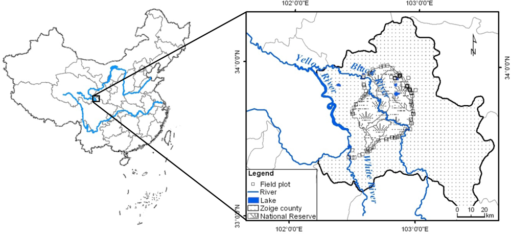
2.1. Study Area

The Zoige Plateau is located at the eastern edge of the Tibetan Plateau in China, with typical character of both mountain and plateau. It is the largest alpine peat swamp area in the world [32,33], and also a water conservation area of the upper reaches of the Yangtze River and the Yellow River (Figure 1). Several national natural reserves have been established in this area to serve as functions for ecological conservation [34]. This paper takes the administrative Zoige county as a case area which is a core and typical region on the Zoige Plateau (Figure 1). The study area is mainly covered by herbaceous vegetation including alpine meadow and aquatic plants with obvious ecological vulnerability. In recent years, the desertification of grasslands and the shrinking of wetlands have become more and more serious, directly due to the influence of human activities such as excessive grazing, and land reclamation through digging drainage for the wetlands [35].
Weather in the Zoige Plateau is cold and relatively wet, with an annual mean temperature of 0.7 °C to 3.3 °C [32]. Due to good atmospheric transparency, radiation on the Plateau is very strong, and the diurnal range of air temperature is large, with a range of 15 °C to 16 °C. The phenophase of hrebaceous plants in this area varies significantly for different vegetation types. The growing period is roughly divided into five sections: turning green (26 March to 16 April), leaf expansion (2–16 May), stem extension (30 June to 16 July), blossom (14 July to 27 July), grain filling and maturation (8–24 August) [36]. Because of the complex vegetation community on the Zoige Plateau, it is representative and suitable for the study of LUE spatial variability at the landscape scale.

2.2. Data and Processing

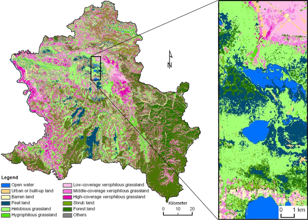
2.2.1. Remote Sensing Data

This study applies the MODIS MOD13Q1 NDVI product with a spatial resolution of 250 m as the basic remote sensing data. It is derived by the 16-day Maximum Value Composite (MVC) method [37], and thus contains 23 temporal NDVI images in a year. The product in 2009 is collected from the data access URL: https://lpdaac.usgs.gov/lpdaac/products/modis_products_table. Because the study area is located at the Plateau which is characterized by a lot of cloud, ice or snow cover, the time-series NDVI product is reconstructed by the Savitzky-Golay filter to reduce noise and improve data quality for subsequent analysis. For the data process method refer to our previous publications [3840]. One scene of a Landsat-5 image acquired in a clear sky condition on 28 July 2009 (path/row: 130/37) was collected from the International Scientific Data Service Platform ( http://datamirror.csdb.cn/). It was applied as the reference for validating the unmixing results of MODIS time-series NDVI. The acquisition date is around the blossom period of grasses on the Zoige Plateau. The preprocess software developed by the LEDAPS program [41] was adopted to acquire the surface reflectance, which is then used to calculate the NDVI of TM.
An existing land cover map with the spatial resolution of 30 m (Figure 2) is also used to calculate the fractional cover of each endmember in the pixels of MODIS NDVI. It is derived from TM images and auxiliary data such as DEM and time-series NDVI by the matter-element fuzzy decision-making classifier, with an overall precision of 89.89% [42]. The grassland vegetation is classified into five cover types including hygrophilous grass, helobious grass, high-coverage xerophilous grass, middle-coverage xerophilous grass, and low-coverage xerophilous grass. Helobious grasslands are located in shallow water or moisture saturated soil, where dominant plant communities include marsh plants and aquatic plants such as Carex-like plants, Potamogeton-like plants, Utricularia-like plants, Phragmites, etc. Hygrophilous grasslands are distributed widely on the Zoige plateau, and grow mainly in moist soil conditions. Their dominant plant communities include Kobresia-like plants, Carex-like plants, Parnassia-like plants, Poa pratensis-like plants, etc., with a relatively low fragmentation (Figure 2). Xerophilous grasslands are the widest distributed grass cover in this area. Their dominant plant communities include Kobresia-like plants, Potentilla-like plants, Elymus-like plants, Deyeuxia-like plants, Festuca-like plants, Leontopodium-like plants, Ranunculus-like plants and so on [43]. Low-, middle- and high coverage defined here is coverage of 5–20 percent, 20–50 percent and more than 50 percent respectively.

2.2.2. The Meteorological Observations

The meteorological data used here include precipitation, average air velocity, average atmospheric pressure, average temperature, relative humidity, minimum temperature, maximum temperature, sunshine hours, and solar radiation, which are provided by the Meteorological Information Center of the China Meteorological Administration. These observations need to be rescaled to the 16-day composited data from daily observations, so as to match the temporal scale of MODIS NDVI. There are more than 700 meteorological observation stations in China, while just 122 of them supply solar radiation data, and there is no radiation station located inside the study area. Zhang [44] once pointed out that the downward radiation of a ground-based observation can just represent the area of no more than 10 km2 in the plain area. Using site-based observations to substitute or interpolate contiguous surface radiation l causes great errors. In this paper, combining the meteorological observation station network with DEM data, we applied an optimized Ångström-Prescott model [45,46] to model the global solar radiation at the rugged area. The derived contiguous global solar radiation on the Zoige Plateau was validated by situ-measurement, and the accuracy reached 81.66 percent (Figure 3). The relevant study will be reported in another paper.

2.2.3. The Ground Measurements

The growing season of plants on the Zoige Plateau lasts from May to August. The grasses usually accumulate the maximum biomass and then wither around mid-September. The field sampling measurements were conducted in September 2009. A total of 56 sample plots (with an approximate sampling distance more than 1,000 m) were harvested according to the regional random sampling theory [47] and the stratified sampling method. The size of a sample plot is designed as 100 m × 100 m. Most sample plots are located at a relative flat surface covered with a single vegetation type with an area more than 500 × 500 m2. Such sampling design can ensure a sample plot to cover at least one complete MODIS pixel. The spatial distribution of the sample plots is shown in Figure 1. In each sample plot, we randomly selected six quadrats with a size of 1 × 1 m2, and harvested the aboveground grass in the quadrats. The harvest biomass is first dried and then converted into NPP by an empirical coefficient of 0.475 [48,49], which means about 47.5 percent NPP will be sequestrated into the aboveground biomass. The average value of the six quadrats is assigned to the sample plot. The statistics of field-measured NPPs are listed in Table 1.

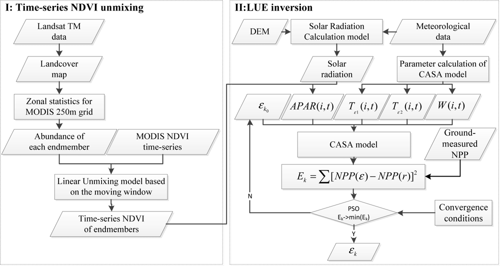
2.3. Model Development

The overall approach is algorithmically divided into two parts: the time-series NDVI unmixing and the LUE inversion. The overall flowchart is designed as shown in Figure 4. Combining with an existing land cover map with a 30 m spatial resolution (Figure 2), we adopt a time-series unmixing method with a moving window to reconstruct the time-series NDVI of each endmember. The LUE inversion models are then established to invert the maximal LUEs for different vegetation types. The process includes deriving the input parameters of the CASA model and setting an objective function for the LUE inversion. The Particle Swarm Optimization (PSO) method is used to search for the optimum solution until the objective function meets the convergence conditions.

2.3.1. The Time-Series NDVI Unmixing

In some earlier studies e.g., [50,51], it was supposed that the time-series NDVI of a mixed pixel was the linear combination of different vegetation components in that pixel. Combined with a given land cover map, the NDVI of each endmember can be estimated by the linear unmixing method. The time-series NDVI of a mixed pixel can be expressed as follows [28]:
NDVI ( i , t ) = c = 1 k ( fc ( i , c ) × NDVI ¯ i ( c , t ) ) + e ( i , t )
c = 1 k ( fc ( i , c ) = 1
where NDVI(i,t) is the NDVI value at time t of the ith pixel, fc(i,c) is the area ratio of the cth vegetation in the ith pixel, NDVI ¯ i ( c , t ) is the NDVI mean value at time t of vegetation cover c in the ith pixel, k is the number of vegetation types in the ith pixel and e(i,t) is the residual error of NDVI linear combination of pixel i.
The linear unmixing method needs to meet the assumption that spectral properties of a land cover type do not show great variations [52]. Therefore, this study uses a moving window in the time-series NDVI unmixing. The window size should satisfy two conditions: (1) the window size should be small enough to meet the above assumption and (2) the window should contain sufficient mixed pixels to construct an over determined linear function. Based on the heterogeneity of land cover types, the window with size of 5 × 5 pixels is determined. The unmixing of time-series NDVI of N pixels in a moving window then can be expressed in the following linear equation set:
[ NDVI ( 1 , t ) NDVI ( i , t ) NDVI ( N , t ) ] = [ fc ( 1 , 1 ) fc ( 1 , c ) fc ( 1 , K ) fc ( i , 1 ) fc ( i , c ) fc ( i , K ) fc ( N , 1 ) fc ( N , c ) fc ( N , K ) ] [ NDVI ¯ ( 1 , t ) ) NDVI ¯ ( c , t ) ) NDVI ¯ ( K , t ) ) ] + [ e ( 1 , t ) ) e ( i , t ) ) e ( N , t ) ) ]
where NDVI(i,t) is the NDVI value at time t of the ith MODIS pixel within the 5 × 5 window, N is equal to 25, fc(i,c) is the area ratio of the cth vegetation in the ith pixel, which is aggregated from the land-cover map with a resolution of 30 m into 250 m. The other parameters are the same as the ones in Equation (1).

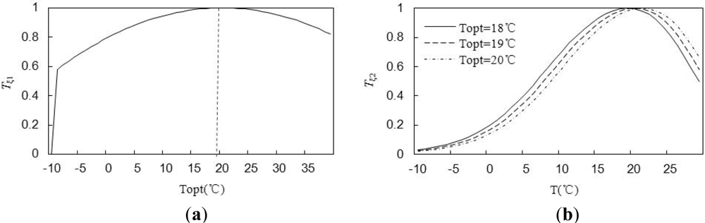
2.3.2. Derivation of the Input Parameters for the CASA Model

The CASA model is a typical light use efficiency model that integrates the vegetation intrinsic attributes with the environmental conditions [26,53]. In this model, NPP can be expressed as a function of the absorbed photosynthetically active radiation (APAR) by vegetation and actual LUE (ε) [26]:
NPP ( x , t ) = APAR ( x , t ) × ε ( x , t )
And, the APAR (x, t) can be calculated by:
APAR ( x , t ) = SOL ( x , t ) × FPAR ( x , t ) × 0.5
where SOL(x,t) refers to the global solar radiation of pixel x during the time t, and FPAR(x,t) is the fraction of Photosynthetically Active Radiation (PAR) absorbed by the plant canopy. Within a certain range, linear relations exist between FPAR and NDVI, which can be determined by the maximum and minimum values of NDVI of certain vegetation types together with the corresponding maximum and minimum values of FRAR:
FPAR ( x , t ) = ( NDVI ( x , t ) NDVI i , min ) ( NDVI i , max NDVI i , min ) × ( FPAR max FPAR min ) + FPAR min
where NDVIi,max and NDVIi,min correspond respectively to the maximum and minimum values of NDVI of the ith vegetation cover. The input data NDVI(x,t) in Equation (6) is the output result of the time-series NDVI unmixing.
In ideal conditions, vegetation has the maximal LUE. However, the LUE under real conditions is always influenced by temperature and moisture. Their relationship can be expressed as:
ε ( x , t ) = T ε 1 ( x , t ) × T ε 2 ( x , t ) × W ε ( x , t ) × ε max
where εmax is the maximal LUE, and the default set of εmax in the CASA model (ε0) is assigned to a constant value of 0.389 gC·MJ−1, Tε1(x,t) and Tε2(x,t) represent the stress effects of temperature upon the LUE, and Wε(x,t) is the water stress influence coefficient. For the detailed equations and models for calculating the parameters of temperature and moisture stress refer to the relevant literature [26,54,55].

2.3.3. Objective Function of the LUEs Inversion

Combined with the CASA model, the objective function for assessing the error of model-derived NPP is designed as follows:
E k = j = 1 n k ( NPP ( ε ) j NPP ( r ) j ) 2
where Ek represents the squared error between the ground-measured NPP(r) and the CASA model-derived NPP(ε) for the kth endmember, nk represents the numbers of field sample plots of the kth endmember. NPP(ε) can be considered as a function of the priori maximal LUE(ε), NDVI of endmembers, and model-required meteorological observations (Equations (47)).
When Ek reaches the minimum value, the output εk is the optimum maximal LUE of each endmember. The function can be express as:
ε k = ε ( E k min ( E k ) )
where the convergence conditions of Equation (9) are designed as: Ek less than 5 or the maximum iteration times less than 2,000.
The Particle Swarm Optimizer (PSO) is used to search for the global optimum solution of Equation (9). The PSO is a population-based stochastic optimization technique developed by Kennedy and Eberhart [56], inspired by social behavior of bird flocking. Compared with genetic algorithms, all the particles tend to converge to the best solution quickly even in the local version, in most cases.

2.3.4. Model Assessment

The derived models are evaluated using cross-validation, a technique for deriving relatively independent accuracy estimates when only limited reference samples are available for model development [57]. A four-fold cross-validation method is used to validate the prediction of the derived maximal LUE through the CASA model for “unknown data”. The NPP of field samples are divided into four subsets. Three of the subsets are used as training datasets to estimate the maximal LUE through Equation (9), and the remaining one is used to test the model-derived NPP by Equation (4) using the estimated maximal LUE. The testing procedure is carried out four times until every subset has been tested. Model performance is measured by the agreement between the modeling results and the actual field measurements. For each model, we calculate a R2 value and a root mean square of the difference (RMSE) following standard statistical textbooks.

3. Results and Analysis

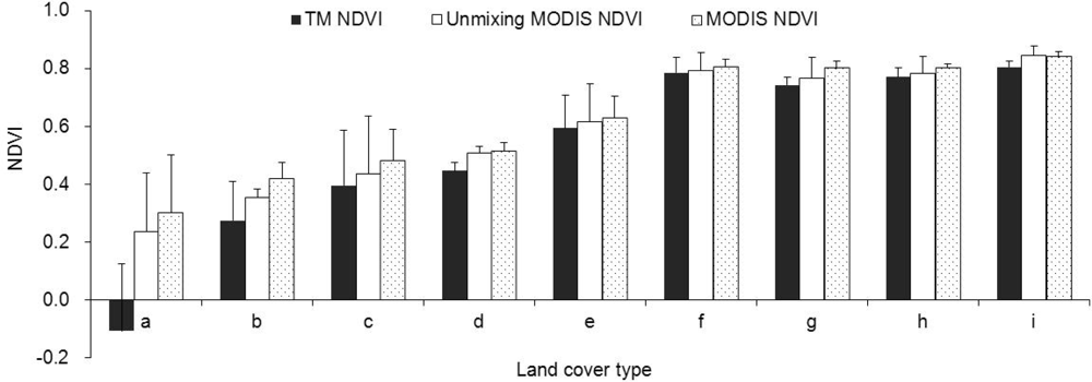
3.1. Unmixing of the Time-Series NDVI

The unmixing of the time-series NDVI has varying degrees of improvement for different land covers. In Figure 5, TM NDVI is taken as the reference to validate the unmixing results of time-series NDVI. Comparing to the original MODIS product, the mean NDVIs of unmixing results are closer to those of TM data for most land covers. This indicates that time-series unmixing can improve the NDVI accuracy. NDVI of helobious grassland is the lowest among the grassland covers, which indicates that helobious grassland has relatively low greenness. The unmixing gives NDVI of helobious grassland 3.96 percent lower than its original value of MODIS. For hygrophilous grasslands, the difference of NDVI between TM and MODIS is small and the unmixing only makes the NDVI 1.6 percent lower than its original value of MODIS. Meanwhile, the unmixing causes 4.04 and 2.24 percent decrease of the original NDVI of MODIS respectively for low- and middle-coverage xerophilous grasslands. High-coverage xerophilous grasslands are more contiguous (Figure 2) and their high coverage can decrease the impact of background. As a result, the unmixing process presents no obvious improvement for high-coverage xerophilous grasslands.
Among the non-vegetation covers, NDVI of open water is the lowest, and the difference between TM and MODIS is the largest. The mean NDVI of open water is −0.107 in TM while 0.458 in MODIS. The land cover map shows the open water is often mixed with the vegetation cover or peat land, simultaneously, the same results are also obviously found in urban or built-up land and barren land (Figure 2). The urban area of Zoige county is approximate 2.3 km2, which just covers about 37 pixels in MODIS; the barren land scatters and mainly distributes in the bealock and windward slopes, or along the ancient riverbed. It results from grassland degeneration and desertification that is caused by overgrazing or marsh drainage [58]. Comparing to TM images, more pixels of MODIS images in urban or barren land area are combined with grasslands, and NDVI of those pixels are impacted by the surrounding land covers. As a result, the unmixing has improved the NDVI quality for barren land and building land (Figure 5). Peat land distributes widely on the Zoige Plateau. It is the largest concentrated area of plateau peat swamp in the world, and mainly concentrates in the river terrace or the surrounding of lakes or the low-lying areas (Figure 2), with the low degree of fragmentation [32]. As a result, there is no significant change on the NDVI unmixing for peat land.

3.2. The Derived Maximal LUEs

According to the time-series NDVI unmixing results, FPAR and APAR of each vegetation cover are calculated through the Equations (5) and (6). Using the meteorological data and field measurements, the maximal LUEs of different vegetation are derived through CASA model combined with the optimizing objective Equation (8). Since the number of field sample plots is limited, a four-fold cross-validation is used to test the inversion results. Table 2 shows the derived maximal LUE of different vegetation covers without and with time-series unmixing in the study area.
Without the time-series unmixing, the estimated maximal LUEs of high-coverage xerophilous and moderate-coverage xerophilous grassland are 0.669 gC·MJ−1 with variation range of 0.652–0.696 gC·MJ−1, and 0.450 gC·MJ−1 with variation range of 0.440–0.452 gC·MJ−1 respectively (Table 2). They are both higher than the original set in the CASA model (0.389 gC·MJ−1). The optimal estimated maximal LUE of low-coverage grassland, hygrophilous grassland and helobious grassland are 0.126 gC·MJ−1, 0.192 gC·MJ−1 and 0.125 gC·MJ−1 respectively (Table 2), and all lower than the default in the CASA model. Simultaneously, Table 2 shows that the inversion results of LUEs from the NDVI unmixing of each endmember are relative higher than the results estimated by the original MODIS NDVI, especially for high-coverage grassland. A similar result is also found in previous literature [7,11], which implies that it likely be the consequence of different spatial scales.
Peng et al.[59] and Zhu et al.[60] reported that the maximal LUE used in the CASA model might be different from the default set for different vegetations in China, which can also be strongly supported by the findings of this paper. From the results, the maximal LUEs of high-coverage and moderate-coverage xerophilous grassland are similar to those in the study of Running et al.[50] (the maximal LUE of grassland is 0.608 gC·MJ−1). The maximal LUEs of hygrophilous and helobious grasslands as well as their simulated NPPs are both relatively low (Table 2), which is consistent with the field-measured biomass. Nevertheless, researches of LUE on hygrophilous and helobious grasslands have not been seen so far in the literature.

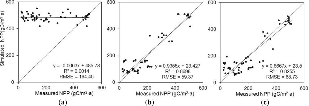
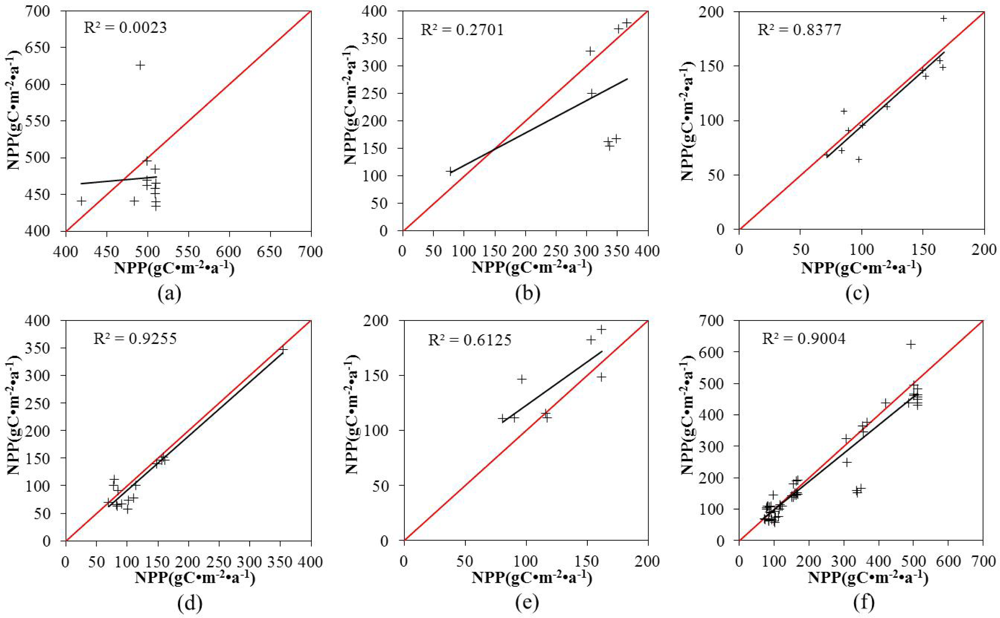
3.3. Accuracy Evaluation

To evaluate the accuracy of the derived maximal LUE, the default set of the CASA model, the derived maximal LUEs with and without the time-series NDVI unmixing are separately utilized to estimate the NPPs for different vegetation covers. As shown in Figure 6(a), using the single default set of the CASA model, the simulated NPPs of sample plots differ greatly from the field measurements, with R2 of about 0.0014 and RMSE of 164.45 gC·m−2·a−1. The model-derived NPPs for all vegetation types are in the range of 418.81–550.59 gC·m−2·a−1, and cannot reflect the spatial heterogeneity of vegetation cover on the Zoige Plateau. However, using the optimization of maximal LUEs for different vegetation cover, the consistence between the model-simulated NPP and the field-measured NPP is improved significantly with R2 of 0.8698 and the RMSE of 59.37 gC·m−2·a−1 (Figure 6(b)). This indicates that the derived maximal LUEs are better than the default set in the original CASA model which is normally used to estimate NPP at the global scale. Although Table 2 shows that the time-series NDVI unmixing affects the results of LUEs inversion, the unmixing has no improvement for NPP estimation compared with the method without the time-series NDVI unmixing, with R2 of 0.8255 and the RMSE of 68.73 gC·m−2·a−1 (Figure 6(c)).
On the whole, the simulated NPPs with NDVI unmixing are lower than those without NDVI unmixing (Figure 7(f)), although the unmixing increases the value of derived LUEs (Table 2). Figure 5 shows that unmixing decreases the value of NDVI, and makes it closer to the NDVI of TM. Because FAPAR has a positive linear relationship with NDVI [61,62], FAPAR and APAR will also decrease along with NDVI. According to the Equations (46), the simulated results of NPP reflect the unmixing results of NDVI. This implies that the derived NPPs by the LUE-based model and remotely sensed NDVI are more sensitive to NDVI than to the maximal LUE. The analysis also further verifies that, as well as calibrating the maximal LUEs for different vegetation cover, the unmixing of time-series NDVI or obtaining NDVI with higher spatial resolution is very important for regional NPP mapping. However, the unmixing method used in this paper also shows the different consequences for NPP estimation for different vegetation cover. Middle-coverage xerophilous grassland (Figure 7(b)), Low-coverage xerophilous grassland (Figure 7(c)) and Hygrophilous grassland (Figure 7(d)) present similar trends to the overall regional NPP estimation (Figure 7(f)), while Helobious grassland has the opposite consequence (Figure 7(e)). But for High-coverage xerophilous grassland, the simulated NPP with time-series NDVI unmixing has no consistence with ones without time-series NDVI unmixing (Figure 7(a)). This also implies that the unmixing may introduce significant error into NPP estimation, especially for those vegetations with homogeneous and high coverage.

4. Discussion

Combining remote sensing data with ground measurements, this paper proposed an approach to retrieve the maximal LUEs for different vegetation cover on the Zoige Plateau. The results show that the derived maximal LUEs for different vegetation cover differ significantly from each other at pixel level. The maximal LUE of high-coverage xerophilous grassland reaches almost five-fold of that of helobious grassland (Table 2). Even for the same vegetation cover type, the maximal LUE also fluctuates within a certain range (Table 2). It indicates that heterogeneity of vegetation and mixed pixel of remote sensing data can influence the accuracy of LUE inversion. Simultaneously, Figure 6(a) also illustrates that setting the maximal LUE as a single default value will cause very low R2 and high error, however, the accuracy is improved significantly when using the different maximal LUE for each vegetation type (Figure 6(b,c)). This indicates that the difference of the maximal LUE of different vegetation types needs be taken into consideration when using remote sensing data and LUE-based models to simulate NPP. The analysis also implies that the derived NPPs by LUE-based model and remotely sensed NDVI show more sensitivity to NDVI than to the maximal LUE, therefore, the land cover map with high resolution is useful for time-series NDVI unmixing and its subsequent NPP estimation, especially in areas covered by high heterogeneous vegetation.
The error sources of the maximal LUEs inversion mainly derive from the remote sensing observations, field-measured NPP and the spatial interpolation of meteorological data. Here, the uncertainty of remote sensing data mainly refers to the mixing pixels. We made some efforts to unmix the time-series NDVI in this paper, however, the result shows that it has no significant improvement on the accuracy of LUE inversion (Figure 6(b,c)). As shown in the land cover map (Figure 2), the land covers on the Zoige Plateau are characterized by high spatial heterogeneity, especially in the transition zones between wetlands and grasslands. Although some researches demonstrated that the linearity assumption only leads to minor inaccuracies when NDVI is used instead of reflectance [28,63], because of the influence of adjacent targets [28], the mechanism of NDVI mixing is very complex and the linear unmixing assumption is probably not suitable for areas with a complex underlying surface [64,65]. Moreover, the error of the land cover map (about 10 percent) and image registration between data sources (different spatial resolution match between MODIS NDVI and TM-derived land cover map) can also introduce uncertainty into unmixing and subsequent LUE inversion. Besides remote sensing data, the input variables of the CASA model still include temperature and moisture stress factors that can both reduce the actual LUE. Generally, they are derived from the station-based meteorological observations by the spatial interpolation method. However, interpolation depends on experience to cause deviation in LUE inversion.
Simultaneously, initialization of input parameters of the CASA model can also introduce bias to the modeling results due to their empirical characteristics. Taking the stress effects of temperature as an example, plant photosynthesis response to temperature condition is considered from two aspects in the CASA model. One is the stress of the inner chemical action of plants at high or low temperature (Tε1), and the other is the restriction caused by environmental temperature change (Tε2). Restriction from temperature is considered to be a parabolic relationship in many studies [6668]. As shown in Figure 8(a), 20 °C is set as the optimum growth temperature for plants. The temperature restricts plant photosynthesis if it departs from 20 °C (Figure 8(b)). Obviously, the stresses of temperature on LUE meet the physiological ecology of vegetation. However, the water stress factor (Wε) in the CASA model is modeled as the function of the potential evapotranspiration and the actual evapotranspiration, and varies between 0.5 and 1 [26]. Such a set of parameters may not reflect the actual water stress when the underlying surface is rather complex like the Zoige Plateau wetlands. Adjusting the input parameter of the model according to the field sampling measurements, the bias caused by the model parameter can be considered as the systematic error, therefore, the calibrated parameter can be applied for future study in this area.
The spatial heterogeneity of LUE is one of the major reasons that influences the estimation accuracy of the productivity model [20]. It is determined by the comprehensive influence of internal plant factors, spatial structures and climatic environments [8]. The issue on LUE of different vegetation cover has stimulated many researches on different aspects, such as researches on temporal and spatial heterogeneity [10], and on the biological and environmental control mechanism [69]. In the CASA model, a constant maximal LUE is assigned to all vegetation cover and the actual LUE is adjusted by external environmental variables. However, some researches proved that different vegetation cover should have different maximal LUE values [11,53]. According to the findings of this paper, the maximal LUEs of plants present obvious spatial heterogeneity, and vary for different vegetation cover types (Table 2). As for the LUE-based model, such heterogeneity shows scale effects, therefore, applying the LUE-based model to a regional environment of a complex underlying surface may lead to scale problems.

5. Conclusions

Taking the Zoige Plateau grassland-wetland ecosystem of China as a case, this study proposed an approach to estimate the maximal LUE of different vegetation cover at regional scale through the CASA model combined with remote sensing data and ground measurements. The CASA model normally applies a single default set for the maximal LUE and does not consider the difference between vegetation cover types, however, the findings of this paper as well as some literature references show that it can cause a big error when applied to regional NPP mapping. In contrast, we have shown that the derived maximal LUEs vary significantly for different vegetation covers, and display obvious heterogeneity. The maximal LUEs of different vegetation in the Zoige Plateau wetlands are 0.669 gC·MJ−1, 0.450 gC·MJ−1, 0.126 gC·MJ−1, 0.192 gC·MJ−1 and 0.125 gC·MJ−1 for the xerophilous grass with high, moderate and low coverage, hygrophilous grass and helobious grass, respectively. Cross-validation shows modeled NPP using the derived maximal LUE is closely correlated to the ground measurements with R2 of 0.8698 and RMSE of 59.37 gC·m−2·a−1. The modeling error derives mainly from remote sensing observations and parameter initialization of the CASA model. The maximal LUE can vary with the vegetation cover and other background environment variables, and reflects a significant scale effect. Therefore, it is necessary to consider the possible spatial heterogeneity of the maximal LUE when using the LUE-based models to map NPP at the regional scale. The proposed approach in this paper has been shown to be a useful attempt for LUE inversion, and the derived maximal LUE can be used in the study area for regional long-term monitoring of ecosystem productivity by remote sensing technologies, which is of high interest for carbon accounting and ecological management in the Plateau wetland sector.

Acknowledgments

We are grateful to the anonymous referees for their valuable comments and suggestions. We also wish to express our gratitude to all the contractors and image providers. This study was financed jointly by “Hundred Talents” Project, Knowledge Innovation Program (KZCX2-YW-QN313), and the Strategic Leader Science and Technology project (XDA05050105) of Chinese Academy of Sciences, and National Natural Science Foundation project of China (41271433).

References

  1. Monteith, J.L. Solar radiation and productivity in tropical ecosystems. J. Appl. Ecol. 1972, 9, 747–766. [Google Scholar]
  2. Wang, H.; Li, X.; Long, H.; Zhu, W. A study of the seasonal dynamics of grassland growth rates in Inner Mongolia based on AVHRR data and a light-use efficiency model. Int. J. Remote Sens. 2009, 30, 3799–3815. [Google Scholar]
  3. Brogaard, S.; Runnstrom, M.; Seaquist, J.W. Primary production of Inner Mongolia China, between 1982 and 1999 estimated by a satellite data-driven light use efficiency model. Global Planet. Change 2005, 45, 313–332. [Google Scholar]
  4. As-syakur, A.R.; Osawa, T.; Adnyana, I.W.S. Medium spatial resolution satellite imagery to estimate gross primary production in an urban area. Remote Sens. 2010, 2, 1496–1507. [Google Scholar]
  5. Propastin, P.; Kappas, M. Modeling Net Ecosystem exchange for grassland in Central Kazakhstan by combining remote sensing and field data. Remote Sens. 2009, 1, 159–183. [Google Scholar]
  6. Turner, D.P.; Gower, S.T.; Cohen, W.B.; Gregory, M.; Maiersperger, T.K. Effects of spatial variability in light use efficiency on satellite-based NPP monitoring. Remote Sens. Environ. 2002, 80, 397–405. [Google Scholar]
  7. Bradford, J.B.; Hicke, J.A.; Lauenroth, W.K. The relative importance of light-use efficiency modifications from environmental conditions and cultivation for estimation of large-scale net primary productivity. Remote Sens. Environ. 2005, 96, 246–255. [Google Scholar]
  8. Zhao, Y.; Niu, S.; Wang, J.; Li, H.; Li, G. Light use efficiency of vegetation: A review. Chin. J. Ecol. 2007, 26, 1471–1477. [Google Scholar]
  9. Chen, J.; Tang, Y.; Chen, X.; Yang, W. The review of estimating light use efficiency through photochemical reflectance index(PRI). J. Remote Sens. 2008, 12, 331–337. [Google Scholar]
  10. Ahl, D.E.; Gower, S.T.; Mackay, D.S.; Burrows, S.N.; Norman, J.M.; Diak, G.R.H. Heterogeneity of light use efficiency in a northern Wisconsin forest: Implications for modeling net primary production with remote sensing. Remote Sens. Environ. 2004, 93, 168–178. [Google Scholar]
  11. Zhu, W.; Pan, Y.; He, J.; Yu, D.; Hu, H. Simulation of maximum light use efficiency for some typical vegetation types in China. Chin. Sci. Bull. 2006, 51, 457–463. [Google Scholar]
  12. Still, C.J.; Randerson, J.T.; Fung, I.Y. Large-scale plant light use efficiency inferred from the seasonal cycle of atmospheric CO2. Glob. Change Biol. 2004, 10, 1240–1252. [Google Scholar]
  13. He, D.; Hong, W.; Wu, C.; Lan, B.; Lin, C. Study on light energy utilization percent of phyllostachys pubescens population (In Chinese). J. FuJian College For. 1999, 19, 324–326. [Google Scholar]
  14. Zhu, Z.; Zhang, F. Solar energy utilization efficiency of the land plants in China (In Chinese). Acta Ecologica Sinica 1985, 5, 343–355. [Google Scholar]
  15. Xiao, X.; Zhang, Q.; Scott, S. Satellite-based modeling of gross primary production in a seasonally moist tropical evergreen forest. Remote Sens. Environ. 2005, 94, 105–122. [Google Scholar]
  16. Pei, B.; Yuan, Y.; Jia, Y.; Wang, W.; Josef, E. A study on light utilization of poplar crop intercropping system. Scientia Silvae Sinicae 2000, 36, 13–18. [Google Scholar]
  17. Jenkins, J.P.; Richardson, A.D.; Braswell, B.H.; Ollinger, S.V.; Hollinger, D.Y.; Smith, M.-L. Refining light-use efficiency calculations for a deciduous forest canopy using simultaneous tower-based carbon flux and radiometric measurements. Agr. Forest Meteorol. 2007, 143, 64–79. [Google Scholar]
  18. Schwalm, C.R.; Black, T.A.; Amiro, B.D.; Arain, M.A.; Barr, A.G.; Bourque, C.P.-A.; Dunn, A.L.; Flanagan, L.B.; Giasson, M.-A.; Lafleur, P.M.; et al. Photosynthetic light use efficiency of three biomes across an east-west continental-scale transect in Canada. Agr. Forest Meteorol. 2006, 140, 269–286. [Google Scholar]
  19. Zhang, M.; Yu, G.; Zhuang, J.; Gentry, R.; Fu, Y.; Sun, X.; Zhang, L.; Wen, X.; Wang, Q.; Han, S.; et al. Effects of cloudiness change on net ecosystem exchange, light use efficiency, and water use efficiency in typical ecosystems of China. Agr. Forest Meteorol. 2011, 151, 803–816. [Google Scholar]
  20. Hilker, T.; Hall, F.G.; Coops, N.C.; Lyapustin, A.; Wang, Y.; Nesic, Z.; Grant, N.; Black, T.A.; Wulder, M.A.; Kljun, N.; et al. Remote sensing of photosynthetic light-use efficiency across two forested biomes: Spatial scaling. Remote Sens. Environ. 2010, 114, 2863–2874. [Google Scholar]
  21. Hall, F.G.; Hilker, T.; Coops, N.C.; Lyapustin, A.; Huemmrich, K.F.; Middleton, E.; Margolis, H.; Drolet, G.; Black, T.A. Multi-angle remote sensing of forest light use efficiency by observing PRI variation with canopy shadow fraction. Remote Sens. Environ. 2008, 112, 3201–3211. [Google Scholar]
  22. Drolet, G.G.; Middleton, E.M.; Huemmrich, K.F.; Hall, F.G.; Amiro, B.D.; Barr, A.G.; Black, T.A.; McCaughey, J.H.; Margolis, H.A. Regional mapping of gross light-use efficiency using MODIS spectral indices. Remote Sens. Environ. 2008, 112, 3064–3078. [Google Scholar]
  23. Goerner, A.; Reichstein, M.; Rambal, S. Tracking seasonal drought effects on ecosystemlight use efficiency with satellite-based PRI in a Mediterranean forest. Remote Sens. Environ. 2009, 113, 1101–1111. [Google Scholar]
  24. Hilker, T.; Lyapustin, A.; Hall, F.G.; Wang, Y.; Coops, N.C.; Drolet, G.; Black, T.A. An assessment of photosynthetic light use efficiency from space: Modeling the atmospheric and directional impacts on PRI reflectance. Remote Sens. Environ. 2009, 113, 2463–2475. [Google Scholar]
  25. Tucker, C.J. Red and photographic infrared linear combinations for monitoring vegetation. Remote Sens. Environ. 1979, 8, 127–150. [Google Scholar]
  26. Potter, C.S.; Randerson, J.T.; Field, C.B.; Matson, P.A.; Vitousek, P.M.; Mooney, H.A.; Klooster, S.A. Terrestrial ecosystem production: A process model based on global satellite and surface data. Global Biogeochem. Cycle. 1993, 7, 811–841. [Google Scholar]
  27. Running, S.W.; Baldocchi, D.D.; Turner, D.P.; Gower, S.T.; Bakwin, P.S.; Hibbard, K.A. A global terrestrial monitoring network integrating tower fluxes, flask sampling, ecosystem modeling and EOS satellite data. Remote Sens. Environ. 1999, 70, 108–127. [Google Scholar]
  28. Busetto, L.; Meroni, M.; Colombo, R. Combining medium and coarse spatial resolution satellite data to improve the estimation of sub-pixel NDVI time series. Remote Sens. Environ. 2008, 112, 118–131. [Google Scholar]
  29. Ichoku, C.; Karnleli. A review of mixture modeling techniques for sub-pixel land cover estimation. Remote Sens. Rev. 1996, 13, 161–186. [Google Scholar]
  30. Marsh, S.E.; Switzer, P.; Kowalik, W.S.; Lyon, R.J.P. Resolving the percentage of component terrains within single resolution elements. Photogramm. Eng. Remote Sens. 1980, 46, 1079–1086. [Google Scholar]
  31. Liang, S. Quantitative Remote Sensing of Land Surfaces; John Wiley and Sons, Inc.: Hoboken, NJ, USA, 2004. [Google Scholar]
  32. Chai, X.; Lang, H.; Jin, S. The Swamp of Zoige Plateau; (In Chinese). Science Press: Beijing, China, 1965. [Google Scholar]
  33. Ma, X.; Niu, H. Marsh of China; (In Chinese). Science Press: Beijing, China, 1991. [Google Scholar]
  34. Fei, S.; Cui, L.; He, Y.; Chen, X.; Jiang, J. A background study of the wetland ecosystem research station in the Ruoergai plateau. J. Sichuan Forestry Sci. Technol. 2006, 27, 21–29. (In Chinese) [Google Scholar]
  35. Yong, G.; Shi, C.; Qiu, P. Monitoring on desertification trends of the grassland and shrinking of the wetland in Ruoergai Plateau in North-West Sichuan by means of Remote sensing. J. Mt. Sci. 2003, 21, 758–762. (In Chinese) [Google Scholar]
  36. Qing, Q.; Hou, M.; Wang, M.; Tian, H. Influences of Meteorological conditions on growing period of Kentucky Bluegrass in Zoige grassland. Chin. J. Agrometeorology 2010, 31, 69–73. (In Chinese) [Google Scholar]
  37. Huete, A.; Didan, K.; Miura, T.; Rodriguez, E.P.; Gao, X.; Ferreira, L.G. Overview of the radiometric and biophysical performance of the MODIS vegetation indices. Remote Sens. Environ. 2002, 83, 195–213. [Google Scholar]
  38. Bian, J.; Li, A.; Song, M.; Ma, L.; Jiang, J. Reconstructing NDVI time-series data set of MODIS based on the Savitzky-Golay filter. J. Remote Sens. 2010, 14, 725–741. [Google Scholar]
  39. Li, A.; Deng, W.; Liang, S.; Huang, C. Investigation on the patterns of global vegetation change using a satellite-sensed vegetation index. Remote Sens. 2010, 2, 1530–1548. [Google Scholar]
  40. Li, A.; Liang, S.; Wang, A.; Huang, C. Investigating the impacts of the North Atlantic Oscillation on global vegetation changes by a remotely sensed vegetation index. Int. J. Remote Sens. 2012, 33, 7222–7239. [Google Scholar]
  41. Masek, J.G.; Vermote, E.F.; Saleous, N.E.; Wolfe, R.; Hall, F.G.; Huemmrich, K.F.; Gao, F.; Kutler, J.; Lim, T. A land surface reflectance dataset for North America,1990–2000. IEEE Geosci. Remote Sens. Lett. 2006, 3, 68–72. [Google Scholar]
  42. Li, A.; Jiang, J.; Bian, J.; Deng, W. Combining the matter element model with the associated function of probability transformation for multi-source remote sensing data classification in mountainous regions. ISPRS J. Photogramm. 2012, 67, 80–92. [Google Scholar]
  43. Tian, Y. The vegetation type and its distribution regularity under different habitats in Zoige Plateau. J. Yangtze Univ. 2005, 2, 1–5. [Google Scholar]
  44. Zhang, R. Practical Remote Sensing Models and Ground Foundation; (In Chinese). Science Press: Beijing, China, 1996. [Google Scholar]
  45. Ångström, A. Solar and terrestrial radiation. Quart. J. Roy. Meteorol. Soc. 1924, 50, 121–125. [Google Scholar]
  46. Prescott, J.A. Evaporation from a water surface in relation to solar radiation. Trans. Roy. Soc. Sci. Austr. 1940, 64, 114–125. [Google Scholar]
  47. Lohr, S.L. Sampling: Design and Analysis; Duxbury Press: Pacific Grove, CA, USA, 1999. [Google Scholar]
  48. Raich, J.W.; Rastetter, E.B.; Mellillo, J.M.; Kicklighter, D.W.; Steudler, P.A.; Peterson, B.J.; Grace, A.L.; Moore, B.; Vorosmarty, C.J. Potential net primary productivity in South America: Application of a global model. Ecol. Appl. 1991, 1, 399–429. [Google Scholar]
  49. Fang, J.; Liu, G.; Xu, S. Biomass and net production of forest vegetation in China. Acta Ecologica Sinica 1996, 16, 497–508. [Google Scholar]
  50. Oleson, K.W.; Sarlin, S.; Garrison, J.; Smith, S.; Privette, J.L.; Emery, W.J. Unmixing multiple land-cover type reflectances from coarse spatial resolution satellite data. Remote Sens. Environ. 1995, 54, 98–112. [Google Scholar]
  51. Obata, K.; Miura, T.; Yoshioka, H. Analysis of the scaling effects in the area-averaged fraction of vegetation cover retrieved using an NDVI-isoline-based linearmixture model. Remote Sens. 2012, 4, 2156–2180. [Google Scholar]
  52. Maselli, F. Definition of spatially variable spectral endmembers by locally calibrated multivariate regression analyses. Remote Sens. Environ. 2001, 75, 29–38. [Google Scholar]
  53. Ruimy, A.; Saugier, B. Methodology for the estimation of terrestrial net primary production from remotely sensed data. J. Geophy. Res. 1994, 99, 5263–5283. [Google Scholar]
  54. Piao, S.; Fang, J.; Guo, Q. Application of CASA model to the estimation of Chinese terrestrial net primary productivity. Acta Phytoecologica Sinica 2001, 25, 603–608. [Google Scholar]
  55. Field, C.B.; Randerson, J.T.; Malmstrom, C.M. Global net primary production: Combining ecology and remote sensing. Remote Sens. Environ. 1995, 51, 74–88. [Google Scholar]
  56. Kennedy, J.; Eberhart, R. Particle Swarm Optimization. Proceedings of the Fourth IEEE International Conference on Neural Networks, Perth, Australia, 27 November–1 December 1995; Volume 4. pp. 1942–1948.
  57. Quinlan, J.R. Combining Instance Based and Model-Based Learning. Proceedings of the 10th International Machine Learning Conference, Amherst, MA, USA, 27–29 June 1993; pp. 236–243.
  58. Li, B. Driving factors of zoige wetland desertification and countermeasures (In Chinese). China Pop. Resour. Environ. 2008, 18, 145–149. [Google Scholar]
  59. Peng, S.; Guo, Z.; Wang, B. Use of GIS and RS to estimate the light utilization efficiency of the vegetation in Guangdong, China. Acta Ecologica Sinica 2000, 20, 903–909. [Google Scholar]
  60. Zhu, W.; Pan, Y.; Zhang, J. Estimation of net primary productivity of Chinese terrestrial vegetation based on remote sensing. J. Plant Ecol. 2007, 31, 413–424. [Google Scholar]
  61. Nakaji, T.; Ide, R.; Oguma, H.; Saigusa, N.; Fujinuma, Y. Utility of spectral vegetation index for estimation of gross CO2 flux under varied sky conditions. Remote Sens. Environ. 2007, 109, 274–284. [Google Scholar]
  62. Myneni, R.B.; Williams, D.L. On the relationship between fAPAR and NDVI. Remote Sens. Environ. 1994, 49, 200–211. [Google Scholar]
  63. Kerdiles, H.; Grondona, M.O. NOAA-AVHRR NDVI decomposition and subpixel classification using linear mixing in the Argentinean Pampa. Int. J. Remote Sens. 1995, 16, 1303–1325. [Google Scholar]
  64. Malenovský, Z.; Bartholomeus, H.M.; Acerbi-Junior, F.W.; Schopfer, J.T.; Painter, T.H.; Epema, G.F.; Bregt, A.K. Scaling dimensions in spectroscopy of soil and vegetation. International J. Appl. Earth Obs. Geoinf. 2007, 9, 137–146. [Google Scholar]
  65. Marceau, D.J.; Hay, G.J. Remote sensing contributions to the scale issue. Can. J. Remote Sens. 1999, 25, 357–366. [Google Scholar]
  66. Yu, G.; Wang, Q. Ecophysiology of Plant Photosynthesis, Transpiration, and Water Use; (In Chinese). Science Press: Beijing, China, 2010. [Google Scholar]
  67. Battaglia, M.; Beadle, C.; Loughhead, S. Photosynthetic temperature response of Eucalyptus globulus and Eucalyptusnitens. Tree Physiol. 1996, 16, 81–89. [Google Scholar]
  68. Sullivan, N.H.; Bolstad, P.V.; Vose, J.M. Estimates of net photosynthetic parameters for tweleve tree species in mature foests of the southern Appalachina. Tree Physiol. 1996, 16, 397–406. [Google Scholar]
  69. Goetz, S.J.; Prince, S.N. Modelling terrestrial carbon exchange and storage: Evidence and implications of functional convergence in light-use efficiency. Advan. Ecol. Res. 1999, 28, 57–92. [Google Scholar]
Figure 1. Location of study area, and the spatial distribution of field sample plots.
Remotesensing 04 03857f1
Figure 2. Land cover map of the Zoige County. The left part is the overall map and its legend, and the right part is an enlarged map in the black box of the left part, reflecting the detailed vegetation cover of the wetland transition zone.
Remotesensing 04 03857f2
Figure 3. The validation of the estimated global surface radiation (GSR) by station-based observation.
Remotesensing 04 03857f3
Figure 4. Overall flowchart of the approach development.
Remotesensing 04 03857f4
Figure 5. The comparison between the mean NDVI of TM, MODIS, and the unmixing result in 28 July 2009 for different land covers, including (a) open water, (b) urban or built-up land, (c) barren land, (d) peat land, (e) helobious grassland, (f) hygrophilous grassland, (g) low-coverage xerophilous grassland, (h) middle-coverage xerophilous grassland, and (i) high-coverage xerophilous grassland.
Remotesensing 04 03857f5
Figure 6. Comparison between the model-simulated NPP and the field-measured NPP (a), using the original CASA model directly with no optimization, (b) using the derived LUEs of different vegetation covers without time-series NDVI unmixing, and (c) using the derived LUEs of different vegetation cover with the time-series NDVI unmixing.
Remotesensing 04 03857f6
Figure 7. Comparison between model-simulated NPPs without time-series NDVI unmixing (x axis) and ones with time-series NDVI unmixing (y axis) for different vegetation cover, (a) for High-coverage xerophilous grassland, (b) for Middle-coverage xerophilous grassland, (c) for Low-coverage xerophilous grassland, (d) for Hygrophilous grassland, (e) for Helobious grassland, and (f) for all vegetation cover.
Remotesensing 04 03857f7
Figure 8. Curves of temperature stress on LUE in the CASA model, which is derived according to the equations in the literature [26,54]. (a) shows the inhibition effects of photosynthesis, determined by the internal biochemical actions under a certain temperature, in which Topt is the optimum temperature for plant growth; (b) represents the decreasing tendency of plant LUE when the ambient temperature changes from the optimum temperature Topt to a higher or lower temperature.
Remotesensing 04 03857f8
Table 1. The statistics of field-measured net primary productivity (NPP) (gC·m−2·a−1) for different vegetation covers in the Zoige Plateau wetlands (N: the number of field plots).
Vegetation Cover TypeMeanStd.errorMaximumMinimumN
High-coverage xerophilous grassland497.8030.14532.00416.1012
Middle-coverage xerophilous grassland314.1648.76378.10220.008
Low-coverage xerophilous grassland87.9541.15134.9023.7512
Hygrophilous grassland140.3670.78233.2233.2516
Helobious grassland86.6243.17152.0028.508
Table 2. The derived maximum light use efficiency (LUE) (gC·MJ−1) of different vegetation covers on the Zoige Plateau.
Vegetation CoverMaximal LUE without UnmixingMaximal LUE with Unmixing

MinimumMaximumOptimumMinimumMaximumOptimum
High-coverage xerophilous grassland0.6520.6960.6690.9510.9880.982
Middle-coverage xerophilous grassland0.4400.4520.4500.5020.6540.615
Low-coverage xerophilous grassland0.1170.1490.1260.1410.2000.144
Hygrophilous grassland0.1700.2230.1920.2350.3040.267
Helobious grassland0.1060.1360.1250.1280.1780.153

