Article

Estimation of Evapotranspiration from Fields with and without Cover Crops Using Remote Sensing and in situ Methods

1
Department of Agriculture and Biosystems Engineering, South Dakota State University, Brookings, SD 57007, USA
2
South Dakota Water Resources Institute, South Dakota State University, Brookings, SD 57007, USA
*
Author to whom correspondence should be addressed.
Remote Sens. 2012, 4(12), 3796-3812; https://doi.org/10.3390/rs4123796
Submission received: 15 October 2012 / Revised: 20 November 2012 / Accepted: 23 November 2012 / Published: 29 November 2012
(This article belongs to the Special Issue Advances in Remote Sensing of Crop Water Use Estimation)

Abstract

:
Estimation of actual evapotranspiration (ETa) based on remotely sensed imagery is very valuable in agricultural regions where ETa rates can vary greatly from field to field. This research utilizes the image processing model METRIC (Mapping Evapotranspiration at high Resolution with Internalized Calibration) to estimate late season, post-harvest ETa rates from fields with a cover crop planted after a cash crop (in this case, a rye/radish/pea mixture planted after spring wheat). Remotely sensed EToF (unit-less fraction of grass-based reference ET, ETo) maps were generated using Erdas Imagine software for a 260 km2 area in northeastern South Dakota, USA. Meteorological information was obtained from a Bowen-Ratio Energy Balance System (BREBS) located within the image. Nine image dates were used for the growing season, from May through October. Five of those nine were captured during the cover crop season. METRIC was found to successfully differentiate between fields with and without cover crops. In a blind comparison, METRIC compared favorably with the estimated ETa rates found using the BREBS (ETλE), with a difference in total estimated ETa for the cover crop season of 7%.

1. Introduction

Considerable uncertainty exists regarding the spatial and temporal variability and distribution of the consumptive water use, not only for agricultural crops, but also for rangeland, riparian zones and other areas with natural vegetation. The variability is caused by local and regional differences in weather, variations in precipitation distribution and quantity across a region and differences in soil types, land form and land use, vegetation types, cultivar and cropping systems, irrigation application methods and land management. Normally, the vast majority of the consumptive water use is made up by evapotranspiration (ET). A common method to estimate actual ET (ETa) from the ground and vegetation includes multiplying a calculated weather-based reference evapotranspiration (ETo) with a crop coefficient (Kc) [1,2]. Allen et al.[3] found that ETa estimated using this procedure is relatively accurate with an error of ±20% if done well. Errors may arise from actual vegetation and growing conditions deviating from the idealized Kc values, or result from undocumented water shortage in the vegetation. In addition, it is difficult to predict the correct crop growth stages for a large population of crops and fields.
The use of cover crops in agricultural production systems is a practice that is gaining popularity. Cover crops can be used in many different ways, ranging from nutrient sequestration and organic matter generation to erosion control and water management [4]. Eastern South Dakota lies in a transitional zone between the moist subhumid climate to the east and the semiarid climate to the west. This zone is defined as dry subhumid by the Thornthwaite climate classification system, an area that is susceptible to both excess and shortage of water [5]. Cover crops are grown in this region mainly for nutrient sequestration and erosion control. However, the amount of water consumed by the cover crops has recently been raising concerns. The consumptive water use of cover crops may impact the amount of soil moisture available for the subsequent spring crop if the soil moisture is not replenished during the winter. Frost-killed cover crop residue may help retain soil moisture in the spring by reducing soil evaporation. Estimates of the quantitative amounts of water use by the cover crops are largely unavailable, though, and with the vast number of individualized seed mixtures, variations in planting densities and differences in planting methods, cover crops do not lend themselves well to universal crop coefficients, as found in Allen et al.[1]. There is a need, therefore, to estimate and assess the water use by cover crops in order to determine the impact on the soil water balance and moisture availability.
METRIC [3,6] is a model utilizing satellite imagery to estimate water use with high resolution (30 m) over a large area, thereby enabling the evaluation of the water consumption on a field-by-field basis. This is advantageous because of the ability to compare side-by-side fields with different crop rotations, as well as fields with non-traditional crops, such as cover crops, which are both late season and short season crops. The objective of this research was to examine the utility of using METRIC to estimate cover crop water use and compare the ETa estimates produced by METRIC to ground-based flux point measurements. The flux point measurements in this research were provided by a Bowen-Ratio Energy Balance System (BREBS). Estimates of ETa calculated from BREBS measurements will be labeled ETλE. The BREBS methodology has been successfully used for estimating ETa outside the normal growing season, including cover crop ETa[7,8].
An analogous study has been conducted by Ruhoff et al.[9] that used a related remote sensing algorithm, SEBAL (Surface Energy Balance Algorithm for Land), to estimate ETa from MODIS (Moderate resolution Imaging Spectroradiometer) images and compare the estimated ETa to estimates calculated from ground-based eddy covariance methods. Ruhoff et al.[9] found that SEBAL tended to overestimate results in comparison to eddy covariance estimations. In another study, Teixeira [10] compared SEBAL-based estimates to ground-based calculations from various sources using the Penman-Monteith equation [1]. SEBAL and METRIC share common roots, but METRIC differs from SEBAL in that METRIC is designed to utilize the Penman-Montith equation [1] during the calibration process [11]. For this research, METRIC has been chosen as the algorithm for estimating ETa from remotely sensed images.

2. Methods and Materials

2.1. METRIC

Application of remote sensing algorithms solving the energy balance using high resolution satellite imagery has proven useful for establishing estimates of ETa and Kc for large populations of fields and water users [1217]. The METRIC model is a satellite image processing model which estimates ETa as the residual of the energy balance [3,6,13], Equation (1):
L E = R n G H
where LE is latent heat flux density, Rn is net radiation, G is soil heat flux density and H is sensible heat flux density. In METRIC, Rn is calculated by solving the radiation balance, as described by Allen et al.[3]. Soil heat flux is the rate of heat being conducted into the soil and vegetation and is estimated based on Rn, surface temperature and the Normalized Difference Vegetation Index, NDVI.
For the estimation of sensible heat flux, METRIC utilizes the CIMEC (Calibration using Inverse Modeling of Extreme Conditions) procedure [12,18] to calibrate the near-surface to air temperature difference, dT, function based on a regression relationship between the dT and radiometric surface temperature, Ts, of two “anchor” pixels. The advantage of the CIMEC approach to developing a dT vs. Ts relationship by inverting the energy balance at the two calibration points is that many biases in energy balance components are factored out, including those in Ts itself [3]. The anchor pixels ideally represent the conditions of an agricultural field with full and actively transpiring vegetation cover and a bare agricultural field with no vegetation cover. The anchor pixel representing full vegetation cover has the characteristics of green vegetation, and its dT is low due to evaporative cooling. This condition is often referred to as the “cold” condition. The anchor pixel representing a bare field has the characteristics of bare soil, and its dT is high due to radiometric heating of the surface and is generally referred to as the “hot” condition. A daily soil water balance was used to account for residual evaporation from bare soil on each of the image dates. The soil water balance is based on the two-stage daily soil evaporation model of Allen et al.[1].
METRIC uses ETo to establish the energy balance at the cold pixel, thus establishing a ground reference for the satellite image-based ETa estimate. ETo is calculated outside of METRIC using hourly (or shorter) weather data from a weather station preferably located toward the center of the study area. The use of ETo is generally effective in tying down the energy balance calibration.
One of the outputs from METRIC is a map of the estimated ETa from each pixel stated as a fraction of ETo, and is labeled EToF (unit-less). The EToF is analogous to the well-known crop coefficient, Kc (for a grass reference basis). However, unlike standard Kc values, EToF values account for water deficit and other stressors that may limit ETa. Monthly and seasonal estimated ETa in mm is produced by interpolating the values of daily EToF on satellite overpass dates between dates using a cubic spline function. Values for EToF for each day between images are multiplied by ETo for that day and then integrated over the specific month as described by Allen et al.[3]. The use of ETo for calibration and extrapolation of estimated ETa to longer time periods makes the METRIC process congruent with traditional ETo-based estimation methods. Daily estimated ETa maps are calculated by multiplying the instantaneous EToF calculated for each pixel with the 24-h summed ETo. When used properly, METRIC provides a rapid and cost effective method to estimate ETa for focused regions.

Land-Use and Elevation Maps

Land-use and digital elevation maps with a resolution of 30 m for the METRIC model were obtained online from the Geospatial Data Gateway of the Natural Resources Conservation Service in the United States Department of Agriculture. Since the western edge of the 260 km2 study area straddles Day and Brown Counties, two elevation maps, one for Brown County and one for Day County, needed to be spliced together before an elevation map of the area could be procured. Where the elevation maps overlapped, the average of the two pixel values was used.

2.2. BREBS

Surface energy fluxes were measured using a deluxe version of a Bowen-Ratio Energy Balance System (BREBS) (Radiation and Energy Balance Systems (REBS), Inc., Bellevue, WA, USA), and ETλE (ETa estimated using BREBS data) was calculated using the Bowen ratio method. The BREBS was installed in the interior of the study field with minimum fetch distances of 200 m in the north-south direction and 300 m in the east-west direction. Temperature and relative humidity gradients were measured using two chromel-constantan thermocouple air temperature and relative humidity probes (REBS Models THP04015 and THP04016, respectively) with resolutions of 0.0055 °C for temperature and 0.033% for relative humidity. The temperature and humidity sensors were located at the center of coaxial anodized aluminum radiation shields and continuously aspirated by brushless 12 V DC fans to provide an approximately constant air velocity (2.6 m·s−1) of ambient air past the sensors. Relative humidity cavity temperatures were measured with platinum resistance temperature detectors, and each humidity sensor was contained in a housing protected by an appropriate filter to prevent contamination. The temperature and humidity probes were installed on a REBS Automatic Exchange Mechanism and were exchanged every 15 min to correct for any bias in the top and bottom exchanger sensors. Incoming and outgoing shortwave radiation were measured simultaneously using a REBS model THRDS7.1 double sided total hemispherical radiometer that was sensitive to wavelengths from 0.25 to 60 μm. Net radiation was measured using a REBS Q*7.1 net radiometer that was installed approximately 2.2 m above the soil surface. Soil heat flux was measured using three REBS HFT-3.1 heat flux plates and three soil thermocouples. Each soil heat flux plate was placed at a depth of 0.05 m below the soil surface. The REBS STP-1 soil thermocouple probes were installed in close proximity to each soil heat flux plate. Measured soil heat flux values were adjusted for soil temperatures and soil water content measured with three REBS SMP1R soil moisture probes. One soil moisture probe was installed in close proximity to each soil heat flux plate. Additional sensors included the following: barometric pressure was measured using a Model 276 Barometric Pressure Sensor (Setra Systems, Inc., Boxborough, MA, USA); precipitation was recorded using a 30.5 cm in diameter Model 385-L Met One (Met One Instruments, Grant Pass, OR, USA) precipitation gage; and wind speed and direction at 3-m height were monitored using a Model 034B cup anemometer (Met One Instruments, Grant Pass, OR, USA) that had a wind speed range of 0–44.7 m·s−1 with a starting threshold of 0.28 m·s−1. All variables were sampled at 30-s intervals and averaged and recorded every hour for energy balance calculations using a Model CR10X datalogger and AM416 Relay Multiplexer (Campbell Scientific, Inc., Logan, UT, USA). The BREBS was closely supervised, and general maintenance was provided at least once a week. Maintenance included cleaning the thermocouples and housing units (exchanger tubes), servicing radiometers by cleaning domes, checking/replacing the desiccant tubes and making sure that the radiometers were properly leveled. The radiometer domes were replaced every three-to-four months. The BREBS data were downloaded from the datalogger every week and carefully screened.

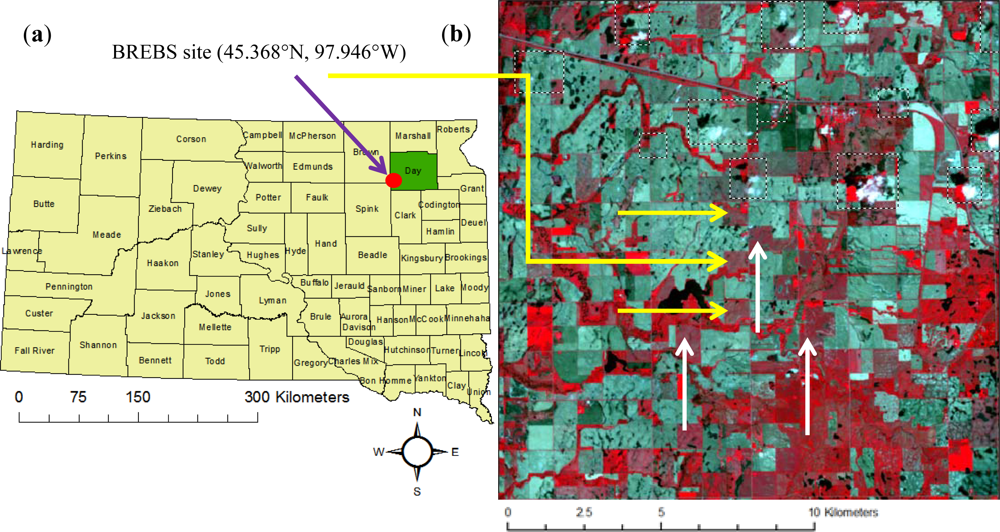
2.2.1. Location of Site

The BREBS is located on a cooperator’s field in western Day County, South Dakota; see Figure 1. The site was chosen for its expanse and relative levelness, and the specific field was chosen for the cooperating producer’s use of cover crops in the crop rotation. Within the field, the BREBS needed to be at least 200 m from any edge of the field so that the wind, temperature and humidity readings for the crop would not be affected by any surrounding features. A slight rise in the middle of the field was chosen for the BREBS site, so that minor flooding could be avoided. Data collection using the BREBS started on 25 May 2011 (DOY 145).

2.2.2. Crop Rotation

Spring wheat (Triticum aestivum L.) was planted on the field using a seed drill on 29 April 2011 (DOY 119). At the time of the BREBS installation, the crop height averaged 8 cm. The wheat was harvested 5 August 2011 (DOY 217). Within the area occupied by the BREBS, the wheat was cut using a motorized sickle and delivered to the cooperator’s harvester. A cover crop mixture of rye (Secale cereal L.), field radishes (Raphanus sativus L.) and field peas (Pisum sativum L.) was planted using a seed drill on 12 August 2011 (DOY 224). Within the BREBS area, the cover crop was planted using a single disc hand planter with a modified seed disc to accommodate multiple seeds per hole, with the same seed composition and planting rates as the rest of the field. Killing frost, signaling the end of the cover crop season, was the night of 18 October 2011 (DOY 291).

2.2.3. Calculation of EToF from BREBS Data

Grass-based reference evapotranspiration (ETo) is calculated using the ASCE Standardized Penman-Monteith equation [2]:
E T o = 408 Δ ( R n G ) + γ 37 T h r + 273 u 2 ( e ( T h r ) e a ) Δ + γ ( 1 + C d u 2 )
where:
ETo
= grass based reference evapotranspiration (mm · hr−1);
Rn
= net radiation at the grass surface (MJ m−2 · h−1);
G
= soil heat flux density (MJ m−2 · h−1);
Thr
= mean hourly air temperature (°C);
Δ
= saturation slope vapor pressure curve at Thr (kPa° · C−1);
γ
= psychrometric constant (kPa° · C−1)
(Thr)
= saturation vapor pressure at air temperature Thr (kPa);
ea
= average hourly actual vapor pressure (kPa);
Cd
= diurnal constant (0.24 s · m−1during daytime, 0.96 s · m−1during nighttime);
u2
= average hourly wind speed at 2 m (m · s−1).
The net radiation was calculated from solar radiation measured by the BREBS; Ta and ea were measured by the BREBS. Wind speed was measured at 3 m above the ground surface and adjusted to 2 m using the logarithmic wind profile equation as recommended by ASCE-EWRI [2]. After ETo is calculated on a per hour basis, daily values are calculated as the sum of the 24 hourly values. Also summed into daily values are the calculations of λE (latent heat flux) that the BREBS records. In a field setting, the only significant source of latent heat flux is water evaporation. Thus, the amount of latent heat used to evaporate water can be calculated using the Bowen ratio [19]. Evaporation based on the latent heat of vaporization (ETλE) is calculated by converting the latent heat portion of incoming energy to an equivalent depth of water (mm H2O) per day using the latent heat of vaporization of water and the appropriate length and mass unit conversions.
ETλE is an estimation of the actual evapotranspiration, and so the EToF can be calculated using the BREBS as:
E T o F = E T λ E E T o

2.3. Preparation of the Images

We used Landsat imagery path 30, row 28, for the analysis. Because the study area is located towards the center of the image, Landsat 7 imagery was used without losing much information caused by the SLC-off gaps. When selecting the images, we visually screened both Landsat 5 and Landsat 7 images and, based on our judgment, assigned each image a clearness fraction index between 0 and 1, with 0 being a completely cloudy and unusable image and 1 being a cloud-free image. The indices for each image date are shown in Table 1. Images with a clearness index greater than 0.8 were used in the METRIC model. The image from 8 September (DOY 251) was unusable due to incongruencies in the image registration relative to ground control points that occurred during the image pro-processing of the image at the USGS EROS Data Center.

2.3.1. Cloud Masking

The land surface in three of the images we used was partly obscured by clouds, requiring masking and interpolation from preceding and subsequent images. The three images containing cloud cover were from 11 May (DOY 131), 4 June (DOY 155) and 6 July (DOY 187). The clouds were manually identified and masked out. The resulting gaps were filled as described by Kjaersgaard and Allen [15] and Kjaersgaard et al.[20]. The method starts with the preceding image and looks at the image immediately following the image to be gap-filled to interpolate pixel values for the masked area. If the image immediately following the image to be gap-filled also has pixels that have been masked in the same location, then the model looks at the next image, and so on.

2.3.2. Spline Interpolation

Interpolation of the images in order to produce daily EToF maps was performed using a cubic spline function model [17]. This model has a built-in dampening function, which buffers the extreme ends of the EToF range. This buffer restrains EToF values from going much below zero or above 1.2.

2.3.3. Adjustment for Wet Image

Due to the extremely wet nature of the DOY 227 image, the tension of the spline interpolation was tightened to better restrict the high-end EToF values. Before this adjustment, the model incorrectly interpolated the EToF values from the DOY 187 image, the inflated EToF values from the DOY 227 image and the sharp drop in values from the DOY 235 image. Since the DOY 227 image and the DOY 235 image are only eight days apart, whereas there are 40 days between DOY 187 and DOY 227, the model analyzed the sharp drop in values and created a cubic spline that would fit such a drop. This resulted in artificially high EToF values that—before adjustment—were not effectively dampened.

2.3.4. Synthetic Images

The implementation of the cubic spline model creates daily maps one month at a time. To do this, it looks at two images before the month in question, one image taken during the month and two images after the month. For the first month of the season, May, the image from 3 May (DOY 123) was used in triplicate for both of the precedent images—29 and 30 April (DOY 119 and 120)—as well as for DOY 123. This was appropriate because of the close temporal proximity between DOY 123 and the precedent images, so change in vegetation—and transpiration—would be minimal. Also to consider would be soil evaporation, but based on data gathered from the Automatic Weather Data Network (South Dakota Department of Climate and Weather), soil conditions on DOY 123 were very similar to soil conditions on DOY 119 and 120, and no rain occurred during that period. For the last two images, DOY 275 and 291, synthetic images were created to estimate 1 and 2 November (DOY 305 and 306). Because DOY 305 and 306 were well after killing frost, we assumed bare soil devoid of vegetation (a common assumption for non-growing periods), and any ET would come from evaporation of residual soil moisture. Using meteorological information gathered from the BREBS, a daily soil water balance was used to estimate the soil evaporation reduction coefficients for DOY 305 and 306, which were found to be 0.06 and 0.05, respectively. With this information, two synthetic images, the first with a uniform value of 0.06 and the second with a uniform value of 0.05, were created to represent DOY 305 and 306 and inserted into the cubic spline model for the month of October.
Within the 260 km2 image area, there are two other fields that were under the same crop rotation (wheat followed by cover crop) as the field with the BREBS in it. One is located one mile to the north and the other is located one mile to the south, as shown in Figure 1(b). The fields are therefore denoted as the south field, the middle field (which contains the BREBS), and the north field. For comparison, three other fields where chosen that also were planted into wheat, but no cover crop was planted after harvest. These fields are denoted as the west field, the central field and the east field. Exact planting and harvesting dates for the fields without the BREBS are unknown, but personal observations of the area during the growing season indicate that the planting and harvesting dates were similar for all the fields.

2.4. Collation of the Data

Using Erdas Imagine, areas of interest were drawn around the edge of each of the three fields and buffered 60 m in from the edge, to avoid any “bleeding” caused by the coarser resolution of the thermal band. Daily EToF values were extracted for each pixel within the fields and brought into Microsoft Excel, such that each row represents an individual pixel from within the area of interest and each column represents a day. Hence, there are daily values for each pixel within the three fields from 1 May (DOY 121) to 1 November (DOY 305). The fields are uniquely shaped and, thus, do not have equal numbers of pixels. The middle field has 485 pixels, while the north field has 357 and the south field has 505. In total, 1,347 pixels were used to calculate an EToF curve (i.e., a crop coefficient curve) based on the METRIC data and its standard deviation found in Figure 2(a). For the non-cover cropped fields: the central field has 424 pixels, while the west field has 511 and the east field has 1,024. In total, 1,959 pixels were used to calculate the METRIC curve and its standard deviation found in Figure 2(b).

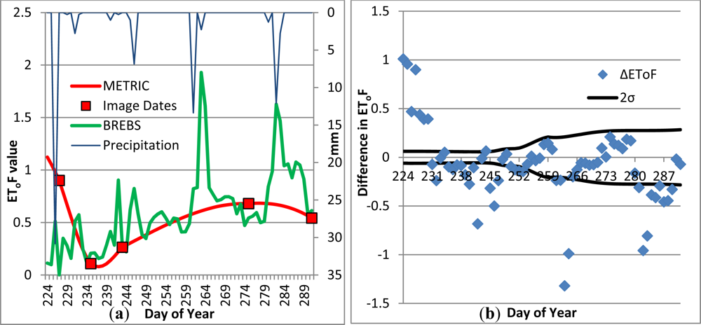
3. Results and Discussion

3.1. Analysis of the EToF Curves

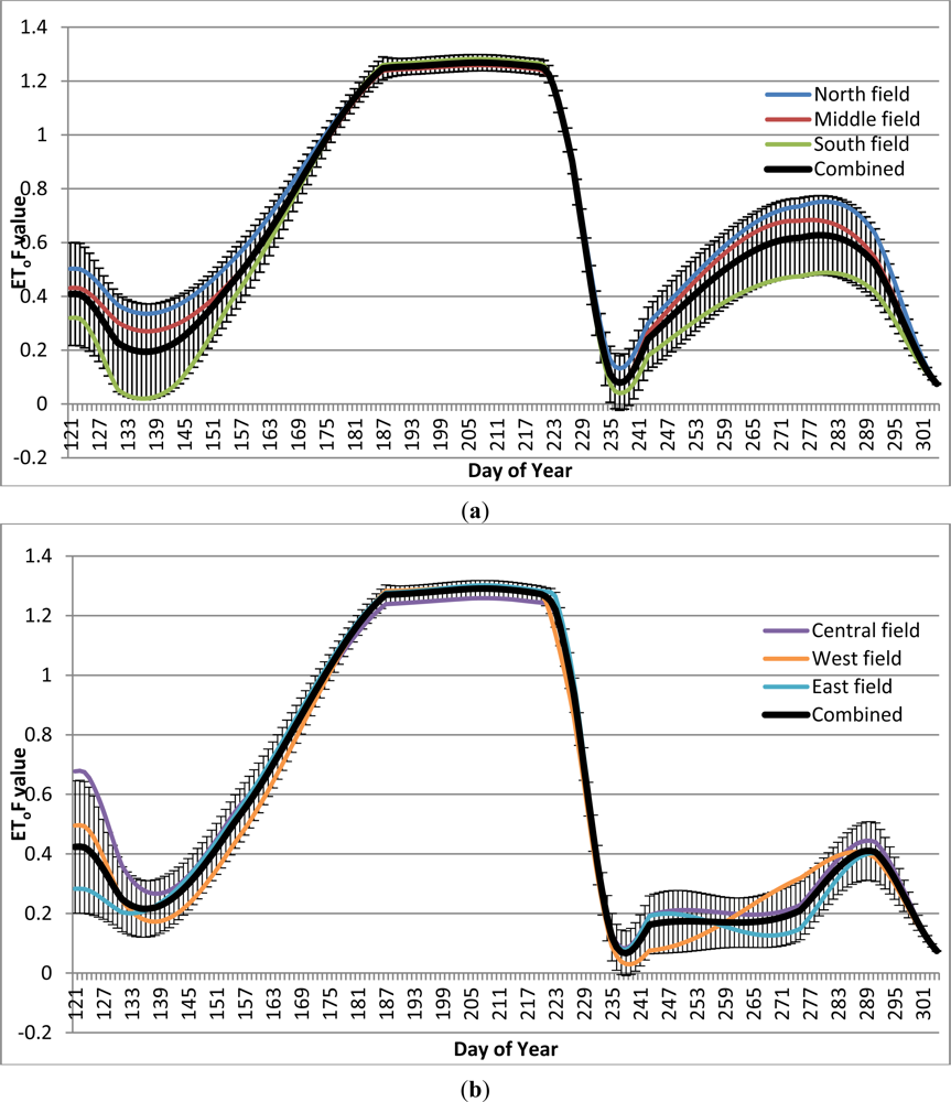
3.1.1. Fields with Cover Crops

In each of the three field sites, a distinct pattern arose when plotting the EToF pixel values for the May through October growing season. In early May, the fields were wet, which gave the pixels a high starting EToF value due to the high soil evaporation. This was also the time when the pixel values are the most spread out. One standard deviation from the combined mean was 0.19. As May progressed, the fields dried, and EToF dipped in the south field down to zero, ±0.2. In the middle field, EToF dipped down to 0.3 ± 0.2 and in the north field down to 0.4 ± 0.2. Towards the end of May was when the crop coefficient curve becomes readily distinguishable, as the pixel values began to group together and rise through the crop development stage until early July, when the curve flattens as the crop reached midseason values. In all the fields, the midseason EToF values are between 1.2 and 1.3. Noteworthy was the increase from the established FAO-56 spring wheat midseason crop coefficient value of 1.15 [1]. This departure is partly due to the fact that values calculated for the FAO-56 document are from research that is at least 15 years old. In that time, wheat varieties have improved and farming practices have evolved to produce higher yielding (and higher transpiring) crops. Another possible reason for the higher midseason EToF values was that the ground-based weather data for calculating ETo in METRIC was provided by the BREBS, which does not represent a grass-based reference surface. This could slightly deflate the ETo values and, thereby, inflate the EToF values. The crops remained in midseason until the middle of August, when the EToF values plunged over the course of 10 days, as the crop senesced to values ranging from just below zero to 0.5, with most values between zero and 0.2. Immediately after this plunge, the EToF values began to rise again, as the cover crop began to grow. In the middle field, the EToF curve reached its peak near DOY 275 with values ranging from 0.4 to 0.9, with most values between 0.6 and 0.8. In the north field, the EToF curve generally exceeded that of the middle field and had values that peaked between 0.7 and 0.8 around DOY 280. The south field also peaked around DOY 280, but its values were noticeably lower than in the other two fields, with values ranging between 0.3 and 0.8, most of which are between 0.3 and 0.6. Figure 2(a) shows the mean from each of the three fields, as well as the combined mean for all the fields.
It is clear that the values were the most variable at the beginning of the season and during the cover crop season. The variability at the beginning of the season could be due to uneven distribution of snowmelt and residue from the previous crop. Note from Figure 2(a) that from the second week of May (DOY 128) until June (DOY 152), half of the EToF values for the south field were more than one standard deviation less than the mean. The same was true of the south field from DOY 260-280, at the peak of the cover crop season. The three fields became very similar in EToF values during midseason of the wheat crop and followed each other closely through the steep decline in the middle of August. Outside of this time period, the EToF values of the south field were generally less than the average, whereas the middle and north field were generally higher than the average, with the north field having had slightly higher values than the middle field.

3.1.2. Fields without Cover Crops

The EToF curve for the wheat season shown in Figure 2(b) was very similar to the one in Figure 2(a). May opened with EToF values scattered around 0.4. It was at the very beginning of the season that the values were most spread out, with one standard deviation from the combine mean being 0.22. Looking at the means of each of the fields in Figure 2(b), the central field started the growing season with more than half of the pixel values at or higher than one standard deviation above the combined mean. The west field started out above the combined mean, and the east field below it, but they switched positions by the middle of May (DOY 134). All three fields dipped in the middle of May and then grouped together as they began the ascent for the development stage of the wheat crop. From the middle of May (DOY 134) through the middle of August (DOY 235), the METRIC curve was almost identical to the one in Figure 2(a). After the wheat harvest, the METRIC curve rebounded slightly and stayed around 0.2 until the end of September. In October, the curve increased up to a peak around 0.4 following a 12 mm rain event on DOY 282, before dropping at the end of the season. One standard deviation was around 0.09 throughout the month of September and the first half of October. Both the central field and the east field remained vegetation-free following wheat harvest. They had a small peak in EToF values in early September (DOY 245) and then a larger peak in mid-October (DOY 290). Little or no post-harvest weed control was done in the west field and a small amount of volunteer weeds appeared in the fall. As a result, the west field did not have a peak in early September but climbed steadily until it peaked in mid-October (DOY 288), and in early October the mean west field EToF values were more than one standard deviation above the combined mean.

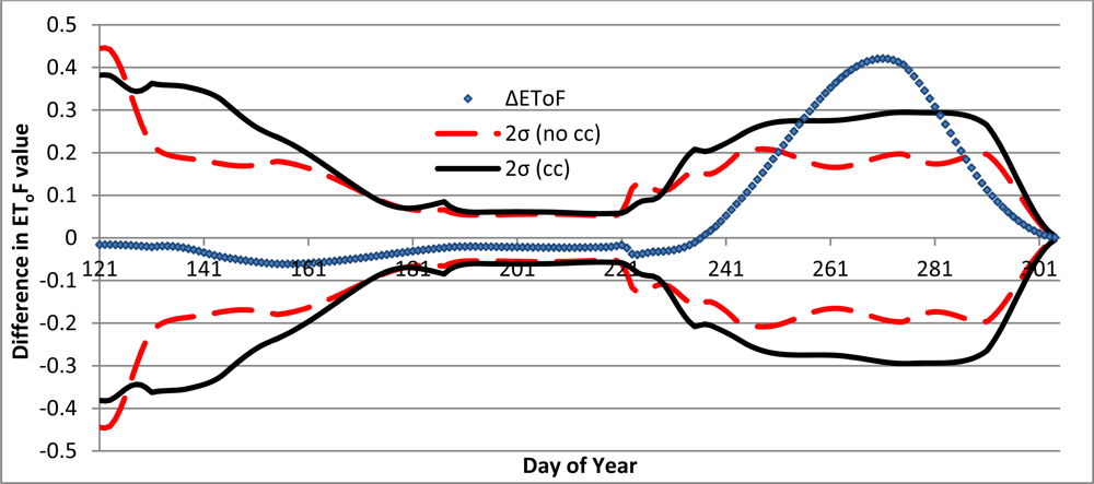
3.2. Cover Crop Season

There were five image dates during the cover crop season: DOY 227, 235, 243, 275 and 291. The wheat was harvested on 5 August (DOY 217), and the cover crop was planted on 12 August (DOY 224). From Figure 2(a), however, the METRIC-derived values do not show that week of fallow until DOY 235, which is August 23. This was because on the 14 August (DOY 226), there was a large rain event that resulted in very high EToF values for the 15 August (DOY 227) image. Because of this, the graph in Figure 2(a) does a very quick turnaround after DOY 235, when in actuality, the EToF values had been largely below 0.2 since DOY 217. Another cause for this discrepancy was the fact that the last image date during the wheat season was DOY 187, when the wheat was in midseason form. There were no useable images during the wheat crop’s senescence, and therefore, no reference for METRIC to begin a downslope. The METRIC curves shown in Figure 2(a,b) were very similar throughout the wheat season and only really began to differ after the wheat was harvested. Figure 2(a) shows that the cover crop raised the EToF values to a peak of around 0.7 in early October (DOY 279) with one standard deviation reaching maximum values of 0.15 at around the same time. Figure 2(b), on the other hand, shows no such increase in EToF values until a small rise in mid-October (DOY 289) that reached a peak of around 0.4 with one standard deviation of around 0.1. The difference in EToF between fields with and without cover crops is shown in Figure 3. From Figure 3, note that the difference between the two combined means stayed well within two standard deviations of either combined mean until the cover crop season. Even with the relatively large standard deviation of the combined mean in Figure 2(a) from DOY 250 to DOY 290, the difference between the two curves was well outside of two standard deviations from the combined means. This indicated a distinct difference in estimated ETa rates for the period from the middle of September to the middle of October.

Statistical Analysis

Though both the METRIC model and calculations from the BREBS attempt to close the energy balance equation, their methods of doing so are very different and should be viewed as such. That being said, Figure 4(a,b) shows the results from each graphed together and the difference between them. With the BREBS, precipitation events promptly result in spikes in the EToF values. With METRIC, there were only five image dates to provide data. Since the daily data points were interpolated between image dates, and daily precipitation amounts are not included in METRIC, the EToF graph is a relatively smooth curve. As Figure 4(a) shows, after a rain event, the BREBS curve spiked, but after a few days returned to approximately the value of the METRIC curve. DOY 217 (5 August) was the harvest date and represented essentially bare soil conditions. However, METRIC was unable to follow the ground-based data here because of the wet conditions of the DOY 227 image; such high rates of estimated ETa (even though it was all soil evaporation) indicated a healthy, growing field.
The absence of a sharp spike in the BREBS values after the rain event on DOY 226 was because the BREBS was struck by lightning and data entries were damaged, so 30 hours needed to be removed from the record. The next image after DOY 227 was DOY 235, and as Figure 4(a) shows, METRIC had detected the drop in EToF values. After DOY 235, METRIC showed a crop coefficient curve that generally followed the BREBS curve. The METRIC curve approached 0.7 at the beginning of October (DOY 279) before falling off at the end of the season; there was no sudden drop like at the end of the wheat season because there was no harvest of the cover crop, only decreasing temperatures and shortening days. There also did not seem to be much of a midseason, such as there was during the wheat crop. This is due to the slow growth of the cover crop caused by its late season planting, as well as lack of rainfall.
Figure 4(b) shows the difference between the daily EToF values calculated by METRIC and by the BREBS. Note that the BREBS curve was based on daily data, whereas the METRIC curve was based on five snapshots taken over the course of three months. Therefore, the BREBS curve acts more like a dual crop coefficient curve, with a basal crop coefficient curve and spikes indicating the soil evaporative component. On the other hand, the METRIC curve acts like a single crop coefficient curve, interpolating many days between image dates and creating a smooth crop coefficient curve. Thus, Figure 4(b) should be analyzed qualitatively. In all, 30 of the 68 days that made up the cover crop season (DOY 224–291) were within two standard deviations of the METRIC values. The first 10 days were residuals from the METRIC curve pre-August 15 (DOY 227), however, and after that, 29 of the 58 remaining days were within two standard deviations of the METRIC values. Considering that METRIC aggregates EToF values between precipitation events, to have 50% of the BREBS values within two standard deviations of the METRIC curve is noteworthy. More telling is the fact that, after 23 August (DOY 235), only once was the METRIC value more than two standard deviations higher than the BREBS value. This shows that, while the BREBS values may spike, when they return to values primarily driven by transpiration, their values and METRIC’s were reasonably close. By removing the day of and the day after precipitation events, the number of BREBS values within two standard deviations of the METRIC curve jumped to 27 of 42 days (64%).
The sum depth of estimated ETa shown in Table 2 shows that the METRIC estimates are very similar to the BREBS estimates for the cover crop season, with only a 7% difference between the sums. That the sum of the METRIC values wasn’t much lower than the sum of the BREBS values (judging by Figure 4(a) this should be the case) was due to fact that when the BREBS measured a high EToF, it invariably coincided with a precipitation event. On precipitation days, ETo is very low, thus measured ETλE can be a large fraction of ETo without having a very large value. The cumulative estimated ETa from the fields without a cover crop during the period from 12 August (DOY 224) to 18 October (DOY 291) was 59% of the cumulative estimated ETa from the fields with a cover crop.

4. Conclusions

The cover crop mixture of rye/radish/pea was never able to fully develop due to several factors: declining temperatures slowed maturation, shortening days reduced available energy, and inadequate precipitation limited growth. Additionally, the cover crop was planted more sparsely than a typical cash crop and, thus, barring much increased individual plant growth, would not be able to generate the ETa (actual evapotranspiration) of a healthy, densely planted cash crop, such as wheat. Clearly, the cover crops did not reach, let alone maintain, the estimated ETa rates of the previous wheat crops—with cover crop EToF rates peaking around 0.6, while wheat maintained around 1.25 for a month—but they did generate more than enough ETa for METRIC (Mapping Evapotranspiration at high Resolution with Internalized Calibration) to detect and create an EToF (fraction of reference evapotranspiration) curve. METRIC estimated that the ETa of fields with cover crops planted after wheat was 52 mm more than the fields without covers crops planted (from the date of cover crop planting until the first killing frost). Admitting some time lag in the METRIC EToF curve following the wheat harvest, METRIC did well in comparison with BREBS (Bowen-Ratio Energy Balance System)-derived EToF, though it was more useful as a single crop coefficient, whereas the BREBS EToF acted like a dual crop coefficient. Total estimated ETa from the BREBS and METRIC for the cover crop season compared well, with the BREBS estimating 136 mm of ETa and METRIC estimating 127 mm of ETa, only a 7% difference between the sums. In conclusion, METRIC did well in estimating ETa for a non-traditional crop that was both late season and short season. Despite the relative dearth of available data points, METRIC detected the increased vegetative activity in the fields—which was by no means as vigorous as a cash crop—and successfully estimated an EToF curve.
The differences in the estimated ETa signal between fields that otherwise appeared to be managed under the same cropping system is not uncommon. As a result, in situ monitoring of ETa may not be entirely representative for a population of fields. We found that the use of remote sensing to estimate the spatial distribution of ETa was encouraging. Using remote sensing-based estimates of ETa can help document differences in water use between fields across a region, thereby providing critical information for water resources management.

List of Principal Acronyms and Abbreviations

BREBS
Bowen-Ratio Energy Balance System;
ET
Evapotranspiration (mm);
ETa
Actual evapotranspiration (mm);
ETcc
Estimated actual evapotranspiration of fields planted into cover crop after wheat (mm);
ETno cc
Estimated actual evapotranspiration of fields not planted into cover crop after wheat (mm);
ETo
Grass-based reference evapotranspiration (mm);
EToF
Fraction of grass-based reference crop evapotranspiration (unit-less);
ETλE
Estimated actual evapotranspiration using BREBS data (mm);
Kc
Ideal crop coefficient (unit-less);
METRIC
Mapping Evapotranspiration at high Resolution using Internalized Calibration.

Acknowledgments

We would like to thank Roger and Grant Rix for their cooperation in providing the field site for the BREBS. We thank Todd Trooien, Laura Edwards, Nathan Brandenburg, Eric Stearns, Christian Karels, Patrick Hofer, Grzegorz Brudecki, Iwona Cybulska, Doug Hankerson and Cheryl Reese for their assistance during the project. Funding for the BREBS is provided by the National Institute of Food and Agriculture, USDA, under Agreement No. 2008-51130-19548. Additional funding is provided by the South Dakota Experiment Station and the South Dakota Water Resources Institute.

References

  1. Allen, R.G.; Pereira, L.S.; Raes, D.; Smith, M. Crop Evapotranspiration. Guidelines for Computing Crop Water Requirements. In FAO Irrigation and Drainage Paper 56; FAO: Rome, Italy, 1998; p. 300. [Google Scholar]
  2. ASCE-EWRI. The ASCE Standardized Reference Evapotranspiration Equation. In ASCE-EWRI Standardization of Reference Evapotranspiration Task Committee Report; ASCE: Reston, VA, USA, 2005; p. 216. [Google Scholar]
  3. Allen, R.G.; Tasumi, M.; Trezza, R. Satellite-based energy balance for Mapping Evapotranspiration with Internalized Calibration (METRIC)—Model. J. Irrig. Drain. Eng 2007, 133, 380–394. [Google Scholar]
  4. Dabney, S.M.; Delgado, J.A.; Reeves, D.W. Using winter cover crops to improve soil and water quality. Commun. Soil Sci. Plant Anal 2001, 32, 1221–1250. [Google Scholar]
  5. Keim, B.D. The lasting scientific impact of the Thornthwaite water-balance model. Geol. Rev 2010, 100, 295–300. [Google Scholar]
  6. Allen, R.G.; Irmak, A.; Trezza, R.; Hendrickx, J.M.H.; Bastiaansseen, W.; Kjaersgaard, J. Satellite-based ET estimation in agriculture using SEBAL and METRIC. Hydrol. Process 2011, 25, 4011–4027. [Google Scholar]
  7. Prueger, J.H.; Hatfield, J.L.; Sauer, T.J. Surface energy partitioning over rye and oats cover crops in central Iowa. J. Soil Water Cons 1998, 53, 263–268. [Google Scholar]
  8. Hay, C.H.; Irmak, S. Actual and reference evaporative losses and surface coefficients of a maize field during nongrowing (dormant) periods. J. Irrig. Drain. Eng 2009, 135, 313–322. [Google Scholar]
  9. Ruhoff, A.; Paz, A.; Collischonn, W.; Aragao, L.; Rocha, H.; Malhi, Y. A MODIS-based energy balance to estimate evapotranspiration for clear-sky bays in Brazilian tropical savannas. Remote Sens 2012, 4, 703–725. [Google Scholar]
  10. Teixeira, A. Determining regional actual evapotranspiration of irrigated crops and natural vegetation in the São Francisco River Basin (Brazil)—Using remote sensing and Penman-Monteith equation. Remote Sens 2010, 2, 1287–1319. [Google Scholar]
  11. Chavéz, J.; Gowda, P.; Howell, T.; Garcia, L.; Copeland, K.; Neale, C. ET mapping with high-resolution airborne remote sensing data in an advective semiarid environment. J. Irrig. Eng 2012, 138, 416–423. [Google Scholar]
  12. Bastiaanssen, W.G.M.; Menenti, M.; Feddes, R.A.; Holtslag, A.M.M. A remote sensing Surface Energy Balance Algorithm for Land (SEBAL): 1. Formulation. J. Hydrol. 1998, 212–213, 198–212. [Google Scholar]
  13. Tasumi, M.; Trezza, R.; Allen, R.G.; Wright, J.L. Operational aspects of satellite-based energy balance models for irrigated crops in the semi-arid US. J. Irrig. Drain. Eng 2005, 19, 355–376. [Google Scholar]
  14. Allen, R.G.; Tasumi, M.; Morse, A.T.; Trezza, R.; Kramber, W.; Lorite, I.; Robison, C.W. Satellite-based energy balance for Mapping Evapotranspiration with Internalized Calibration (METRIC)—Applications. J. Irrig. Drain. Eng 2007, 133, 395–406. [Google Scholar]
  15. Kjaersgaard, J.; Allen, R.G. Remote Sensing Technology to Produce Consumptive Water Use Maps for the Nebraska Panhandle; Kimberly R&E Center-University of Idaho: Aberdeen, ID, USA, 2010; p. 88. [Google Scholar]
  16. Irmak, A.; Ratcliffe, I.; Ranade, P.; Hubbard, K.; Singh, R.K.; Kamble, B.; Kjaersgaard, J. Estimation of land surface evapotranspiration with a satellite remote sensing procedure. Great Plains Res 2011, 21, 73–88. [Google Scholar]
  17. Kjaersgaard, J.; Allen, R.G.; Irmak, A. Monthly and growing season ET estimation from moderate-resolution satellites with accounting for precipitation events. Hydrol. Process 2011, 25, 4028–4036. [Google Scholar]
  18. Bastiaanssen, W.G.M. Regionalization of Surface Flux Densities and Moisture Indicators in Composite Terrain: A Remote Sensing Approach under Clear Skies in Mediterranean Climates. CIP Data Koninklijke Bibliotheek, Den Haag, The Netherlands, 1995; p. 273. [Google Scholar]
  19. Bowen, I.S. The ratio of heat losses by conduction and by evaporation from any water surface. Phys. Rev. C Nucl. Phys 1926, 27, 779–787. [Google Scholar]
  20. Kjaersgaard, J.; Trezza, R.; Allen, R.; Robison, C.; Oliveira, A.; Dhungel, R.; Kra, E. Filling Satellite Image Cloud Gaps to Create Complete Images of Evapotranspiration. Proceedings of Remote Sensing and Hydrology 2010 Symposium, Jackson Hole, WY, USA, 27–30 September 2010.
Figure 1. (a) Location of the study site within South Dakota with county boundaries indicated. The arrow points to the study area. BREBS site is located at 45.368°N, 97.946°W. (b) The false color image of the study area from 4 June 2011, dotted-line boxes show the areas to be masked for gap-filling. The three yellow arrows indicate the three fields that were planted into cover crop after spring wheat, with the BREBS located in the middle field. The three white arrows indicate three fields that were not planted into cover crop after spring wheat.
Remotesensing 04 03796f1
Figure 2. (a) Daily average EToF (unit-less) values calculated with METRIC for three fields that used a cover crop mixture of rye/radish/pea after a cash crop of wheat. Included is a combined average with error bars showing one standard deviation of the 1,347 sampled pixels. (b) Daily average EToF values calculated with METRIC for three fields that did not use a cover crop after a cash crop of wheat. Included is the combined average, with error bars showing one standard deviation of the 1,959 sampled pixels.
Remotesensing 04 03796f2
Figure 3. Difference between METRIC EToF values (unit-less) calculated for the fields with cover crops and for the fields without cover crops. The blue points are the difference in EToF values between fields with cover crops and fields without cover crops. The black lines represent two standard deviations from the combined mean of the fields with cover crops, and the red dashed lines represent two standard deviations from the combined mean of the fields without cover crops.
Remotesensing 04 03796f3
Figure 4. (a) EToF values (unit-less) for the cover crop season calculated from the BREBS and from METRIC. Precipitation is also shown. Image dates were DOY 227, 235, 243, 275 and 291. (b) Difference between METRIC values and BREBS values, the lines represent ±2 standard deviations from the mean of the METRIC EToF estimates.
Remotesensing 04 03796f4
Table 1. Image dates (year 2011) with clearness index and Landsat satellite from which the image was taken. Bolded entries indicate images that have an index greater than 0.8 and that were used in METRIC.
DoyLs #Clearness IndexDoyLs #Clearness IndexDOYLS #Clearness Index
1237118770.9251*70.95
13150.951955025950
13970.420370.726770.8
1475021150.527551
15570.8521970.5528370
163502275129151
171702357129970.2
17950.7524351
*The image from DOY 251 was removed due to incongruencies in its spatial coordinates.
Table 2. Sum of ETo, ETa estimated from the BREBS (ETλE), ETa estimated from METRIC for the cover cropped fields (ETcc), and non-cover cropped fields (ETno cc), and precipitation for the cover crop season (12 August through 18 October (DOY 224–291) 2011).
MeasurementDepth (mm)
ETo (BREBS)266
ETλE (BREBS)136
ETcc (METRIC)127
ETno cc (METRIC)75
Precipitation75

