Estimating Crop Coefficients Using Remote Sensing-Based Vegetation Index

1
Department of Civil Engineering, 3310 Holdrege Street, University of Nebraska-Lincoln, Lincoln, NE 68583, USA
2
School of Natural Resources, 3310 Holdrege Street, University of Nebraska-Lincoln, Lincoln, NE 68583, USA
*
Author to whom correspondence should be addressed.
Remote Sens. 2013, 5(4), 1588-1602; https://doi.org/10.3390/rs5041588
Submission received: 11 January 2013
/
Revised: 13 March 2013
/
Accepted: 15 March 2013
/
Published: 26 March 2013
(This article belongs to the Special Issue Advances in Remote Sensing of Crop Water Use Estimation)
Abstract
:Crop coefficient (Kc)-based estimation of crop evapotranspiration is one of the most commonly used methods for irrigation water management. However, uncertainties of the generalized dual crop coefficient (Kc) method of the Food and Agricultural Organization of the United Nations Irrigation and Drainage Paper No. 56 can contribute to crop evapotranspiration estimates that are substantially different from actual crop evapotranspiration. Similarities between the crop coefficient curve and a satellite-derived vegetation index showed potential for modeling a crop coefficient as a function of the vegetation index. Therefore, the possibility of directly estimating the crop coefficient from satellite reflectance of a crop was investigated. The Kc data used in developing the relationship with NDVI were derived from back-calculations of the FAO-56 dual crop coefficients procedure using field data obtained during 2007 from representative US cropping systems in the High Plains from AmeriFlux sites. A simple linear regression model (KcNDVI = 1.457 NDVI – 0.1725) is developed to establish a general relationship between a normalized difference vegetation index (NDVI) from a moderate resolution satellite data (MODIS) and the crop coefficient (Kc) calculated from the flux data measured for different crops and cropping practices using AmeriFlux towers. There was a strong linear correlation between the NDVI-estimated Kc and the measured Kc with an r2 of 0.91 and 0.90, while the root-mean-square error (RMSE) for Kc in 2006 and 2007 were 0.16 and 0.19, respectively. The procedure for quantifying crop coefficients from NDVI data presented in this paper should be useful in other regions of the globe to understand regional irrigation water consumption.
1. Introduction
The crop coefficient (Kc)-based estimation of crop evapotranspiration (ETc) is one of the most commonly used methods for irrigation water management at the field scale. Crop evapotranspiration (ETc) can be calculated using the Kc defined as the ratio of crop evapotranspiration to some reference evapotranspiration (ETo) defined by weather data [1,2]. In this framework, Kc values are specific to each crop (and to the method used for ETo) and have traditionally been derived from data sets, where measured ETc for a well-watered crop is divided by a standard reference ETo (usually grass, but sometimes alfalfa and, most recently, not crop-specific, but only a tall or short crop [3])). The crop coefficients representative of well watered conditions are tabulated for the practical purpose of crop water management among engineers, farmers and irrigation managers [3–5]. During the crop growing season, the value of Kc for most agricultural crops increases from a minimum value at emergence, in relation to changes in canopy development, until a maximum Kc is reached at about full canopy cover. A crop coefficient curve is the seasonal distribution of Kc, often expressed as a smooth continuous function in time or some other time-related index. The Kc tends to decline at a point after a full cover is reached in the crop season. The declination extent primarily depends on the particular crop growth characteristics [6,7] and the irrigation management during the late season [1]. Crop coefficients primarily depend on the dynamics of canopies, light absorption by the canopy, canopy roughness, which affects turbulence, crop physiology, leaf age and surface wetness [4]. As a crop canopy develops, the ratio of transpiration to evapotranspiration increases, until most of the evapotranspiration comes from transpiration, and soil evaporation is a minor component. This occurs because the interception of radiant energy by the foliage increases until most light is intercepted before it reaches the soil. Moreover, the relationships between spectral indices and crop coefficients are usually observed for the single crop coefficient. The normalized difference vegetation index (NDVI) has been used extensively for vegetation monitoring, crop yield assessment and drought detection [4,6–8]. Higher NDVI indicates a greater level of photosynthetic activity [8,9]. Increase in crop coefficient caused by higher temperature results in a decrease in soil water and a decline of NDVI, while dense vegetation induces more evapotranspiration and lowers the land surface temperature [10]; or the transpiring canopy is cooler [11]. On the regional scale, the current procedure to estimate Kc and resulting consumptive water use has limitations. The Kc varies in space and in time, due to inherent variability in emergence date, land use pattern, antecedent precipitation, emissivity, vegetation amount and atmospheric boundary conditions, such as air temperature, wind speed and vapor pressure deficit.
A number of researchers have used multispectral vegetation indices derived from remote sensing to estimate Kc values at the field scale for maize [11–15], wheat, cotton [11] and beans [13,14]. Bausch and Neale demonstrated application of ground based physical remote sensing technique to relate seasonal NDVI to Kc[15–17]. Several researchers [8,15–22] have shown that vegetation indices from remote sensing could be used to predict “basal” crop coefficients for agricultural crops. Bastiaanssen has discussed in detail the need to develop a methodology to determine aerial crop coefficient values for different agriculture land use patterns and practices [12]. Relationships between crop growth parameters, meteorological variations and tillage practices encourage researchers to study the experimental retrieval of crop coefficients at the field or regional scale. Leaf area index (LAI) has been estimated by several researchers using NDVI [23,24], even though the crops they were monitoring were both stressed and unstressed and, sometimes, were different crops. In the same manner we are looking at rainfed and irrigated crops to determine if NDVI explains the variations between the crop coefficients. Techniques are needed to map Kc weekly or biweekly for the purpose of consumptive water use calculation at the field or regional scale. With the launch of NASA’s MODerate resolution Imaging Spectroradiometer (MODIS) satellite, a new data set is available for utilization in daily crop monitoring for water management. The Terra-MODIS satellite provides eight-day composite images with a combination of spectral and thermal bands. The eight-day composite images are treated as cloud-free products to monitor the Earth’s terrestrial activity [7,20].
The objective of this study was to investigate the applicability of time-series MODIS 250 m normalized difference vegetation index (NDVI) data to the development of spatially representative Kc. We will discuss below a simple regression approach for the retrieval of Kc and provide a brief rationale for various components of the procedure. The specific objectives of this study were to (a) analyze the seasonal dynamics of crop coefficients (Kc) and the vegetation index (NDVI), (b) develop a regression model to establish the relationship between the NDVI and Kc values for agricultural production systems and (c) evaluate the performance of the new model for estimating Kc using an independent dataset for South-Central Nebraska. Implicit in our investigation is the assumption that NDVI is specific to the crop located at each pixel.
2. Material and Methodology
2.1. Study Area and Crop Evapotranspiration Dataset
This study is conducted using data from three different locations for climate conditions in the High Plains of the USA, located in the Midwest, between dense eastern forest and the western mountains and deserts. This area is focused on agriculture production and is composed of ranches and farms, where irrigated and rainfed farming systems present [25]. As of the last census of agriculture in 2007, there were 2.2 million farms, covering an area of 373.12 million ha. Major crops grown in this area are maize, sorghum, alfalfa, soybean, wheat and cotton. The first dataset is from agricultural production fields and part of an ongoing carbon sequestration research program at the University of Nebraska-Lincoln, Agricultural Research and Development Center (ARDC) near Mead, NE (Mead irrigated (center-pivot) continuous maize production system (48.7 ha), Mead irrigated (center-pivot) maize–soybean rotation (52.4 ha) and Mead rainfed maize–soybean rotation (65.4 ha)). All Mead sites are within 1.6 km of each other and are found on silty clay loam soils. We obtained the Level 4 data product for AmeriFlux sites over the period of 2007 from the AmeriFlux website ( http://public.ornl.gov/ameriflux) (Table 1). The second dataset is from a rainfed grassland site at Cottonwood, South Dakota. Both the Mead and Cottonwood sites are part of the AmeriFlux network [26], with detailed measurement activities. The third site is an irrigated agricultural field at the South Central Agricultural Laboratory (SCAL) (16 ha) located near Clay Center, NE, USA [26,27]. Mean annual precipitation of Mead is 704 mm, and annual precipitation for 2007 is 927 mm; while precipitation during the growing season (290–350 mm) received at the three sites during the growing seasons of 2006 and 2007 (Table 1; Figures 1 and 2) was significantly large, the rainfed fields were not stressed much and, therefore, were considered similar to the irrigated fields.
The field at South Central Agricultural Laboratory (SCAL) is an irrigated maize-soybean rotation with a center-pivot irrigation system. Table 1 shows the details of each field. We obtained the hourly temperature, latent heat flux data at 4 AmeriFlux [25,27] sites for the growing season of 2007 from the data repository at Oak Ridge National Laboratory (Figure 1; Table 1).
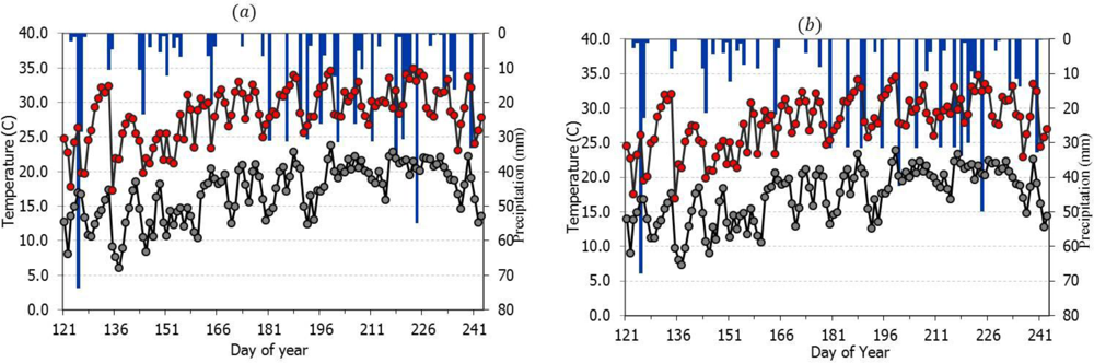
Figures 1 and 2 show the daily maximum (red) and minimum (gray) temperature and precipitation (blue) data at model calibration and model validation sites, respectively. These sites are distributed across the High Plains of the US and cover a wide range of agriculture vegetation types (Table 1). We also used a published dataset of crop coefficients from SCAL [28], obtained from NEBFLUX (Nebraska Water and Energy FLux Measurement, Modeling and Research Network) [13]. Both networks have micro-metrological towers that are used to monitor fluxes over agriculture sites.
2.2. NDVI and Kc Model Development and Validation
The Hargreaves and Samani (1985) equation is a temperature-based empirical method developed at Davis, California, using lysimeter data [29,30]. The Hargreaves and Samani (1985) equation is originally developed for time periods of five days or longer to reduce the influence of the temperature range, large variations in wind speed or cloud cover. Nevertheless, several studies have shown that the Hargreaves equation provides reliable estimates of daily ETo [14,30]. Daily reference crop evapotranspiration values were computed based on the equations presented by Hargreaves and Samani:
where ET0 is grass-reference evapotranspiration (mmd−1), Tmax is daily maximum air temperature (°C), Tmin is daily minimum air temperature (°C), Tmean is daily mean air temperature (°C) and Ra is extraterrestrial radiation (MJ·m−2·d−1).
KT is an empirical coefficient, which is a function of the temperature difference
Ra was calculated for each day using the equation and methodology of Duffie and Beckman [31]. ET0 for the four sites was estimated using the above equation throughout the growing season of 2007.
The MODIS instrument offers new possibilities for large-area crop mapping by providing a daily global coverage of high-quality, intermediate resolution (250 m) data since February 2000 at no cost to the end user. In an analysis of a MODIS surface reflectance 8-day composite, 250 m (MOD09) images were downloaded from the National Aeronautic and Space Administration (NASA) Land Process Distributed Active Archive Center (LPDAAC) ( https://lpdaac.usgs.gov/lpdaac/get data/data pool) for the study area. The normalized difference vegetation index (NDVI) [32] was derived from downloaded remote sensing data using near-infrared and red bands. The normalized difference vegetation index (NDVI) utilizes reflectance of the canopy in the near-infrared (NIR) and red (R) bands of the spectrum [32]. This vegetation index is given by:
where NIR is the reflectance in near infrared and R is the reflectance in the red region of the spectrum. The NDVI values are reported to be well correlated with vegetation parameters, like leaf area index, net primary productivity and gross primary productivity [23,33].
Crop coefficient (Kc) is used to calculate evapotranspiration. The ETc/ETo ratio is commonly referred to as the crop coefficient [1]. To develop an NDVI-Kc relationship requires ground-truth data for measured Kc values. We have used AmeriFlux data for modeling the NDVI-Kc relationship (Table 1), and Kc values from SCAL for 2006 and 2007 were used for validation purposes [28]. The daily Kc values from five locations (Table 1) for May, June, July and August were sampled for particular Day of Year (DOY) when NDVI values were available. To avoid mixed pixel problems, we used NDVI pixels located as close as possible to the center of the field. NDVI and satellite pass day for respective station geolocations (see Table 1) in 2006 and 2007 were extracted from the analyzed remote sensing dataset using ENVI software. For each satellite overpass date, we created a site and land use-specific dataset. The NDVI-Kc linear regression model can be used to identify the relationship between a single predictor variable NDVI and the response variable Kc when all the other predictor variables in the model are “held fixed”. The goal of regression analysis is to express the response variable as a function of the predictor variables. We used simple linear regression analysis to develop a relationship between NDVI and Kc, which can be applied to a satellite image:
where, for the ith case, KciNDVI is the response variable, NDVIi,1, NDVIi,2, ..., NDVIi,n are n repressors and εi is a mean zero error term. The quantities β0 and βj are unknown coefficients, whose values are determined by least squares regression, where β0 is the intercept and βj is slope for the jth term in the regression. The coefficients in the above equation were determined by the use of four different agriculture landuse datasets and DOY throughout the season, so that the above equation is applicable to a wide range of agriculture land use throughout the growing season. The coefficient of determination (r2) represents the proportion of variability in Kci that may be attributed to the linear combination of the independent variables. The coefficient of determination is used to assess the degree of fit (r2 = 0, no fit; r2 = 1, perfect fit) for the linear model shown in Equation (4):
To develop the above NDVI-Kc relationship, we did not conduct any site visits. Rather, we quantified the Kc, NDVI, their interactions and the actual evapotranspiration values for the natural conditions of the fields, as reflected in the MODIS satellite images [7,20]. The NDVI-Kc model was evaluated using data for another full season maize grown in the years 2006 and 2007 at the Clay Center (Table 1). We used regression analysis and root-mean-square error to evaluate the model. Regression analysis gives information on the relationship between the observed Kc variable and the predicted Kc variable to the extent that information is contained in the data. For validation, we used a plot of the observed Kc against the predicted Kc (using Equation (4)). Correlation between the actual and predicted Kc values was then calculated to assess the goodness of fit. The coefficient of determination (r2), which was used as a relative index of model performance, and root-mean-square error (RMSE) (reference) was used to compare the observed Kc and predicted Kc crop coefficients. This gave an indication of both bias and variance from the 1:1 line. The RMSE provides a good measure of how closely two independent data sets match.
3. Result and Discussion
3.1. Seasonal NDVI and Crop Coefficient Patterns for Selected Agricultural Land Use
We used the Ameriflux Mead sites and the Cottonwood site in 2007 as the model development dataset, while model validation datasets included the South-Central Agriculture laboratory of UNL in 2006 and 2007. The results of the temporal progression of NDVI and crop coefficients for the four selected sites for validation and modeling show that the phenology of the crops can be tracked by MODIS-based NDVI (Table 1). Figures 3 and 4 shows the NDVI patterns of the different agriculture land uses selected for modeling and validation. Irrigated maize from SCAL (Figure 4) shows smooth, increasing greenness intensity with the tendency to go down at the end of the season.
An increase in vegetation activity is also observed before the cropping season, because of the growth of vegetation at the onset of the spring rainy season. The respective fluctuation of crop coefficients for agriculture and grass is seen throughout the season, which shows the strong correlation between the NDVI and crop coefficients. The maximum NDVI of irrigated rotation, irrigated and rainfed maize peaks at 0.84 by the end of July (DOY 215) and 0.77 (DOY 221), respectively. It is obvious that the NDVI of irrigated maize is greater than that of rainfed maize throughout the growing season (Figure 4). Maize is usually planted in late April to early May and harvested in late September to early November.
It is interesting to note that the standard deviation for NDVI, as well as for Kc, of irrigated maize and irrigated rotation are almost the same while for rainfed NDVI and Kc are lower at the Clay Center for 2006 and slightly higher in 2007, but the crop coefficient standard deviation is almost the same (Table 2). During the growing season, the crop coefficient (Kc) for irrigated maize was approximately 0.3 ± 0.5 early in the season and 1.00 ± 0.05 during mid-season. From Mead Irrigated (a) and (b) conditions (Figure 4), when NDVI is high and the vegetation is unstressed, the crop coefficient is on average 1 and can reach 1.2, which shows that actual ET can be larger than the reference ET, which is defined for well-irrigated condition. While the condition in Mead Rainfed, Cottonwood and SCAL (Figure 3) shows that lower NDVI are associated with the rainfed condition, owing to the under-developed canopies and the lower capacity to absorb photosynthetically active radiation. Because of such a condition, the crop coefficient is below 1.1, which shows that actual ET can be less than the reference ET.
3.2. Development of NDVI and Crop Coefficient Relationship
In the development of the NDVI-Kc model to estimate the crop coefficient from remote sensing NDVI, we simplify an agriculture landscape as a mixture of only irrigated agriculture, rainfed agriculture and grass land. The ground measurement dataset of crop coefficients was collected from Ameriflux for the growing season of 2007 and SCAL for the growing season of 2006 [28]. We used the Mead sites and Cottonwood site in 2007 as the model development dataset, while model validation datasets were used from SCAL in 2006 and 2007. The statistics (maximum, minimum, mean and CV) for NDVI and crop coefficient values were given for each year for each site (Table 2). With the NDVI from remote sensing and the corresponding crop coefficient from field measurement, a simple linear regression equation was developed.
Figure 5 shows the relationship between NDVI and the crop coefficient for irrigated agriculture, rainfed agriculture and the combined relationship for irrigated and rainfed crops. There was a strong correlation between NDVI and the crop coefficient for all of the crops represented in the figure. The combined relationship between NDVI and the crop coefficient for rainfed and irrigated agriculture from all modeling locations is:
where 1.4571 and 0.1725 represent the slope and intercept coefficients. The correlation coefficient (r2) is 0.8259, which is highly informative about the amount of variance that NDVI can explain in the Kc data set, regardless of whether their joint distribution is normal. There was a strong correlation between NDVI and the crop coefficient for all of the crops represented in the Figure 5. The NDVI-Kc relationship for irrigated agriculture and rainfed agriculture is identical. There is no significant difference in the regression, slope and intercept coefficients for irrigated and rainfed agriculture data. Maize, both irrigated and rainfed, indicates a stronger relationship than for soybean. Furthermore, variation in NDVI and KcNDVI was larger during mid- and late season in rainfed maize fields than for irrigated. This could be attributed to variation in ETo, which increases evapotranspiration rates during crop development and senescence, and also, the frequent irrigation condition in irrigated field makes fields more evaporative, as compared to the rainfed condition, which was completely dependent on rainfall.
3.3. Validation of NDVI and Crop Coefficient Relationship
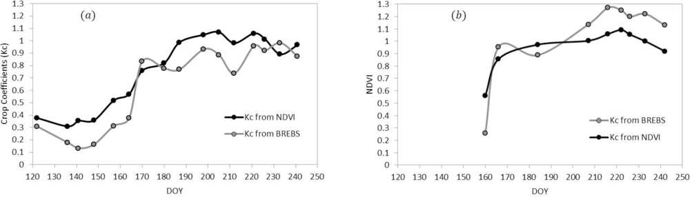
In this section, we present the performance of the NDVI-Kc model (Equation (6)) for maize and soybean fields at the SCAL Bowen-Ratio Energy Balance System (BREBS) site. We used the Mead sites and Cottonwood site in 2007 as the model development dataset, while model validation datasets were used from SCAL in 2006 and 2007. This validation site is independent from the calibration sites, Mead and Cottonwood. The NDVI-Kc regression model (Equation (6)) developed in this study was used to calculate Kc from NDVI values for the SCAL validation data sets for 2006 and 2007. The progression of NDVI and crop coefficient shows the linear relationship. Figure 6 shows the linear regression relationship between the measured crop coefficient and predicted crop coefficient values from the model for year 2006 and 2007.
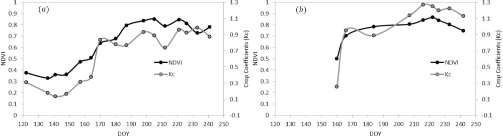
Obviously, the majority of crop coefficient estimates are accurate, with regression analysis near 90% for both fields, where estimates are from Equation (6). The coefficients of determination (r2) between measured and simulated crop coefficients values for 2006 and 2007 were, respectively, about 0.91 and 0.90. The RMSE between measured and predicted crop coefficients by the NDVI-Kc model values were, respectively, about 0.16 and 0.19 for 2006 and 2007 for SCAL. The additional statistical results presented in Table 3 confirm a reasonable performance of the NDVI-Kc model. Figure 7 illustrates the time course of measured and predicted crop coefficients by the NDVI-Kc model for maize and soybean, respectively. However, some discrepancies between measured and predicted crop coefficients by the NDVI-Kc model can still be seen (Figure 7).
3.4. Uncertainties, Errors and Accuracies for NDVI and Crop Coefficient Relationship
Comparison of the normalized difference vegetation index (NDVI) from moderate resolution satellite data (MODIS) and the crop coefficient (Kc) indicate a useful relationship within the limits of the estimated errors or uncertainties. The accuracy of the Kc via remote sensing estimates was ±9% at the 90% confidence level. The Kc from remote sensing accuracy estimates are based on uncertainties associated with input data, resolution and satellite data accuracy. The statistical procedure used to calculate accuracy is explained in the previous section. Our results show that NDVI-Kc models estimate Kc to ±0.2 (see RMSE in Table 3), with the low resolution NDVI estimation. In modeling Kc, it is inevitable that both model and data input will present some uncertainty. Whatever model is used, the errors in the input will propagate to the output of the calculated Kc. However, the NDVI and Kc used in this model calibration and validation are often observed with sufficient accuracy to avoid large errors in the residual. Other independent estimates of Kc from remote sensing are lacking in the literature, so we cannot contrast to the results from other studies. In order to obtain realistic crop coefficient values from remote sensing data, the model inputs and outputs must be correlated. It is critically important to model and evaluate correlations of input variables. Ignoring the correlation between the input parameters (NDVI) will add noise in the model output. Another reason for the errors in the Kc estimation might be due to unknown irrigation schedules and high evaporation, because of precipitation. As the prominent research already suggested, ±10% error prediction of the Kc values is considered to represent levels of ET under pristine growing conditions. In the case above, the inaccuracy of the measurement results is expressed as permissible error. The statistical data shows some minor discrepancies between the observed and estimated Kc (Table 3). The coefficient of determination and RMSE between KcNDVI and observed Kc using BREBS were exceptional low. The Willmott index of agreement is high, 0.93 and 0.84, respectively, for year 2006 and 2007. This is an indication of the accuracy of the model, which suggests it can be used to estimate Kc with different management practices. Biases in the model estimates were consistent over time and on the same order for irrigated and rainfed crops as the NDVI- Kc uncertainty, so that it was concluded that the technique is valuable for estimating the Kc from the remote sensing data.
4. Conclusion
This study developed a simple linear regression model (KcNDVI = 1.457 NDVI – 0.1725) to establish a general relationship between a normalized difference vegetation index (NDVI) from moderate resolution satellite data (MODIS) and the crop coefficient (Kc). Furthermore, because NDVI is specific to the crop at each pixel, Kc is a direct representation of actual crop growth conditions in the field. The crop coefficients were estimated spatially and temporally using the remote sensing model applied to MODIS images taken during the year 2007. Results showed that variations in Kc are well explained by variations in NDVI, especially for well-watered agricultural cropping systems. Kc had a strong relation to NDVI during mid-season periods.
NDVI is an indicator of the density of vegetative cover and plant vigor; therefore, it is not surprising that it captures most of the variation observed in Kc when there is no water stress condition. Validation of the simple regression model yielded an r2 of.90 and an RMSE less than 0.17 for an irrigated maize field at SCAL in NE for two consecutive years (2006 and 2007). The systematic bias (±5%) may be due to wet (2006) and dry (2007) effects on the crop evaporation, not represented in this Kc formulation. The procedure for quantifying crop coefficients from NDVI data presented in this paper should be useful in other regions of the globe to understand regional irrigation water consumption. Biases and uncertainties in the model estimates were consistent over time and of the same order for irrigated and rainfed crops as the NDVI-Kc model, so that it was concluded that the technique is valuable for estimating the Kc from the remote sensing data. We have provided evidence that crop coefficients quantified from remote sensing using this NDVI-Kc equation may be useful for irrigation scheduling, evaluating irrigation/project performance, agricultural water budgets and estimating water use efficiency. The NDVI-Kc model shows promise for use in water conservation in agriculture at the local, regional and continental scales of measurement.
References
- Allen, R.G.; Pereira, L.S.; Raes, D.; Smith, M. Crop Evapotranspiration—Guidelines for Computing Crop Water Requirements—FAO Irrigation and Drainage Paper 56; FAO: Rome, Italy, 1998. [Google Scholar]
- Allen, R.G.; Pereira, L.S.; Smith, M.; Raes, D.; Wright, J.L. The FAO-56 dual crop coefficient method for predicting evaporation from soil and application extensions. J. Irrig. Drain. Eng 2005, 131, 2–13. [Google Scholar]
- Allen, R.G.; Walter, I.A.; Elliot, R.L.; Howell, T.A.; Itenfisu, D.; Jensen, M.E.; Snyder, R.L. The ASCE Standardized Reference Evaportranspiration Equation; American Society of Civil Engineers: Danvers, MA, USA, 2005; p. 59. [Google Scholar]
- Justice, C.O.; Townshend, J.R.G. Special issue on the Moderate Resolution Imaging Spectroradiometer (MODIS): A new generation of land surface monitoring. Remote Sens. Environ 2002, 83, 1–2. [Google Scholar]
- Doorenbos, J.; Pruitt, W.O. Guidelines for Predicting Crop Water Requirements; Irrigation and Drainge Paper 24; FAO: Rome, Italy, 1975. [Google Scholar]
- Kamble, B.; Chemin, Y.H. GIPE in GRASS Raster Addons. Available online: https://svn.osgeo.org/grass/grass-addons/grass6/imagery/gipe/i.vi.grid/description.html (accessed on 1 October 2012).
- Kamble, B.; Irmak, A. Assimilating Remote Sensing-Based ET into SWAP Model for Improved Estimation of Hydrological Predictions. Proceeding of the 2008 IEEE International Geoscience and Remote Sensing Symposium, Boston, MA, USA, 7–11 July 2008; 3. [CrossRef]
- Sellers, P.J. Canopy reflectance, photosynthesis and transpiration. Int. J. Remote Sens 1985, 6, 1335–1372. [Google Scholar]
- Tucker, C.J. Red and photographic infrared linear combinations for monitoring vegetation. Remote Sens. Environ 1979, 8, 127–150. [Google Scholar]
- Boegh, E.; Soegaard, H.; Hanan, N.; Kabat, O.; Lesch, L. A remote sensing study of the NDVI-Ts relationship and the transpiration from sparse vegetation in the Sahel based on high resolution data. Remote Sens. Environ 1998, 69, 224–240. [Google Scholar]
- Hunsaker, D.J.; Pinter, P.J., Jr.; Kimball, B.A. Wheat basal crop coefficients determined by normalized difference vegetation index. Irrig. Sci 2005, 24, 1–14. [Google Scholar]
- Bastiaanssen, W.G.M. SEBAL-based sensible and latent heat fluxes in the irrigated Gediz Basin, Turkey. J. Hydrol 2000, 229, 87–100. [Google Scholar]
- Irmak, S. Nebraska water and energy flux measurement, modeling, and research network (NEBFLUX). Trans. ASABE 2010, 53, 1097–1115. [Google Scholar]
- Jensen, M.E.; Burman, R.D.; Allen, R.G. (Eds.) Evapotranspiration and Irrigation Water Requirements; ASCE: Reston, VA, USA, 1990.
- Bausch, W.C.; Neale, C.M.U. Spectral inputs improve Maize crop coefficients and irrigation scheduling. Trans. ASAE 1989, 32, 1901–1908. [Google Scholar]
- Jayanthi, H.; Neale, C.M.U.; Wright, J.L. Seasonal Evapotranspiration Estimation Using Canopy Reflectance: A Case Study Involving Pink Beans. Proceedings of Remote Sensing and Hydrology 2000, Santa Fe, NM, USA, 2–7 April 2000; pp. 302–305.
- Irmak, A.; Ratcliffe, I.; Ranade, P.; Hubbard, K.; Singh, R.K.; Kamble, B.; Kjaersgaard, J. Estimation of land surface evapotranspiration with a satellite remote sensing procedure. Great Plains Res 2011, 21, 73–88. [Google Scholar]
- Benedetti, R.; Rossinni, P. On the use of NDVI profiles as a tool for agricultural statistics: The case study of wheat yield estimate and forecast in Emilia Romagna. Remote Sens. Environ 1993, 45, 311–326. [Google Scholar]
- Choudhury, B.J.; Ahmed, N.U.; Idso, S.B.; Reginato, R.J.; Daughtry, C.S.T. Relations between evaporation coefficients and vegetation indices studies by model simulations. Remote Sens. Environ 1994, 50, 1–17. [Google Scholar]
- Irmak, A.; Kamble, B. Evapotranspiration data assimilation with genetic algorithms and SWAP model for on-demand irrigation. Irrig. Sci 2009, 28, 101–112. [Google Scholar]
- Hubbard, K.G.; Sivakumar, M.V.K. (Eds.) Automated Weather Stations for Applications in Agriculture and Water Resources Management: Current Use and Future Perspectives. Proceedings of an International Workshop, Lincoln, NE, USA, 6–10 March 2000.
- Allen, R.G.; Clemmens, A.J.; Burt, C.M.; Solomon, K.; O’Halloran, T. Prediction accuracy for projectwide evapotranspiration using crop coefficients and reference evapotranspiration. J. Irrig. Drain. Eng 2005, 131, 24–36. [Google Scholar]
- Gamon, J.A.; Field, C.B.; Goulden, M.; Griffn, K.; Hartley, A.; Joel, G.; Penuelas, J.; Valentini, R. Relationships between NDVI, canopy structure and photosynthesis in three Californian vegetation types. Ecol. Appl 1995, 5, 28–41. [Google Scholar]
- Tasumi, M.; Allen, R.; Trezza, R.; Wright, J. Satellite-Based energy balance to assess within-population variance of crop coefficient curves. J. Irrig. Drain. Eng 2005, 131, 94–109. [Google Scholar]
- Hubbard, K.G. Climatic factors that limit daily evapotranspiration in sorghum. Clim. Res 1992, 2, 73–80. [Google Scholar]
- Baldocchi, D.; Falge, E.; Gu, L.H.; Olson, R.; Hollinger, D.; Running, S.; Anthoni, P.; Bernhofer, C.; Davis, K.; Evans, R.; et al. FLUXNET: A new tool to study the temporal and spatial variability of ecosystem-scale carbon dioxide, water vapor, and energy flux densities. Bull. Am. Meteorol. Soc 2001, 82, 2415–2434. [Google Scholar]
- Verma, S.B.; Dobermann, A.; Cassman, K.G.; Walters, D.T.; Knops, J.M.H.; Arkebauer, T.J.; Suyker, A.E.; Burba, G.G.; Amos, B.; Yang, H.S. Annual carbon dioxide exchange in irrigated and rainfed maize based agro-ecosystems. Agric. For. Meteorol 2005, 131, 77–96. [Google Scholar]
- Singh, R.; Irmak, A. Estimation of crop coefficients using satellite remote sensing. J. Irrig. Drain. Eng 2009, 135, 597–608. [Google Scholar]
- Hargreaves, G.H.; Samani, Z.A. Reference crop evapotranspiration from temperature. Appl. Eng. Agric 1985, 1, 96–99. [Google Scholar]
- Hargreaves, G.H.; Allen, R.G. History and evaluation of Hargreaves evapotranspiration equation. J. Irrig. Drain. Eng 2003, 129, 53–63. [Google Scholar]
- Duffie, J.A.; Beckman, W.A. Solar Engineering of Thermal Processes; John Wiley & Sons: New York, NY, USA, 1980. [Google Scholar]
- Rouse, J.W.; Haas, R.H.; Schell, J.A.; Deering, D.W. Monitoring Vegetation Systems in the Great Plains with ERTS, Proceedings of Third ERTS Symposium, Washington, DC, USA, 10–14 December 1973; 1, pp. 309–317.
- Gitelson, A.; Vina, A.; Masek, J.; Verma, S.; Suyker, A. Synoptic monitoring of gross primary productivity of maize using Landsat data. IEEE Geosci. Remote Sens. Lett 2008, 5, 133–137. [Google Scholar]
Figure 1.
Seasonal progression of weather (maximum (red) and minimum (gray) temperature, precipitation (blue)) data at model calibration sites: (a) Mead Irrigated Rotation, NE, USA (Year 2007); (b) Mead Irrigated, NE, USA (Year 2007); (c) Mead Rainfed, NE, USA (Year 2007); (d)Cottonwood, SD, USA (Year 2007).

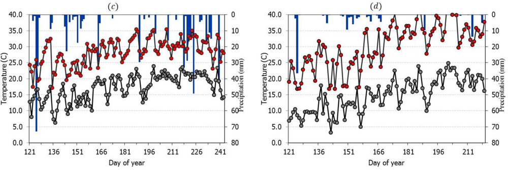
Figure 2.
Seasonal progression of weather (maximum (red) and minimum (gray) temperature, precipitation (blue)) data at model validation sites (a) South Central Agricultural Laboratory (Year 2007), (b) South Central Agricultural Laboratory (Year 2006).
Figure 2.
Seasonal progression of weather (maximum (red) and minimum (gray) temperature, precipitation (blue)) data at model validation sites (a) South Central Agricultural Laboratory (Year 2007), (b) South Central Agricultural Laboratory (Year 2006).
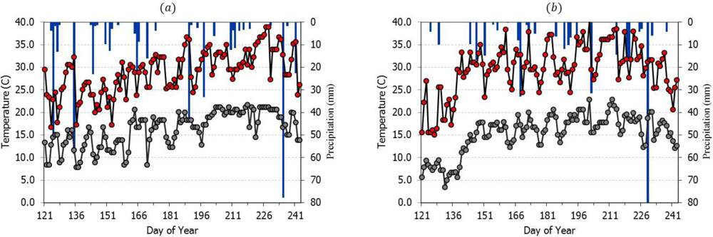
Figure 3.
Seasonal progression of NDVI and Kc at model calibration sites: (a) Mead Irrigated Rotation, NE, USA (Year 2007); (b) Mead Irrigated, NE, USA (Year 2007); (c) Mead Rainfed, NE, USA (Year 2007); (d) Cottonwood, SD, USA (Year 2007).
Figure 3.
Seasonal progression of NDVI and Kc at model calibration sites: (a) Mead Irrigated Rotation, NE, USA (Year 2007); (b) Mead Irrigated, NE, USA (Year 2007); (c) Mead Rainfed, NE, USA (Year 2007); (d) Cottonwood, SD, USA (Year 2007).
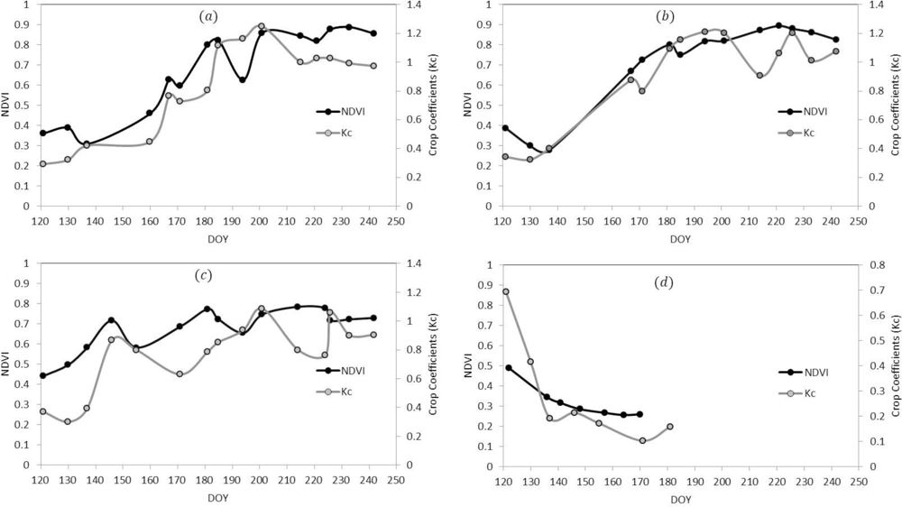
Figure 4.
Seasonal progression of NDVI and Kc at model validation sites: (a) South Central Agricultural Laboratory (Year 2006); (b) South Central Agricultural Laboratory (Year 2007).
Figure 4.
Seasonal progression of NDVI and Kc at model validation sites: (a) South Central Agricultural Laboratory (Year 2006); (b) South Central Agricultural Laboratory (Year 2007).

Figure 5.
Relationship between Terra-MODIS NDVI and AmeriFlux measured crop coefficients under irrigated and rainfed crop condition.
Figure 5.
Relationship between Terra-MODIS NDVI and AmeriFlux measured crop coefficients under irrigated and rainfed crop condition.
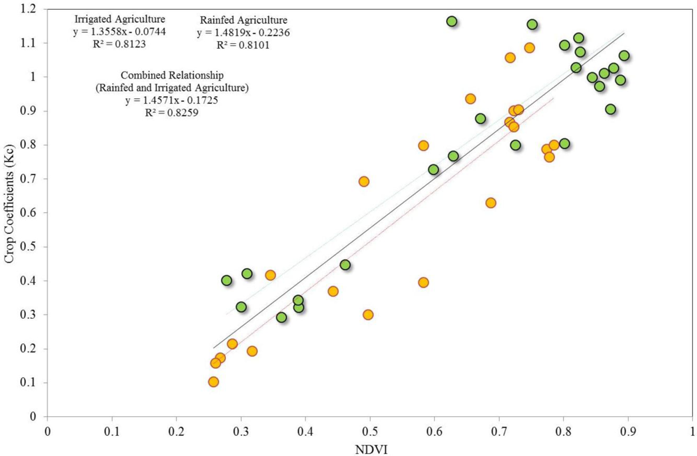
Figure 6.
Validation of the NDVI-Kc model: (a) irrigated maize for growing season in 2006 and (b) soybean for 2007 in SCAL data. The graph depicts regression scatter plots of estimated vs. observed crop coefficient.
Figure 6.
Validation of the NDVI-Kc model: (a) irrigated maize for growing season in 2006 and (b) soybean for 2007 in SCAL data. The graph depicts regression scatter plots of estimated vs. observed crop coefficient.

Figure 7.
Seasonal progression of measured Kc and estimated Kc: (a) irrigated maize for growing season in 2006 and (b) soybean for 2007 in SCAL data.
Figure 7.
Seasonal progression of measured Kc and estimated Kc: (a) irrigated maize for growing season in 2006 and (b) soybean for 2007 in SCAL data.

Table 1.
Vegetation type, geographical location and cropping patterns of the study sites used to develop the normalized difference vegetation index (NDVI)-crop coefficient (Kc) relationship.
| Year | Name | Latitude | Longitude | Elevation (m) | Canopy Height | Vegetation Type | Crop |
|---|---|---|---|---|---|---|---|
| 2007 | Mead Irrigated Rotation | 41.1649 | −96.4701 | 362 | 1.83 m | Agriculture (maize-soybean rotation) | Maize |
| 2007 | Mead Rainfed | 41.1797 | −96.4396 | 363 | 1.71 m | Agriculture (maize) | Maize |
| 2007 | Mead Irrigated Continuous | 41.1651 | −96.4766 | 361 | 2.90 m | Agriculture (continuous maize) | Maize |
| 2007 | Cottonwood | 43.95 | −101.8466 | 744 | 20–40 cm | Grassland/range | Grass |
| 2007 | South-Central Agricultural Laboratory, Clay Center | 40.56667 | −98.1333 | 552 | N/A | Agriculture Soybean/maize | Maize |
| 2006 | South-Central Agricultural Laboratory, Clay Center | 40.56667 | −98.133333 | 552 | N/A | Agriculture (Soybean/maize) | Soybean |
| Sites | Mean | Max | Min | Standard Deviation | ||||
|---|---|---|---|---|---|---|---|---|
| NDVI | Kc | NDVI | Kc | NDVI | Kc | NDVI | Kc | |
| Cottonwood, SD, USA | 0.318 | 0.279 | 0.490 | 0.693 | 0.257 | 0.103 | 0.083 | 0.208 |
| Mead Irrigated Rotation, NE, USA | 0.676 | 0.822 | 0.822 | 5.302 | 0.309 | 0.293 | 0.209 | 0.316 |
| Mead Irrigated, NE, USA | 0.706 | 0.905 | 0.894 | 1.212 | 0.277 | 0.323 | 0.218 | 0.323 |
| Mead Rainfed, NE, USA | 0.676 | 0.763 | 0.785 | 1.086 | 0.442 | 0.300 | 0.104 | 0.240 |
| SCAL-2007 | 0.767 | 1.034 | 0.866 | 1.271 | 0.502 | 0.257 | 0.111 | 0.320 |
| SCAL-2006 | 0.636 | 0.635 | 0.852 | 0.984 | 0.330 | 0.133 | 0.200 | 0.323 |
| Statistical Index | 2006 | 2007 |
|---|---|---|
| Mean error | 0.12 | −0.09 |
| Mean absolute error | 0.14 | 0.17 |
| Mean square error | 0.02 | 0.03 |
| Root mean square error | 0.16 | 0.19 |
| Ratio of standard deviations | 0.9 | 0.51 |
| Nash-Sutcliffe efficiency | 0.75 | 0.62 |
| Willmott index of agreement | 0.93 | 0.84 |
| Coefficient of persistence | −0.01 | 0.62 |
| Pearson product-moment correlation coefficient | 0.95 | 0.95 |
| Coefficient of determination | 0.91 | 0.90 |
Share and Cite
MDPI and ACS Style
Kamble, B.; Kilic, A.; Hubbard, K. Estimating Crop Coefficients Using Remote Sensing-Based Vegetation Index. Remote Sens. 2013, 5, 1588-1602. https://doi.org/10.3390/rs5041588
AMA Style
Kamble B, Kilic A, Hubbard K. Estimating Crop Coefficients Using Remote Sensing-Based Vegetation Index. Remote Sensing. 2013; 5(4):1588-1602. https://doi.org/10.3390/rs5041588
Chicago/Turabian StyleKamble, Baburao, Ayse Kilic, and Kenneth Hubbard. 2013. "Estimating Crop Coefficients Using Remote Sensing-Based Vegetation Index" Remote Sensing 5, no. 4: 1588-1602. https://doi.org/10.3390/rs5041588