A Vegetation Index to Estimate Terrestrial Gross Primary Production Capacity for the Global Change Observation Mission-Climate (GCOM-C)/Second-Generation Global Imager (SGLI) Satellite Sensor


Abstract
:1. Introduction
2. Methods
2.1. VI for Estimating the Maximum Rate of Low-Stress GPP
2.2. Selection of Vegetation Indices (VIs)
- The NDVI[55] is the most widely used index for many vegetation applications. However, the NDVI has a saturation problem with very dense vegetation.
- The enhanced VI (EVI) [56] is an improved VI that accounts for the effects of residual atmospheric contamination and soil background. The EVI reduces the saturation problem in various canopies.
- The modified NDVI (mNDVI) [57] was developed to eliminate the effects of surface reflectance by incorporating the blue band. This VI is more strongly correlated with total chlorophyll and eliminates the effect of surface reflectance.
- The green and red ratio VI (GRVI) [58] was proposed as an index to monitor the photosynthetically active biomass of plant canopies. The GRVI is calculated from the visible green and red reflectance.
- The simple ratio index (SR) [59] is probably the first index and is the most commonly used to derive LAI for a forest canopy.
- The green NDVI (GNDVI) [50] is a better VI at a higher LAI and is good at detecting chlorophyll. The GNDVI can detect a wider range of chlorophyll compared to the NDVI.
- The green chlorophyll index (CIgreen)[25] is sensitive to a wide range of chlorophyll variation. CIgreen can estimate canopy chlorophyll content under a wide range of canopy conditions.
2.3. Data Sets
2.3.1. Leaf-Scale Data Set
2.3.2. Canopy-Scale Data Set
2.3.3. Satellite-Scale Data Set: EC Flux Data and MODIS Spectral Reflectance of Seven Plant Functional Types
2.4. Data Processing
2.4.1. Reflectance Data Process
2.4.2. Photosynthetic Capacity Calculation Processes
EC Flux Data Process for Selection of Low-Stress Data
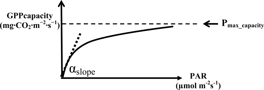
Pmax_capacity Calculation
2.5 Validation of the VI
3. Results
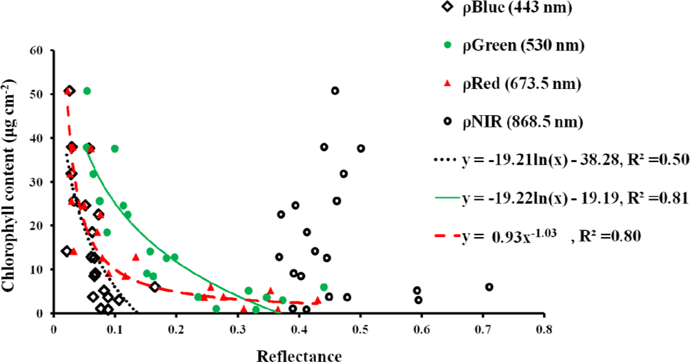
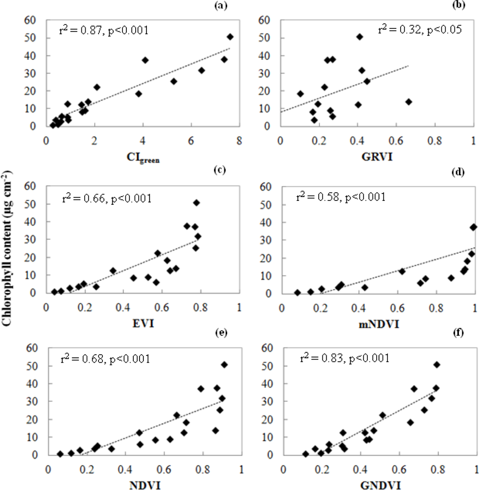
3.1. Leaf Scale: Relationship between VIs and Chlorophyll Content
3.2. GPPcapacity Selection Criteria
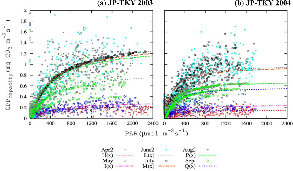
3.3. Canopy and Satellite Scales: Results for Broadleaf Deciduous Temperate Trees at JP-TKY
3.3.1. Pmax_capacity of the Light-Response Curve from EC Flux Data
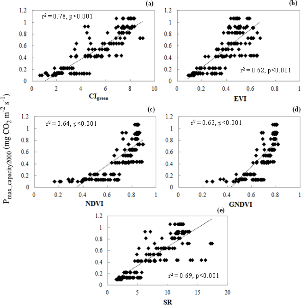
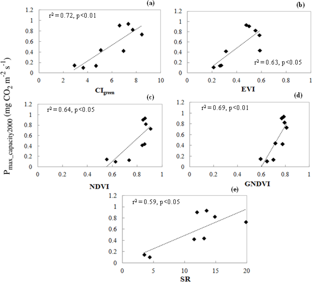
3.3.2. Relationship of VIs and Pmax_capacity2000
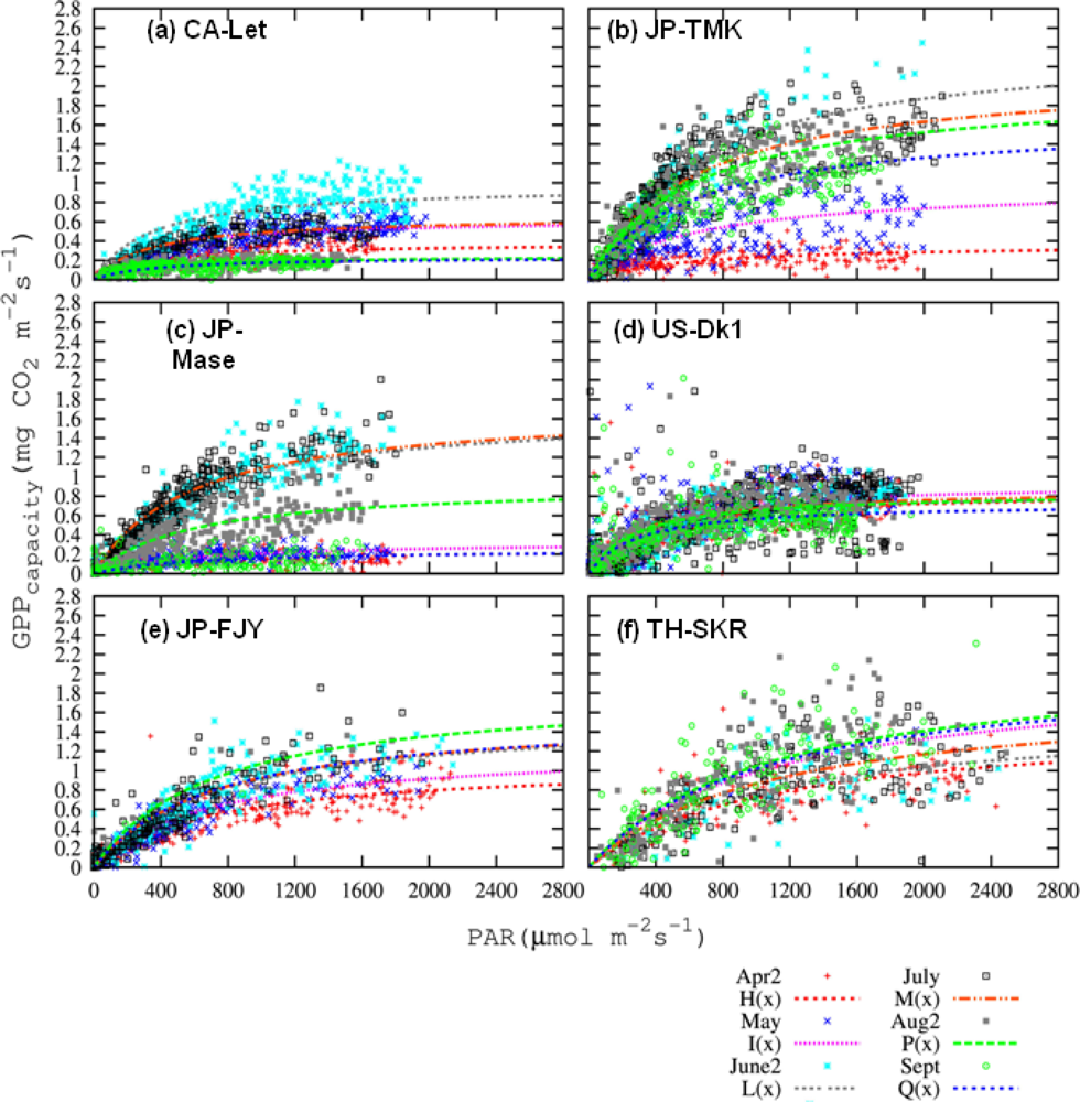
3.4. Satellite-Scale: Results for Various Plant Functional Types
3.4.1. Pmax_capacity of the Light-Response Curve from EC Flux Data
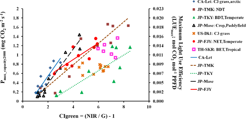
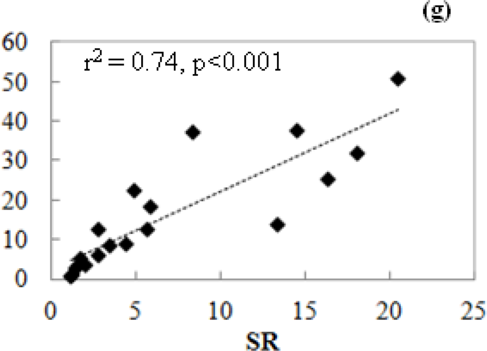
3.4.2. Relationships of CIgreen and Pmax_capacity2000
3.4.3. Validation of CIgreen
4. Discussion
5. Conclusion
Acknowledgments
References
- Zhao, M.; Running, S.W. Drought-induced reduction in global terrestrial net primary production from 2000 through 2009. Science 2010, 329, 940–943. [Google Scholar]
- Tanaka, K.; Okamura, Y.; Amano, T.; Hiramatsu, M.; Shiratama, K. Development status if the Second-generation Global Imager (SGLI) On GCOM-C1. Presented at SPIE Europe Security + Defence, Berlin, Germany, 31 August–3 September 2009.
- Monteith, J. Solar radiation and production in tropical ecosystems. J. Appl. Ecol 1972, 9, 747–766. [Google Scholar]
- Heinsch, F.A.; Zhao, M.; Running, S.W.; Kimball, J.S.; Nemani, R.R.; Davis, K.J.; Bolstad, P.V.; Cook, B.D.; Desai, A.R.; Ricciuto, D.M.; et al. Evaluation of remote sensing based terrestrial productivity from MODIS using tower eddy flux network observations. IEEE Trans. Geosci. Remote Sens 2006, 44, 1908–1925. [Google Scholar]
- Wu, C.; Chen, J.M.; Desai, A.R.; Hollinger, D.Y.; Arain, M.A.; Margolis, H.A.; Gough, C.M.; Staebler, R.M. Remote sensing of canopy light use efficiency in temperate and boreal forests of North America using MODIS imagery. Remote Sens. Environ 2012, 118, 60–72. [Google Scholar]
- Coops, N.C.; Hilker, T.; Hall, F.G.; Nichol, C.J.; Drolet, G.G. Estimation of light-use efficiency of terrestrial ecosystems from space: A status report. BioScience 2010, 60, 788–797. [Google Scholar]
- Potter, C.S.; Randerson, J.T.; Field, C.B.; Matson, P.A.; Vitousek, P.M.; Mooney, H.A.; Klooster, S.A. Terrestrial ecosystem production: A process model based on global satellite and surface data. Glob. Biogeochem. Cy 1993, 7, 811–841. [Google Scholar]
- Cramer, W.; Kicklighter, D.W.; Bondeau, A.; Moore, B., III; Churkina, G.; Nemry, B.; Ruimy, A.; Schloss, A.L. Participants of the Potsdam NPP Model Intercomparison. Comparing global models of terrestrial net primary production (NPP): Overview and key results. Global Change Biol 1999, 5, 1–15. [Google Scholar]
- Running, S.W.; Nemani, R.R.; Heinsch, F.A.; Zhao, M.; Reeves, M.; Hashimoto, H.A. Continuous satellite-derived measure of global terrestrial primary production. BioScience 2004, 54, 547–560. [Google Scholar]
- Sasai, T.; Okamoto, K.; Hiyama, T.; Yamaguchi, Y. Comparing terrestrial carbon fluxes from the scale of a flux tower to the global scale. Ecol. Model 2007, 208, 135–144. [Google Scholar]
- Beer, C.; Reichstein, M.; Tomelleri, E.; Ciais, P.; Jung, M.; Carvalhais, N.; Rödenbeck, C.; Arain, M.A.; Baldocchi, D.; Bonan, G.B.; et al. Terrestrial gross carbon dioxide uptake: Global distribution and covariation with climate. Science 2010, 329, 834–838. [Google Scholar]
- Jung, M.; Reichstein, M.; Bondeau, A. Towards global empirical upscaling of FLUXNET eddy covariance observation of a model tree ensemble approach using a biosphere model. Biogeoeciences 2009, 6, 2001–2013. [Google Scholar]
- Zhang, F.; Chen, J.M.; Chen, J.; Gough, C.M.; Martin, T.A.; Dragoni, D. Evaluating spatial and temporal patterns of MODIS GPP over the conterminous U.S. against flux measurements and a process model. Remote Sens. Environ 2012, 124, 717–729. [Google Scholar]
- Chen, J.M.; Liu, J.; Cihlar, J.; Guolden, M.L. Daily canopy photosynthesis model through temporal and spatial scaling for remote sensing applications. Ecol. Model 1999, 124, 99–119. [Google Scholar]
- Ryu, Y.; Baldocchi, D.D.; Kobayashi, H.; Ingen, C.V.; Li, J.; Black, A.T.; Beringer, J.; Gorsel, E.V.; Knohl, A.; Law, B.E.; Roupsard, O. Integration of MODIS land and atmosphere products with a coupled-process model to estimate gross primary productivity and evapotranspiration from 1 km to global scales. Glob. Biogeochem. Cy. 2011, 25, GB4017. [Google Scholar]
- Muraoka, H.; Koizumi, H. Photosynthetic and structural characteristics of canopy and shrub trees in a cool-temperate deciduous broadleaved forest: Implication to the ecosystem carbon gain. Agric. Forest Meteorol 2005, 134, 39–59. [Google Scholar]
- Muraoka, H.; Saigusa, N.; Nasahara, K.N.; Noda, H.; Yoshino, J.; Saitoh, T.M.; Nagai, S.; Murayama, S.; Koizumi, H. Effects of seasonal and interannual variations in leaf photosynthesis and canopy leaf area index on gross primary production of a cool-temperate deciduous broadleaf forest in Takayama, Japan. J. Plant Res 2010, 123, 563–576. [Google Scholar]
- Houborg, R.; Anderson, M.C.; Norman, J.M.; Wilson, T.; Meyers, T. Intercomparison of a ‘bottom-up’ and ‘top-down’ modelling paradigm for estimating carbon and energy fluxes over a variety of vegetative regimes across the U.S. Agric. Forest Meteorol 2009, 149, 2162–2182. [Google Scholar]
- Reichstein, M.; Tenhunen, J.; Roupsard, O.; Ourcival, J.M.; Rambal, S.; Miglietta, F.; Peressotti, A.; Pecchiari, M.; Tirone, G.; Valentini, R. Inverse modeling of seasonal drought effects on canopy CO2/H2O exchange in three Mediterranean ecosystems. J. Geophys. Res 2003, 108, 4726–4742. [Google Scholar]
- Shibayama, M.; Akiyama, T.A. A spectroradiometer for field use: 6. Radiometric estimation for chlorophyll index of rice canopy. Jpn. J. Crop Sci 1986, 55, 433–438. [Google Scholar]
- Gamon, J.A.; Serrano, L.; Surfus, J.S. The photochemical reflectance index: an optical indicator of photosynthetic radiation use efficiency across species, functional types and nutrient levels. Oecologia 1997, 112, 492–501. [Google Scholar]
- Inoue, Y.; Peñuelas, J.; Miyata, A.; Mano, M. Normalized difference spectral indices for estimating photosynthetic efficiency and capacity at a canopy scale derived from hyperspectral and CO2 flux measurements in rice. Remote Sens. Environ 2008, 112, 156–172. [Google Scholar]
- Gitelson, A.A.; Merzlyak, M.N. Quantitative estimation of chlorophyll-a using reflectance spectra: Experiments with autumn chestnut and maple leaves. J. Photochem. Photobiol. B: Biol 1994, 22, 247–252. [Google Scholar]
- Gitelson, A.; Merzlyak, M.N. Signature analysis of leaf reflectance spectra: Algorithm development for remote sensing of chlorophyll. J. Plant Physiol 1996, 148, 494–500. [Google Scholar]
- Gitelson, A.; Merzlyak, M. Remote estimation of chlorophyll content in higher plant leaves. Int. J. Remote Sens 1997, 18, 291–298. [Google Scholar]
- Gitelson, A.A.; Gritz, Y.; Merzlyak, M.N. Relationships between leaf chlorophyll content and spectral reflectance and algorithms for non-destructive chlorophyll assessment in higher plant leaves. J. Plant Physiol 2003, 160, 271–282. [Google Scholar]
- Gitelson, A.A.; Viña, A.; Arkebauer, T.J.; Rundquist, D.C.; Keydan, G.; Leavitt, B. Remote estimation of leaf area index and green leaf biomass in maize canopies. Geophys. Res. Lett 2003, 30, 1248–1252. [Google Scholar]
- Gitelson, A.A.; Viña, A.; Rundquist, D.C.; Ciganda, V.; Arkebauer, T.J. Remote estimation of canopy chlorophyll content in crops. Geophys. Res. Lett 2005, 32, L08403–L08407. [Google Scholar]
- Sims, D.A.; Luo, H.; Hastings, S.; Oechel, W.C.; Rahman, A.F.; Gamon, J.A. Parallel adjustments in vegetation greenness and ecosystem CO2 exchange in response to drought in a Southern California chaparral ecosystem. Remote Sens. Environ 2006, 103, 289–303. [Google Scholar]
- Horler, D.N.H.; Dockray, M.; Barber, J. The red edge of plant leaf reflectance. Int. J. Remote Sens 1983, 4, 273–288. [Google Scholar]
- Dash, J.; Curran, P.J. MTCI: The MERIS Teresrial Chlorophyll Index. Proceeding of MERIS User Workshop, Frascati, Italy, 10–13 November 2003.
- Haboudane, D.; Miller, J.R.; Tremblay, N.; Zarco-Tejada, P.J.; Dextrase, L. Integrated narrow-band vegetation indices for prediction of crop chlorophyll content for application to precision agriculture. Remote Sens. Environ 2002, 81, 416–426. [Google Scholar]
- Huete, A.R. A soil adjusted vegetation index (SAVI). Remote Sens. Environ 1988, 25, 295–309. [Google Scholar]
- Rondeaux, G.; Steven, M.; Baret, F. Optimization of soil-adjusted vegetation indices. Remote Sens. Environ 1996, 55, 95–107. [Google Scholar]
- Daughtry, C.S.T.; Walthall, C.L.; Kim, M.S.; de Colstrum, E.B.; McMurtrey, J.E., III. Estimating corn leaf chlorophyll concentration from leaf and canopy reflectance. Remote Sens. Environ 2000, 74, 229–239. [Google Scholar]
- Wu, C.; Niu, Z.; Tang, Q.; Huang, W. Estimating chlorophyll content from hyperspectral vegetation indices: Modeling and validation. Agric. Forest Meteorol 2008, 148, 1230–1241. [Google Scholar]
- Gitelson, A.A.; Viña, A.; Verma, S.; Rundquist, D.C.; Arkebauer, T.J.; Keydan, G.; Leavitt, B.; Ciganda, V.; Burba, G.G.; Suyker, A.E. Relationship between gross primary production and chlorophyll content in crops: Implications for the synoptic monitoring of vegetation productivity. J. Geophys. Res. 2006, 111, D08S11. [Google Scholar]
- Wu, C.; Niu, Z.; Tang, Q.; Huang, W.; Rivard, B.; Feng, J. Remote estimation of gross primary production in wheat using chlorophyll-related vegetation indices. Agric. Forest Meteorol 2009, 149, 1015–1021. [Google Scholar]
- Wu, C.; Wang, L.; Niu, Z.; Gao, S.; Wu, M.Q. Nondestructive estimation of canopy chlorophyll content using Hyperion and Landsat/TM images. Int. J. Remote Sens 2010, 31, 2159–2167. [Google Scholar]
- Wu, C.; Niu, Z.; Gao, S. The potential of the satellite derived green chlorophyll index for estimating midday light use efficiency in maize, coniferous forest and grassland. Ecol. Indic 2012, 14, 66–73. [Google Scholar]
- Gitelson, A.A.; Peng, Y.; Masek, J.G.; Rundquist, D.C.; Verma, S.; Suyker, A.; Baker, J.M.; Hatfield, J.L.; Meyers, T. Remote estimation of crop gross primary production with Landsat data. Remote Sens. Environ 2012, 121, 404–414. [Google Scholar]
- Wu, C.; Chen, J.M.; Huang, N. Predicting gross primary production from the enhanced vegetation index and photosynthetically active radiation: Evaluation and calibration. Remote Sens. Environ 2011, 115, 3424–3435. [Google Scholar]
- Xiong, Y.A. Study on Algorithm for Estimation of Global Terrestrial Net Primary Production using Satellite Sensor Data.
- Furumi, S.; Xiong, Y.; Fujiwara, N. Establishment of an Algorithm to Estimate Vegetation Photosynthesis by Pattern Decomposition Using Multi-Spectral Data. J. Remote Sens. Soc. Jpn 2005, 25, 47–59. [Google Scholar]
- Muramatsu, K.; Furumi, S.; Chen, L.; Xiong, Y.; Daigo, M. Estimation and Validation of Net Primary Production of Vegetation using ADEOS-II/GLI data Global Mosaic and 250-m Spatial Resolution Data. J. Remote Sens. Soc. Jpn 2009, 29, 114–123. [Google Scholar]
- Ide, R.; Nakaji, T.; Oguma, H. Assessment of canopy photosynthetic capacity and estimation of GPP by using spectral vegetation indices and the light–response function in a larch forest. Agric. Forest Meteorol 2010, 150, 389–398. [Google Scholar]
- Sellers, P.J.; Berry, J.A.; Collatz, G.J.; Field, C.B.; Hall, F.G. Canopy reflectance, photosynthesis, and transpiration. III. A reanalysis using improved leaf models and a new canopy integration scheme. Remote Sens. Environ 1992, 42, 187–216. [Google Scholar]
- Taiz, L.; Zeiger, E. Photosynthesis: The Carbon Reactions. In Plant Physiology, 4th ed.; Chapter 8; Sinauer Associates, Inc: Sunderland, MA, USA, 2006. [Google Scholar]
- Jones, H.G.; Vaugha, R.A. Use of Spectral Information for Sensing Vegetation Properties and for Image Classification. In Remote Sensing of Vegetation: Principles, Techniques, and Applications; Chapter 7; Oxford University Press: New York, NY, USA, 2010; pp. 169–170. [Google Scholar]
- Gitelson, A. A.; Kaufman, Y.J.; Merzlyak, M.N. Use of a green channel in remote sensing of global vegetation from EOS-MODIS. Remote Sens. Environ 1996, 58, 289–298. [Google Scholar]
- Nagai, S.; Saigusa, N.; Muraoka, H.; Nasahara, K.N. What makes the satellite-based EVI–GPP relationship unclear in a deciduous broad-leaved forest? Ecol. Res 2010, 25, 359–365. [Google Scholar]
- Lambers, H.; Chapin, FS, III; Pons, TL. Plant Physiological Ecology, 2nd ed.; Springer: New York, NY, USA, 2008; p. 27. [Google Scholar]
- Ono, K.; Hashimoto, H.; Katoh, S. Changes in the number and size of chloroplasts during senescence of primary leaves of wheat grown under different conditions. Plant Cell Physiol 1995, 36, 9–17. [Google Scholar]
- Oguchi, R.; Hikosaka, K.; Hirose, T. Does the photosynthetic light-acclimation need change in leaf anatomy? Plant Cell Environ 2003, 26, 505–512. [Google Scholar]
- Rouse, J.W.; Haas, R.H.; Deering, D.W.; Schell, J.A. Monitoring the Vernal Advancement and Retro Gradation (Green Wave Effect) of Natural Vegetation; Final Report; Remote Sensing Center, Texas A&M University: College Station, TX, USA, 1974. [Google Scholar]
- Huete, A.; Didan, K.; Miura, T.; Rodriguez, E.P.; Gao, X.; Ferreira, L.G. Overview of the radiometric and biophysical performance of the MODIS vegetation indices. Remote Sens. Environ 2002, 83, 195–213. [Google Scholar]
- Sims, D.A.; Gamon, J.A. Relationships between leaf pigment content and spectral reflectance across a wide range of species, leaf structures and developmental stages. Remote Sens. Environ 2002, 81, 337–354. [Google Scholar]
- Tucker, C.J. Red and photographic infrared linear combinations for monitoring vegetation. Remote Sens. Environ 1979, 8, 127–150. [Google Scholar]
- Jordan, C.F. Derivation of leaf area index from quality of light on the forest floor. Ecology 1969, 50, 663–666. [Google Scholar]
- Furumi, S.; Hayashi, A.; Muramatsu, K.; Fujiwara, N. Relation between vegetation vigor and a new vegetation index based on pattern decomposition method. J. Remote Sens. Soc. Jpn 1998, 18, 17–34. [Google Scholar]
- Nishida, K. Phenological Eyes Network (PEN): A validation network for remote sensing of the terrestrial ecosystems. Asia-Flux Newsletter 2007, 21, 9–13. [Google Scholar]
- Bonan, G. A Land Surface Model (LSM version 1.0) for Ecological, Hydrological, and Atmospheric Studies: Technical Description and User’s Guide; NCAR: Boulder, CO, USA, 1996. [Google Scholar]
- Forestry and Forest Products Research Institute. FFPRI FluxNet Database, 2010. Available online: http://www.ffpri.affrc.go.jp/labs/flux/index.html (accessed on 14 November 2012).
- The NASA-developed Earth Observing System (EOS) Clearinghouse (ECHO). Available online: http://reverb.echo.nasa.gov/reverb/#utf8=%E2%9C%93&spatial_map=satellite&spatial_type=rectangle (accessed on 14 November 2012).
- Reichstein, M.; Falge, E.; Baldocchi, D.; Papale, D.; Aubinet, M.; Berbigier, P.; Bernhofer, C.; Buchmann, N.; Gilmanov, T.; Granier, A.; et al. On the separation of net ecosystem exchange into assimilation and ecosystem respiration: review and improved algorithm. Global Change Biol 2005, 11, 1424–1439. [Google Scholar]
- Baldocchi, D.; Falge, E.; Wilson, K. A spectral analysis of biosphere–atmosphere trace gas flux densities and meteorological variables across hour to multi-year time scales. Agric. Forest Meteorol 2001, 107, 1–27. [Google Scholar]
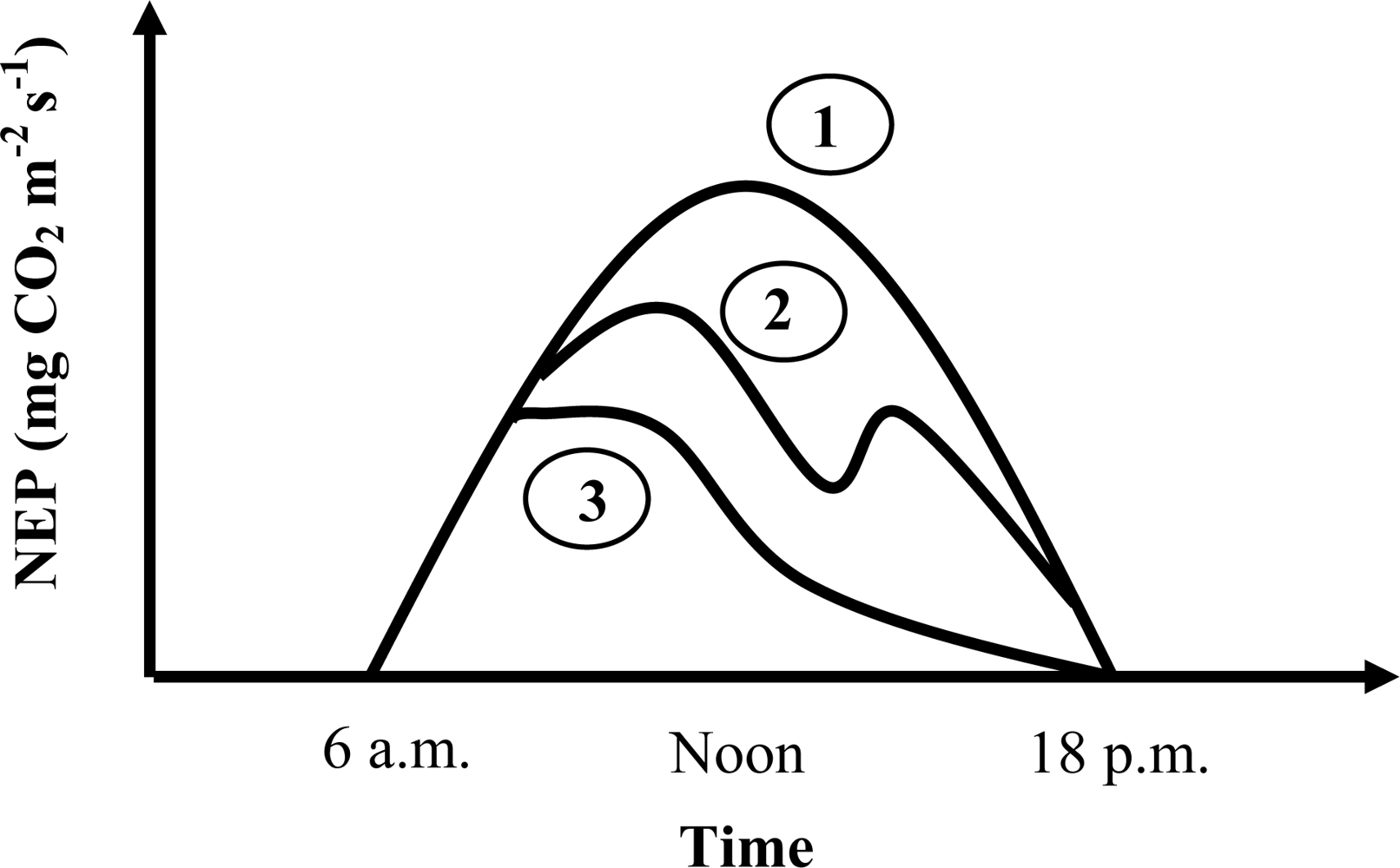
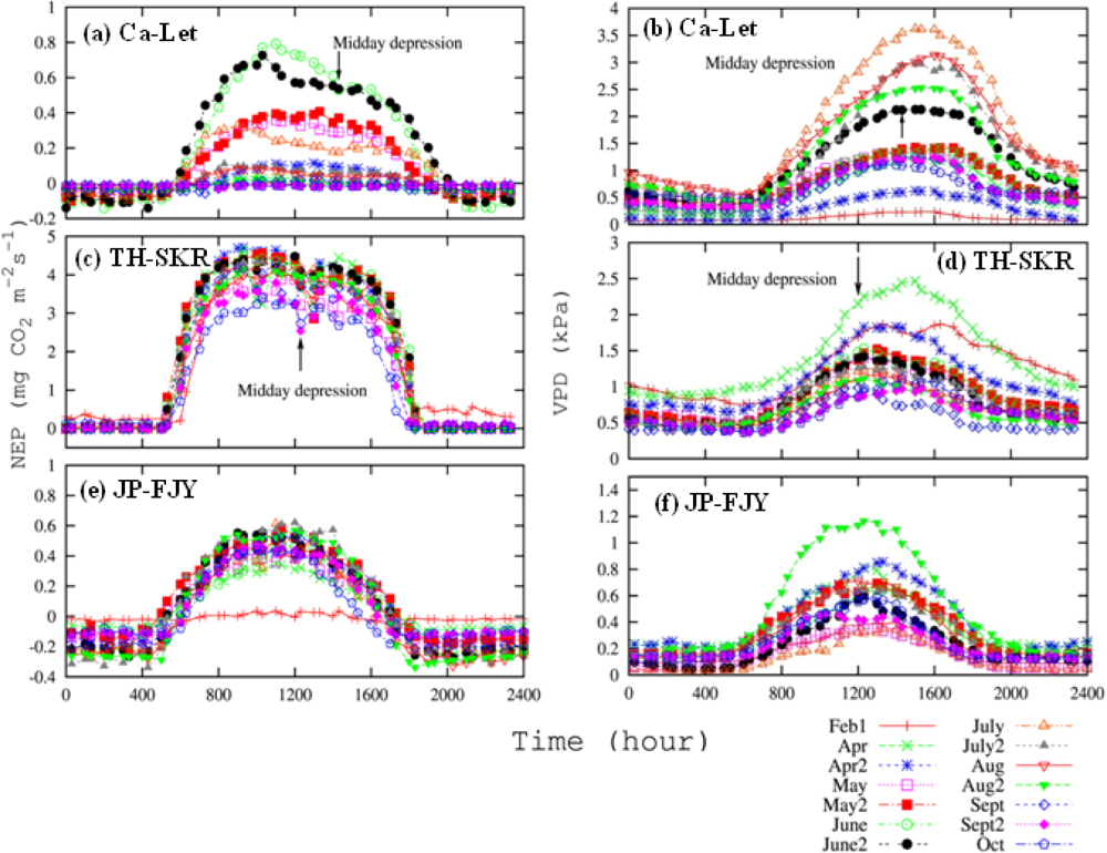
- Pathre, U.; Sinha, A.K.; Shirke, P.A.; Sane, P.V. Factors determining the midday depression of photosynthesis in trees under monsoon climate. Trees 1998, 12, 472–481. [Google Scholar]
- Pessarakli, M. Handbook of Photosynthesis, 2nd ed.; CRC Press: Boca Raton, FL, USA, 2005; p. 287. [Google Scholar]
- Thomas, J.R.; Gausman, H.W. Leaf reflectance vs. leaf chlorophyll and carotenoid concentrations for eight crops. Agron. J 1977, 69, 799–802. [Google Scholar]
- Chappelle, E.W.; Kim, M.S.; McMurtrey, J.E., III. Ratio analysis of reflectance spectra (RARS): An algorithm for the remote estimation of the concentrations of chlorophyll A, chlorophyll B, and carotenoids in soybean leaves. Remote Sens. Environ 1992, 39, 239–247. [Google Scholar]
- Gitelson, A.A.; Chivkunova, O.B.; Merzlyak, M. N. Nondestructive estimation of anthocyanins and chlorophylls in anthocyanic leaves. Am. J. Bot 2009, 96, 1861–1868. [Google Scholar]
- Datt, B. Remote sensing of chlorophyll a, chlorophyll b, chlorophyll a+b, and total carotenoid content in Eucalyptus leaves. Remote Sens. Environ 1998, 66, 111–121. [Google Scholar]
- Buschman, C.; Nagel, E. In vivo spectroscopy and internal optics of leaves as a basis for remote sensing of vegetation. Int. J. Remote Sens 1993, 14, 711–722. [Google Scholar]
- Datt, B. A new reflectance index for remote sensing of chlorophyll content in higher plants: Tests using Eucalyptus leaves. J. Plant Physiol 1999, 154, 30–36. [Google Scholar]
- Yoder, B.J.; Waring, R.H. The normalized difference vegetation index of small Douglas-fir canopies with varying chlorophyll concentrations. Remote Sens. Environ 1994, 49, 81–91. [Google Scholar]
- Gilmanov, T.G.; Tieszen, L.L.; Wylie, B.K.; Flanagan, L.B.; Frank, A.B.; Haferkamp, M.R.; Meyers, T.P.; Morgan, J.A. Integration of CO2 flux and remotely-sensed data for primary production and ecosystem respiration analyses in the Northern Great Plains: Potential for quantitative spatial extrapolation. Global Ecol. Biogeogr 2005, 14, 271–292. [Google Scholar]
- Saigusa, N.; Yamamoto, S.; Hirata, R.; Ohtani, Y.; Ide, R.; Asanuma, J.; Gamo, M.; Hirano, T.; Kondo, H.; Kosugi, Y.; Li, S.G.; Nakai, Y.; Takagi, K.; Tani, M.; Wang, H. Temporal and spatial variations in the seasonal patterns of CO2 flux in boreal, temperate, and tropical forests in East Asia. Agric. Forest Meteorol 2008, 148, 700–713. [Google Scholar]
- Saito, M.; Maksyutov, S.; Hirata, R.; Richardson, A.D. An empirical model simulating diurnal and seasonal CO2 flux for diverse vegetation types and climate conditions. Biogeosciences 2009, 6, 585–599. [Google Scholar]
- Takeda, T.; Yajima, M. An improvement of semiempirical method for estimating the total photosynthesis of the crop population: I. On light-photosynthesis curve of rice leaves (in Japanese). Jpn. J. Crop Sci 1975, 44, 343–349. [Google Scholar]
- Ruimy, A.; Javis, P.G.; Baldocchi, D.D.; Saugier, B. CO2 fluxes over plant canopies and solar radiation: a review. Adv. Ecol. Res 1995, 26, 1–69. [Google Scholar]
- Xiao, X. Light absorption by leaf chlorophyll and maximum light use efficiency. IEEE Trans. Geosci. Remote Sens 2006, 44, 1933–1935. [Google Scholar]
- Owen, K.; Tenhunen, J.; Reichstein, M.; Wang, Q.; Falge, E.; Geyer, R.; Xiao, X.; Stoy, P.; Mann, C.; Arain, A.; et al. Linking flux network measurements to continental scale simulations: ecosystem carbon dioxide exchange capacity under non-water-stressed conditions. Global Change Biol 2007, 13, 734–760. [Google Scholar]
- Rahman, A. F.; Sims, D. A.; Cordova, V. D.; El-Masri, B. Z. Potential of MODIS EVI and surface temperature for directly estimating per-pixel ecosystem C fluxes. Geophys. Res. Lett 2005, 32, L19404. [Google Scholar]
- Xiao, X.; Hollinger, D.; Aber, J.; Goltz, M.; Davidson, E.A.; Zhang, Q.; Moore, B., III. Satellite-based modeling of gross primary production in an evergreen needle leaf forest. Remote Sens. Environ 2004, 89, 519–534. [Google Scholar]
- Xiao, X.; Zhang, Q.; Braswell, B.; Urbanski, S.; Boles, S.; Wofsy, S.; et al. Modeling gross primary production of temperate deciduous broadleaf forest using satellite images and climate data. Remote Sens. Environ 2004, 91, 256–270. [Google Scholar]
- Huete, A.R.; Didan, K.; Shimabukuro, Y.E.; Ratana, P.; Saleska, S.R. Amazon rainforests green-up with sunlight in dry season. Geophys. Res. Lett 2006, 33, L06405. [Google Scholar]
- Stoy, P. Personal Communication; 2010.
- Aguilos, M.M.; Gamo, M.; Maeda, T. Carbon budget of some tropical and temperate forest. Asia-Flux Newsletter 2007, (Special Issue), 18–22. [Google Scholar]
- Huete, A.R.; Restrepo-Coupe, N.; Ratana, P.; Didan, K.; Saleska, S.R.; Ichii, K.; Panuthai, S.; Gamo, M. Multiple site tower flux and remote sensing comparisons of tropical forest dynamics in Monsoon Asia. Agric. Forest Meteorol 2008, 148, 748–760. [Google Scholar]
- Ohtani, Y.; Saigusa, N.; Yamamoto, S.; Mizoguchi, Y.; Watanabe, T.; Yasuda, Y.; Murayama, S. Characteristics of CO2 fluxes in cool-temperate coniferous and deciduous broadleaf forests in Japan. Phyton 2005, 45, 73–80. [Google Scholar]
- Hashimoto, H.; Wang, W.; Milesi, C.; White, M.A.; Ganguly, S.; Gamo, M.; Hirata, R.; Myneni, R.B.; Nemani, R.R. Exploring simple algorithms for estimating gross primary production in forested areas from satellite data. Remote Sens 2012, 4, 303–326. [Google Scholar]
- Chen, J.M.; Mo, G.; Pisek, J.; Liu, J.; Deng, F.; Ishizawa, M.; Chan, D. Effects of foliage clumping on the estimation of global terrestrial gross primary productivity. Glob. Biogeochem. Cy. 2012, 26, GB1019. [Google Scholar]
- Thanyapraneedkul, J.; Muramatsu, K.; Daigo, M.; Furumi, S.; Soyama, N. Improvement of Terrestrial GPP Estimation Algorithms Using Satellite and Flux Data. Proceedings of ISPRS Technical Commission VIII Symposium “Networking the World with Remote Sensing”, Kyoto, Japan, 9–12 August 2010; pp. 814–819.
Appendix
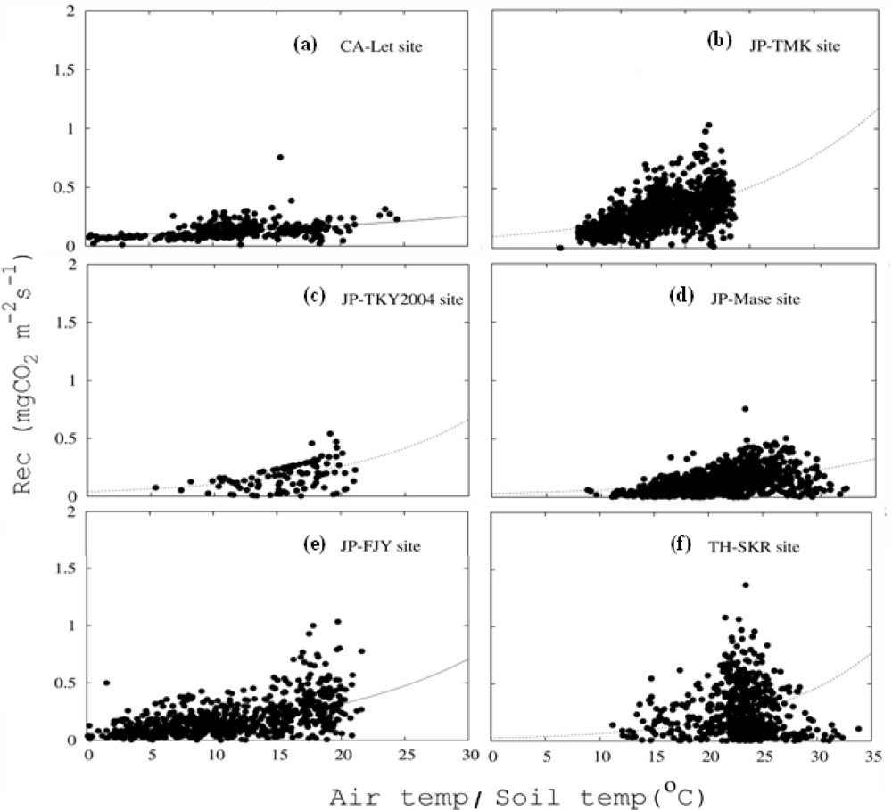
Respiration (Rec) Estimation for the GPP Estimation
Respiration Curve
References
- Saigusa, N.; Yamamoto, S.; Murayama, S.; Kondo, H. Inter-annual variability of carbon budget components in an AsiaFlux forest site estimated by long-term flux measurements. Agric. Forest Meteorol 2005, 134, 4–16. [Google Scholar]
- Saito, M.; Miyata, A.; Nagai, H.; Yamada, T. Seasonal variation of carbon dioxide exchange in rice paddy field in Japan. Agric. Forest Meteorol 2005, 135, 93–109. [Google Scholar]
- Mizoguchi, Y.; Ohtani, Y.; Takanashi, S.; Iwata, H.; Yasuda, Y.; Nakai, Y. Seasonal and interannual variation in net ecosystem production of an evergreen needleleaf forest in Japan. J. Forest Res 2012, 17, 283–295. [Google Scholar]
- Novick, K.A.; Stoy, P.C.; Katul, G.G.; Ellsworth, D.S.; Siqueira, M.B.S.; Juang, J.; Oren, R. Carbon dioxide and water vapor exchange in a warm temperate grassland. Oecologia 2004, 138, 259–274. [Google Scholar]
- Hirata, R.; Hirano, T.; Saigusa, N.; Fujinuma, Y.; Inukai, K.; Kitamori, Y.; Takahashi, Y.; Yamamoto, S. Seasonal and interannual variations in carbon dioxide exchange of a temperate larch forest. Agric. Forest Meteorol 2007, 147, 110–124. [Google Scholar]
- Hirata, R.; Saigusa, N.; Yamamoto, S.; Ohtani, Y.; Ide, R.; Asanuma, J.; Gamo, M.; Hirano, T.; Kondo, H.; Kosugi, Y.; et al. Spatial distribution of carbon balance in forest ecosystems across East Asia. Agric. Forest Meteorol 2008, 148, 761–775. [Google Scholar]


| Band Name | GCOM-C/SGLI Wavelength (nm) | Width | TERRA/MODIS Wavelength (nm) | Width |
|---|---|---|---|---|
| ρblue | 443 | 10 | 469 | 20 |
| ρgreen | 530 | 20 | 555 | 20 |
| ρred | 673.5 | 20 | 655 | 50 |
| ρNIR | 868.5 | 20 | 858.5 | 35 |
| Site Name (data year) | CA-Let 2002, 2003 | JP-TMK 2002, 2003 | JP-TKY 2003, 2004 | JP-Mase 2002, 2003 | JP-FJY 2003, 2004 | US-Dk1 2003 | TH-SKR 2002, 2003 |
|---|---|---|---|---|---|---|---|
| City | Lethbridge | Hokkaido | Takayama | Tsukuba | Yamanashi | Nc | Sakaerat |
| Country | Canada | Japan | Japan | Japan | Japan | US. | Thailand |
| Latitude | 49.709°N | 42.737°N | 36.146°N | 36.054°N | 35.454°N | 35.971°N | 14.492°N |
| Longitude | −112.940°W | 141.519°E | 137.423°E | 140.027°E | 138.762°E | −79.093°W | 101.916°E |
| Plant Functional Types | C3 grass, arctic | NDT | BDT,Temperate | Crop | NET,Temperate | C3 grass | BET,Tropical |
| Dominant species | Short/mixed grass prairie (C3/C4) | Japanese Larch | Deciduous Oak, Birch | Rice | Japanese red pine | Tall fescue,C3 grass and forbs | Dipterocarp |
| Tree age (years) | - | 45 | 50 | - | 90 | 1 | - |
| Elevation (m) | 960 | 140 | 1420 | 13 | 1030 | 163 | 535 |
| Canopy height (m.) | - | 16 | 15–20 | 1.2 | 20 | 0.1–1 | 35 |
| Flux measurement height (m) | 4 | 27 | 25 | 3 | 25.4 | 3 | 45 |
| Annual avg. air temp. (°C) | 5.36 | 6.61 | 7.2 | 12.9 | 10.1 | 15.5 | 24.1 |
| U* threshold (m/s) | 0.2 | 0.3 | 0.5 | 0.1 | 0.12 | 0.2 | 0.2 |
| Reference | Gilmanov et al. 2005 | Hirata et al. 2007 | Muraoka et al. 2005 | Saito et al. 2005 | Mizoguchi et al. 2012 | Novick et al. 2004 | Aguilos et al. 2007 |
| Site name (Year 2003) | Respiration (Rec) Equation | VPD Threshold (kPa) | * Pmax_capacity2000; mg·CO2·m−2·s−1 (Growing Season) | * Initial slope (αslope) |
|---|---|---|---|---|
| CA-Let | Rec = 0.29exp(0.037Tair) | 2 | 0.47 (Apr–Sept) | 0.0029 |
| JP-TMK | Rec = 0.3exp(0.08Tsoil) | 2 | 1.37 (May–Oct) | 0.0016 |
| JP-TKY | Rec = 0.23 × 0.23exp(0.08Tair) | 2 | 0.97 (May–Sept) | 0.0023 |
| JP-Mase | Rec = 0.18exp(0.067Tair) | 2 | 0.96 (May–Aug2) | 0.0017 |
| JP-FJY | Rec= 0.25 × 0.25exp(0.08Tair) | 2 | 1.00 (Apr–Oct) | 0.0014 |
| US-Dk1 | -** | 2 | 0.70 (Apr–Oct) | 0.0035 |
| TH-SKR | Rec = 0.025 × 2.57exp((Tair – 10)/10) | 2 | 1.18 (Apr–Oct, except May2 and June) | 0.0009 |
| Site Name | Plant Functional Types (PFTs) | a | b | R2 |
|---|---|---|---|---|
| CA-Let | C3 grass, arctic | 0.388 | −0.235 | 0.81 |
| JP-TMK | Needleleaf deciduous trees (NDT) | 0.232 | −0.145 | 0.84 |
| JP-TKY | Broadleaf deciduous trees, temperate (BDT, temperate) | 0.169 | −0.355 | 0.67 |
| JP-Mase | Crops (paddy field) | 0.371 | −0.361 | 0.95 |
| JP-FJY | Needleleaf evergreen trees, temperate (NET, temperate) | 0.179 | 0.182 | 0.70 |
Share and Cite
Thanyapraneedkul, J.; Muramatsu, K.; Daigo, M.; Furumi, S.; Soyama, N.; Nasahara, K.N.; Muraoka, H.; Noda, H.M.; Nagai, S.; Maeda, T.; et al. A Vegetation Index to Estimate Terrestrial Gross Primary Production Capacity for the Global Change Observation Mission-Climate (GCOM-C)/Second-Generation Global Imager (SGLI) Satellite Sensor. Remote Sens. 2012, 4, 3689-3720. https://doi.org/10.3390/rs4123689
Thanyapraneedkul J, Muramatsu K, Daigo M, Furumi S, Soyama N, Nasahara KN, Muraoka H, Noda HM, Nagai S, Maeda T, et al. A Vegetation Index to Estimate Terrestrial Gross Primary Production Capacity for the Global Change Observation Mission-Climate (GCOM-C)/Second-Generation Global Imager (SGLI) Satellite Sensor. Remote Sensing. 2012; 4(12):3689-3720. https://doi.org/10.3390/rs4123689
Chicago/Turabian StyleThanyapraneedkul, Juthasinee, Kanako Muramatsu, Motomasa Daigo, Shinobu Furumi, Noriko Soyama, Kenlo Nishida Nasahara, Hiroyuki Muraoka, Hibiki M. Noda, Shin Nagai, Takahisa Maeda, and et al. 2012. "A Vegetation Index to Estimate Terrestrial Gross Primary Production Capacity for the Global Change Observation Mission-Climate (GCOM-C)/Second-Generation Global Imager (SGLI) Satellite Sensor" Remote Sensing 4, no. 12: 3689-3720. https://doi.org/10.3390/rs4123689