The main challenge in ocean color atmospheric correction is the estimation and the removal of the path radiance from the TOA radiance values recorded by the satellite sensor [1]. The path radiance contains both Rayleigh and aerosol scattering components and can contribute about 90% of the TOA radiance [2,3]. In the current version of the NASA ocean color atmospheric correction processing code, spectral aerosol radiance is calculated from a set of 80 aerosol models [4]. This is a more complex modeling system than the previous 12 model set; however the new set of 80 aerosol models reduces the overestimation of AOD and the underestimation of the Angstrom exponent, which was prevalent in the previous set of 12 models [5]. Based on the spectral slope of the aerosol reflectance in the two NIR bands, the two most appropriate aerosol models (from the entire set of 80 models) are retrieved and used for estimation of the aerosol radiance in the visible wavelengths. The question is, are the appropriate models selected?

To answer this question, we compare the satellite-derived _nL_w values to in situ AERONET-OC measurements. We have tested all 80 aerosol models individually with data sets collected from three AERONET-OC sites, Venice, Martha’s Vineyard, and Gulf of Mexico [6–8]. First, we derive spectral _nL_w from the 1 kilometer resolution satellite imagery for both MODIS and SeaWiFS at the locations of AERONET-OC sites, using the aerosol models selected automatically from the standard 80-model atmospheric correction scheme [9]. We compare these satellite values to the in situ_nL_w measurements. We then reprocess the satellite imagery using all 80 aerosol models individually and again compare the retrieved _nL_w values to the in situ measurements. This provides a way to determine the “optimal” aerosol model for each individual point at the AERONET-OC location for each individual satellite scene, where we define the “optimal” model as that aerosol model that yields _nL_w closest to the in situ values. This does not imply that the “optimal” model is the one with the correct aerosol optical properties, but instead is the model that extrapolates the NIR aerosol reflectance in such a way as to absorb the residual error (assuming AERONET-OC, Rayleigh, whitecap, glint, and ozone calculations are all correct, which we know are not the case). We perform this comparison to determine the optimal aerosol model at each individual wavelength; this allows us to assess the “consistency” of the optimal model selection. In other words, is the same “optimal” model selected independently for each wavelength, or do different models at each wavelength yield better results? We also evaluate individual _nL_w retrievals for all 80 aerosol models to show there usually exists several aerosol models, and not just the one “optimal” model or bounding models chosen during standard atmospheric correction, that are capable of producing good spectral _nL_w MODIS to AERONET-OC matchups.

First, we briefly describe ocean color atmospheric correction, the set of aerosol models used, how those models are selected during atmospheric correction, the sensitivity of model selection on relative humidity and size fraction, and possible errors associated with the models. Next, we compare the results using the standard, automatic aerosol model selection to those using the optimal model selection approach described above. In addition, we compare AERONET-measured and satellite-derived AOD values. We perform all these satellite/AERONET-OC analyses for both MODIS and SeaWiFS imagery, at three locations. Finally, we apply noise to the satellite TOA radiance values in the two NIR channels used for atmospheric correction, to determine the effect on aerosol model selection and _nL_w retrievals.

The TOA radiance is defined as follows: (1) L t ( λ ) = L r ( λ ) + L a ( λ ) + L ra ( λ ) + t ( λ ) L wc ( λ ) + T ( λ ) L g ( λ ) + t ( λ ) t 0 ( λ ) cos Θ 0 [ L w ( λ ) ] Nwhere λ is wavelength, L_t(λ) is top-of-atmosphere radiance, L_r(λ) is the radiance due to scattering by the air molecules (Rayleigh scattering) [10–12], L_a(λ) is the radiance due to scattering by aerosols, L_ra(λ) is the multiple interaction term between molecules and aerosols, t(λ) is the diffuse transmittance of the atmosphere from the surface to the sensor, L_wc(λ) is the radiance due to whitecaps on the sea surface [13,14], T(λ) is the direct transmittance from the surface to the sensor, L_g(λ) is the specular reflection of direct sunlight off the sea surface (sun-glitter) [15], t₀(λ) is the diffuse transmittance of the atmosphere from the sun to the surface, θ₀ is the solar-zenith angle, and [L_w(λ)]_N is the normalized water-leaving radiance (_nL_w) due to photons that penetrate the sea surface and are backscattered out of the water [16].

The goal of ocean color atmospheric correction is to retrieve _nL_w(λ) accurately, which is subsequently used to estimate the water bio-optical properties. The main challenge in atmospheric correction is the removal of L_path(λ) from L_t(λ), where L_path(λ) = L_r(λ) + L_a(λ) + L_ra(λ) contributes 80%–100% of the TOA radiance at visible wavelengths [1]. L_r(λ) is determined by the viewing geometry and can be removed from L_path(λ) by using standard radiative transfer methods. The remaining part of L_path(λ), L_a(λ) + L_ra(λ), is estimated from L_t(λ) in the NIR wavelengths. Water is essentially “black” at NIR wavelengths (i.e., totally absorbing), so we can assume that _nL_w is 0 in clear, open-ocean regions at these wavelengths. However, this assumption is not valid in turbid, coastal areas. Several studies have been conducted to analyze aerosol optical properties and aerosol types [17–23]. By assuming that _nL_w is 0 in the NIR, we can calculate L_a(λ) + L_ra(λ). Based on L_a(λ) + L_ra(λ) in the NIR, an estimate is made of L_a(λ) + L_ra(λ) at visible wavelengths. There have been studies conducted that compare and validate the Gordon and Wang 1994 and Ahmad et al. 2010 aerosol models using satellite and AERONET measurements [24,25]. However, no study has yet to be conducted that analyzes the sensitivity and impact of aerosol model selection during atmospheric correction on retrieved spectral _nL_w values, thus affecting down-stream bio-optical properties.

In the most current NASA ocean color processing version, a suite of 80 aerosol models (indexed 0 to 79) are available to compute L_a + L_ra during atmospheric correction. During standard atmospheric processing, there are two aerosol models chosen to bound L_a(λ) + L_ra(λ) in the NIR. The aerosol models are chosen by determining which two aerosol models bound ε(748,869) the tightest, where ε(748,869) is a ratio of AOD, the aerosol single-scattering albedo, and the aerosol scattering phase function, for MODIS (wavelengths 748 and 869) and SeaWiFS (wavelengths 769 and 869) [26]. The ratio is used to select two bounding aerosol models, denoted modmin and modmax. The relative humidity is calculated from climatology before ε(748,869) is calculated, and then ε(748,869) is used to select the size fraction index. Once the two bounding aerosol models are chosen based on ε(748,869), interpolation is performed between the two models and L_a(λ) + L_ra(λ) is retrieved from the aerosol model lookup tables.

The most significant digit in the aerosol model number (ex: the 6 in model 64) denotes relative humidity index. The least significant digit denotes a particle size fraction index. Table 1 lists the different relative humidity and size fraction percentages, along with their corresponding aerosol model index. Regarding the size fractions, a size fraction of 20% denotes 20% fine mode and 80% coarse mode. For example, model 64 corresponds to a relative humidity of 90% and a size fraction of 20%, with 20% being fine mode and 80% being coarse mode.

The primary advantage and reason for separating the aerosol models by relative humidity is to remove the ambiguity that arises in the old Gordon and Wang models where different combinations of size fraction and modal radii (relative humidity) yield the same aerosol reflectance ratio in the NIR (the same epsilon). That ambiguity in model selection leads to sharp transitions in the selected model pairs, which results in scattering-angle dependent discontinuities in the shorter wavelengths. If the relative humidity is known, the model selection can be restricted to just look at variation in size fraction, and thus avoid the ambiguity.

To examine the effect of model selection on retrieved _nL_w, we tested all 80 aerosol models individually for a single clear day, 1 August 2010, in Venice. Instead of using two bounding aerosol models, we used a fixed aerosol model to study the effects of all 80 aerosol models on retrieved _nL_w. This allows visualization of the sensitivity of retrieved _nL_w to aerosol model selection. The _nL_w results at wavelength 488 nm (5 × 5 box mean centered around the AERONET-OC site) are displayed in Figure 1 (other wavelengths have similar patterns).

As stated previously, humidity is calculated from climatology before ε(748,869) is calculated, and then ε(748,869) is used to select the size fraction index. This means that even though there are 80 aerosol models, these are reduced to 10 options because the relative humidity is independent of ε(748,869). For the 1 August 2010 MODIS image, a climatology-based relative humidity of 75% was selected. The bounding aerosol models for individual points within the 5 × 5 box ranged from 31 to 33 (blue box in Figure 1), with a mean modmin value of 32.7 and a mean modmax value of 31.7. The retrieved _nL_w(488) for MODIS and AERONET-OC is 0.98 (blue star in Figure 1) and 1.13 (horizontal blue line in Figure 1), respectively.

To describe the impact of relative humidity and size fraction on retrieved _nL_w values, note the size fraction signified by the bounding aerosol models chosen automatically during standard atmospheric correction. The bounding aerosol model indices ranged from 31 to 33 (size fraction of 80% and 30%, respectively, see Table 1) within the 5 × 5 box. This produced a mean _nL_w(488) value of 0.98. However, if models 35 and 36 (size fraction of 10% and 5%, respectively) had been used, instead of the range of 31 to 33, then the retrieved _nL_w(488) value would be much closer to the AERONET-OC value of 1.13. This model change represents a change in the size fraction, not the relative humidity. We discuss later how a small uncertainty (±2% noise) in TOA L_t values can alter bounding aerosol model selection by 1 or 2 indices, thereby affecting how close the retrieved _nL_w value is to the AERONET-OC value.

The size fraction has a much larger impact than the relative humidity. In Figure 1, the two red lines represent bounding aerosol models that could be chosen to produce good _nL_w matchups, for each relative humidity model index. For example, relative humidities represented by model indices 0–29 (relative humidities of 30% to 70%) would all produce good _nL_w(488) matchups if the size fraction percentages for the bounding aerosol models remained between 20% and 10%. For relative humidities represented by model indices 30–79 (relative humidities of 75% to 95%), good _nL_w(488) matchups would be produced if the size fraction percentages for the bounding aerosol models were between 10% and 5%.

A change in the aerosol model index has a much larger effect on _nL_w retrievals towards the middle size fraction levels (size fraction indices 3–7, denoting 30% to 2%, as seen in Table 1) than in the lowest and highest size fraction levels (size fraction indices 0–2 and 7–9, denoting 95% to 50% and 2% to 0%, respectively). This is evident in Figures 1 and 2. For example in Figure 2(b), for a given relative humidity of 75% (model indices 30–39), models 30–32 show retrieved _nL_w(488) values roughly in the range 0.38 to 0.46, and models 37–39 show retrieved _nL_w(488) values roughly in the range 1.47 to 1.61. However, models 33–36 show retrieved _nL_w(488) values in the range 0.59 to 1.29. Lower relative humidity indices (models 0–29, denoting 30% to 70% relative humidity) tend to have a larger spread of _nL_w values. For example in Figure 2(a), models 0–9 have _nL_w(488) values in the range 1.81 to 3.47. Models 70–79 have a smaller range of nLw values, spanning 2.47 to 3.47. Similar trends are seen in Figure 2(b) and 2(d) but not in Figure 2(c). Selecting inappropriate aerosol models in the middle size fraction indices will result in significant errors in retrieved _nL_w values. Similarly, selecting inappropriate aerosol models in the lower relative humidity indices usually result in larger errors in retrieved _nL_w values.

A variety of aerosol types exist globally and vary based on the season and location. The main aerosol types include dust, sea salt, smoke, and sulfate, where all are the result of natural processes and the latter two may also be the result of anthropogenic activities. The size fraction element used by the set of 80 aerosol models is a rough guide to the type of aerosols present, since each type has an average particle size that is classified as coarse or fine (i.e., dust and sea salt are coarse in comparison to smoke and sulfate). This indicates the size fraction for the chosen model pair should reflect the aerosol types typical for that region. In this paper we compare satellite derived _nL_w radiances and aerosol properties to their corresponding in situ measured values for Martha’s Vineyard, Massachusetts, Venice, Italy, and the northern Gulf of Mexico. In the case of Venice where the predominate aerosol type is anthropogenic pollution (i.e., fine) from Northern Italy, we would expect the fine mode size fraction represented by the set of 80 aerosol models to be greater than 0.5 [27]. In regions with a mixture of fine and coarse aerosol types, such as the Gulf of Mexico and Martha’s Vineyard, the fine mode size fraction is likely to be more variable and influenced by seasonal events such as dust and smoke plumes.

We compare 1 kilometer resolution MODIS _nL_w values to level 1.5 AERONET-OC measured values at these locations: Martha’s Vineyard, Massachusetts (2010, 36 scenes), Venice, Italy (2010, 45 scenes), and northern Gulf of Mexico (2010, 12 scenes). Valid match-ups required no invalid pixels (no atmospheric correction failure or negative _nL_w retrievals), with at least 50% clear pixels in a 5 × 5 box centered on the AERONET-OC location, and AERONET-OC measurements within 3 hours of the satellite overpass (the majority of comparisons are within 1 hour).

First, we downloaded MODIS Collection 5 Level 1 data [28]. We process the MODIS level 1 scenes using the Naval Research Laboratory’s (NRL) Automated Processing System (APS) [29]. APS is a system that ingests and processes AVHRR, SeaWiFS, MODIS, MERIS, OCM, HICO, and VIIRS satellite imagery. It is a complete end-to-end system that includes sensor calibration, atmospheric correction (with near-infrared correction for coastal waters), image de-striping, and bio-optical inversion. All imagery was processed using the NRL APS version 4.2, which features the set of 80 aerosol models. APS version 4.2 is consistent with SeaDAS version 6.3. For our data sets, relative humidity is estimated from climatology. We process numerous areas around the world in real-time, before ancillary data is available. We focus on real-time processing, which is why we used climatological relative humidity values here. Processing data sets using climatology data, rather than ancillary, can sometimes lead to incorrect estimates of relative humidity. If the climatology is close to the ancillary data, then the _nL_w retrievals will not exhibit much change. We have performed comparisons in the past between data sets processed using ancillary and climatology, and we found that spectral _nL_w values usually only changed by 1 to 2 percent. This is due to the size fraction, rather than the relative humidity, having the greatest impact on nLw retrievals. As discussed in the previous section, two bounding aerosol models are selected based on ε(748,869). For the second approach, we process the MODIS scenes using all 80 individual aerosol models. Then, we select a single “optimal” model that yields an _nL_w value closest to the AERONET-OC value.

There is a level of uncertainty in the AERONET-OC measurements. Zibordi et al. concluded that the overall _nL_w uncertainty budget, which is computed as the quadrature sum of the various individual, independent sources of uncertainty, indicates values typically below 5% in the 412–551 nm spectral range and approximately 8% at 667 nm, mostly because of environmental (sea surface) perturbations [30]. Other research has been conducted assessing and improving sky and sun glint methodologies, but the overall approximation of spectral AERONET-OC _nL_w uncertainties remains around 5% [31–33]. Also, AERONET-OC data are produced at wavelengths which are slightly different from site to site, as well as slightly different from the wavelengths used by MODIS and SeaWiFS. Zibordi et al. have assessed the uncertainty between these differences and applied a band-shift correction scheme based on regional bio-optical algorithms [34]. For this work, we have not applied the band-shift correction.

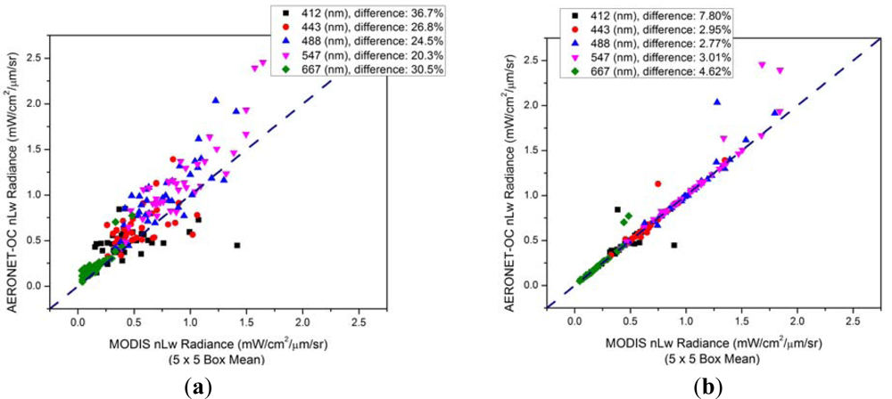
For the analysis of Martha’s Vineyard, 2010, we determine the optimal aerosol model separately for each visible wavelength. Figure 3 displays the _nL_w matchups for satellite standard processing vs. in situ, as well as satellite processing with optimal aerosol model selection vs. in situ. The relative percent differences (RPD) (calculated as the absolute value of (((MODIS − AERONET-OC)/AERONET-OC) × 100) are greatly reduced with the optimal model selection, indicating that the automatic model selection procedure may not be selecting the “optimal” model, in terms of achieving the closest matchups between the satellite-estimated _nL_w values and the AERONET-OC-measured values.

Due to potential uncertainty in pixel geo-location or adjacency effects due to the Martha’s Vineyard AERONET-OC site being less than two nautical miles from the coast, we ran a comparison between a 5 × 5 box mean, center pixel only, and the AERONET-OC value at the 412 nm wavelength. As seen in Figure 3, the RPD for all scenes in the data set between the MODIS box mean and the AERONET-OC value is 36.7%. The RPD between the MODIS center pixel (closest to the AERONET-OC station) and AERONET-OC is actually slightly worse at 39.6%. The MODIS box mean compared to the MODIS center pixel has a RPD of 15.8%. We plotted the 1:1 relationship between the MODIS box mean and the MODIS center pixel, and there was no noticeable bias, so we used a 5 × 5 box at the Martha’s Vineyard location to remain consistent with the Venice and Gulf of Mexico analyses.

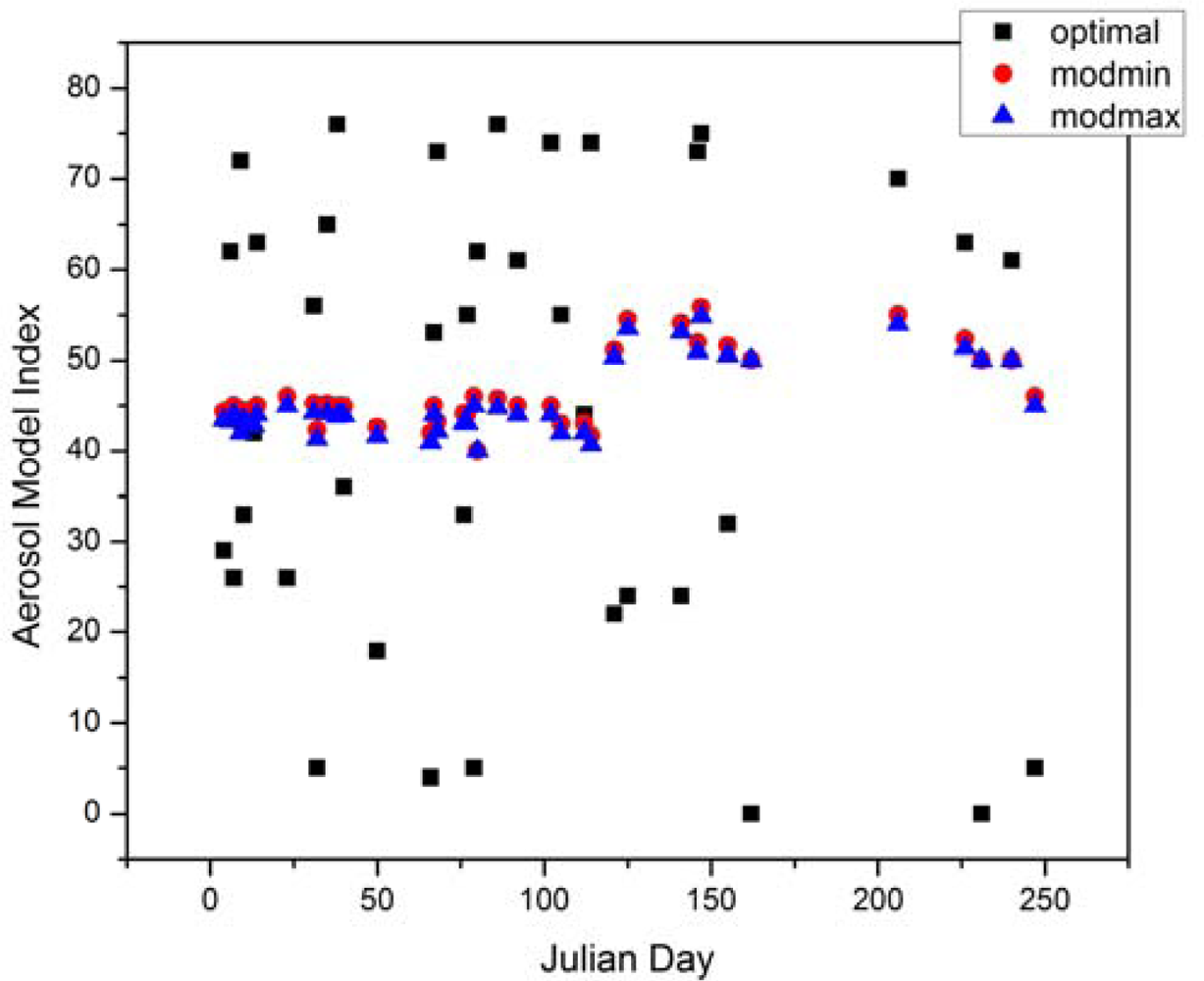
Using the same data set, in Figure 4 we show the optimal aerosol model selected for computing _nL_w(412), as well as the bounding aerosol models selected during standard, automated atmospheric processing. Figure 4 shows a wide spread of optimal aerosol model selections through 2010 for Martha’s Vineyard (non-integer aerosol model index values in this figure are a result of averaging the index values within a 5 × 5 box centered around the AERONET-OC site). This is due to relative humidity index varying throughout the optimal models chosen for this data set. The optimal model for a particular sample in the data set is based on how close the satellite-retrieved _nL_w is to the AERONET-OC measured value. The optimal model is chosen out of the complete set of 80 aerosol models. However, as stated previously, during standard, automated atmospheric correction, relative humidity is calculated before ε(748,869), and only size fractions for that relative humidity index are available as possible bounding aerosol models, thus reducing the set of 80 possible aerosol models down to 10. The optimal models do not indicate that the relative humidity used in the standard, automated atmospheric correction is incorrect; it simply indicates a wide range of relative humidity values that can give approximately “correct” retrievals (with “correct” indicating a value close to the AERONET-measured value). It also indicates more than one model is capable of producing an _nL_w value that closely matches the AERONET-OC value. For example, in Figure 1 we can see that models 35, 45, 55, 65, and 75 all yield similar _nL_w values (∼1.12).

Bounding aerosol models selected during standard, automated atmospheric correction are the two models that bound ε(748,869) the tightest. The model with the larger index (modmin) is usually one index higher than the model with the smaller index (modmax). However, there are four points in Figure 4 where modmin and modmax are the same (days 80, 162, 231, and 240). When ε(748,869) does not fall between two bounding aerosol models in the look-up table, modmin is the same as modmax. It indicates ε(748,869) is either lower than the ε(748,869) in the look-up tables for the lowest available bounding aerosol model or higher than the ε(748,869) in the look-up tables for the highest available bounding aerosol model (for a given relative humidity). In this case, it almost always leads to a poor estimate of the aerosol composition, which in turn results in an erroneous estimate of _nL_w values. From our data sets, we observed modmax = modmin for less than 2% of all valid pixels. When it did occur, it was usually along or near the coastline; however, there were instances when it occured toward the open ocean. This was usually the result of light to moderate haze, which is not thick enough to be flagged as clouds; however, it can occur when no haze or clouds are evident. 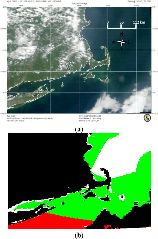Figure 5 displays a scene where clear, cloud, and hazy pixels all have equal modmin and modmax values.

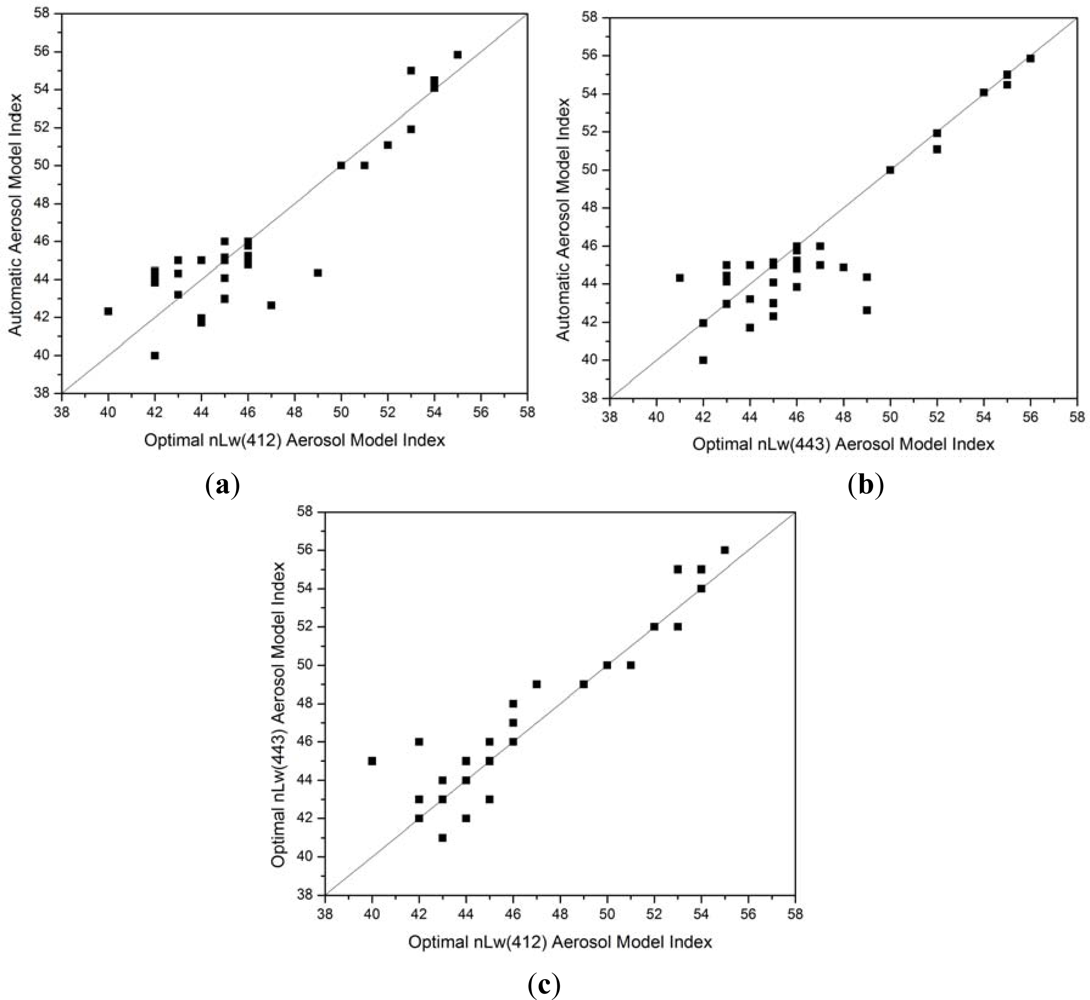
To assess the effect of size fraction on model selection, independent of relative humidity, we compare aerosol models selected during standard, automated atmospheric correction and optimal aerosol models selected using the same relative humidity. This narrows the set of optimal aerosol model possibilities for any given point from 80 to 10 models, thus optimizing only the size fraction, not the relative humidity. Because a 5 × 5 box mean of aerosol indices is taken from each automated value, we consider an optimal model index (all model indices inside the 5 × 5 box are the same due to the same aerosol model being applied at each pixel, therefore no floating point value may occur) to match the automated model index when the optimal model is within ±0.5 of the automated model index.

As seen in Figure 6, most of the optimal models do not match the models selected during standard, automated atmospheric correction. Thus, even within a given relative humidity, the automated model selection is not optimal. Out of the 36 points in the Martha’s Vineyard 2010 dataset, the optimal model selected for _nL_w(412) matches the automatic model only 9 times (25%, Figure 6(a)), and the optimal model selected for _nL_w(443) matches the automatic model 14 times (38.9%, Figure 6(b)). In Figure 6(c), we compare the optimal model selected for _nL_w(412) to the optimal model selected for _nL_w(443). These values match 15 out of 36 times (41.7%), indicating that a single aerosol model may not be optimal for all wavelengths (i.e., the available aerosol models are not adequate to fully represent the spectral variability).

Using the same data set, Figure 7 shows a comparison between the AERONET-OC and MODIS _nL_w(λ) values determined using optimal aerosol models selected from the set of 10 possible aerosol models (representing size fraction) after the relative humidity has already been determined from climatology. Table 2 gives a summary of the RPD between MODIS and AERONET-OC _nL_w values, for automatic aerosol model selection and optimal aerosol model selection using the full set of 80 aerosol models, as well as the confined set of 10 aerosol models for the current relative humidity. We find that when we optimize only the size fraction, we can improve _nL_w matchups, although they are not as good as when we also optimize the relative humidity (Figure 3(b)).

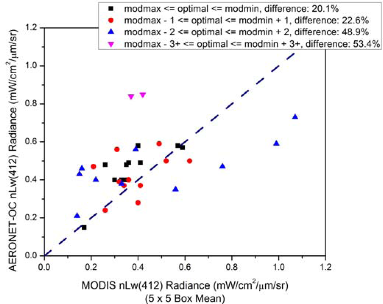
In Figure 8, using the same data set as in Figures 3–7, we perform another sensitivity analysis to examine the effect of aerosol size fraction on _nL_w retrievals. We examine differences between AERONET-OC and MODIS _nL_w(412) values for 4 cases: when the automatically-retrieved aerosol size fraction matches the size fraction of the optimal model, when the size fraction is within 1 index number of the optimal size fraction, when it is within 2, and when it is within 3, where the optimal model in each case is the optimal aerosol model selection from the set of 10 possible aerosol models available after the relative humidity has been determined from climatology. For Figure 8, we remove the data points in the first group where the bounding aerosol models have the same size fraction (modmin and modmax are both equal to zero, days 162 and 231 with observed RPD of 38.4% and 217%, respectively). These are treated as bad data points, for reasons previously discussed. This drops the data set from 36 to 34 points. There are 11 data points in the first group, 11 in the second group, 10 in the third group, and 2 in the fourth group. Points that fall in the first group indicate that the size fraction is likely to have been correctly selected during standard, automated atmospheric correction. This means that standard processing accurately selected bounding aerosol models for only 11 of the 36 points. When the automatically-retrieved size fraction matches the size fraction of the optimal model, the average RPD between the MODIS-retrieved _nL_w and the AERONET-OC nLw is 20.1%; RPDs increase for the other three cases as shown in Figure 8. We are only assessing the effect of size fraction here, not relative humidity. These results indicate that even a relatively small RPD in the size fraction retrieval (off by a single index value) can lead to significant RPDs in retrieved nLw.

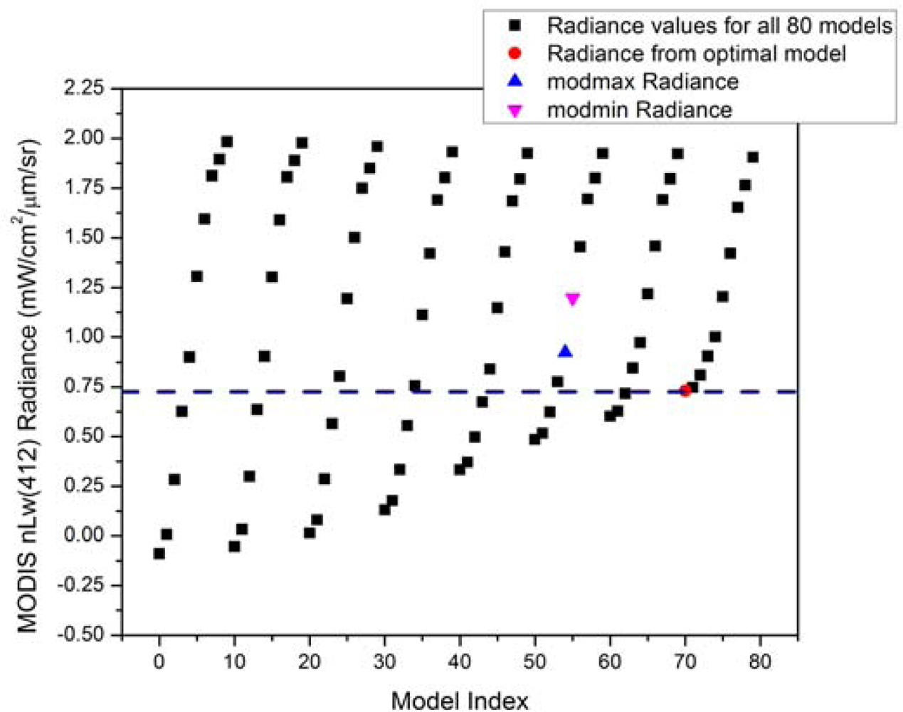
To further examine the impact of aerosol model selection on _nL_w retrieval, we apply all 80 models to the MODIS image covering Martha’s Vineyard on 25 July 2010, and we compare the retrieved values to the in situ AERONET-OC measurement at that location (Figure 9). During standard, automated processing, the mean _nL_w(412) value within a 5 × 5 box surrounding the AERONET-OC site is 1.07344, and the two bounding aerosol models selected are 54 and 55. The optimal model that yields a retrieved _nL_w(412) closest to the in situ value (0.7254 mW/cm²/μm/sr) is model 70 (retrieved _nL_w(412) = 0.7298 mW/cm²/μm/sr). Standard processing indicates a retrieved relative humidity of 85% (since the model index is in the 50s, see Table 1), and the optimal model indicates a retrieved relative humidity of 95% (since the model index is in the 70s). The significant difference in the bounding models selected during standard processing and the optimal model is the size fraction. The modmax bounding model (model 54) yields an _nL_w(412) value of 0.9222; the modmin bounding model (model 55) yields a value of 1.1973. The retrieved _nL_w(412), weighted by ε(748,869), is 1.07344. Despite an optimal aerosol model selection of 70 in this example, there are multiple aerosol modmin/modmax models that can yield an _nL_w value that closely matches the AERONET-OC’s measurement, for example any two models that bound the dashed line in Figure 9. If we stay in the standard processing relative humidity (85%), models 52 and 53 could be used to produce a better _nL_w value. In this example, ε(748,869) is computed from the image and non-optimal bounding aerosol models are selected. If models 52 and 53 had been selected, the retrieved _nL_w value would more closely match the in situ value. This example illustrates that incorrect selection of bounding aerosol models can lead to errors of 10% or greater between MODIS-retrieved _nL_w values and AERONET-OC values.

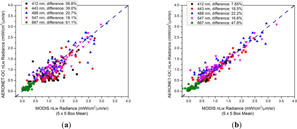
For the Venice 2010 data set, we determine the optimal aerosol model based on _nL_w(412) for 53 individual points (each point is a separate MODIS satellite image; each individual image represents a single day) at the AERONET-OC location. We then use that optimal model to calculate _nL_w at the remaining wavelengths, rather than calculating the optimal model for each wavelength separately, as we did with the Martha’s Vineyard evaluation (Figures 3–9). We chose to use the optimal model at _nL_w(412) as a test case because _nL_w(412) generally has the highest RPD. Future research could involve better estimates of an “optimal” model by performing a spectral mean matchup analysis. Even when the optimal model derived from _nL_w(412) is applied to the other visible wavelengths, RPDs are still significantly reduced for most wavelengths (Figure 10). For example, RPDs are reduced from 39.0% at 443 nm using the standard processing to 18.5% using the 412 nm optimal model.

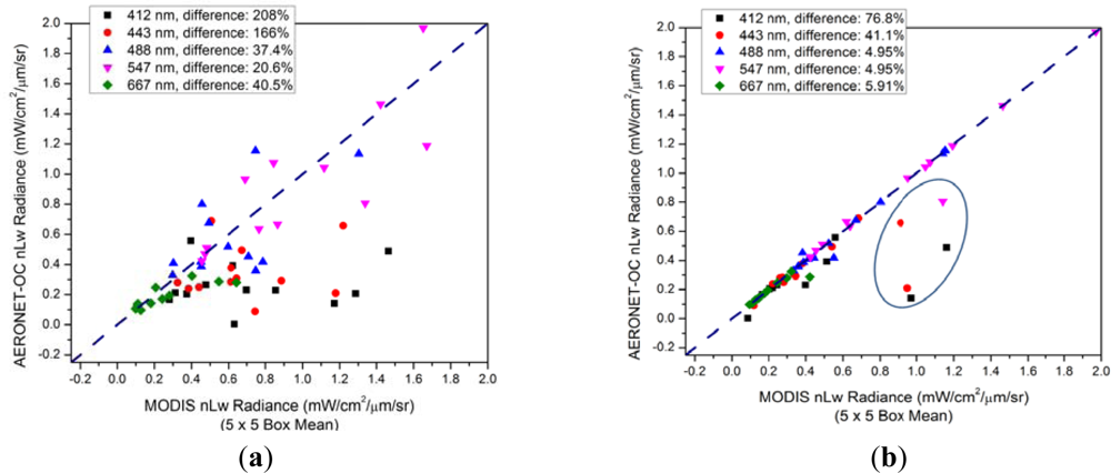
Figure 11 shows the results from a similar analysis for the Gulf of Mexico AERONET-OC site in 2010. However, this comparison does not have as many valid match-up points as the Martha’s Vineyard or Venice comparisons. This is due to a large number of cloud-contaminated MODIS pixels at the site during the year, as well as fewer AERONET-OC values because the station was unavailable for a few months while the instrument underwent calibration. For two of the MODIS images, there are no good aerosol models available that are capable of producing a matchup close to the corresponding in situ value. There are five data points (circled) in Figure 11 that correspond to these two MODIS images (two _nL_w(412) values, two _nL_w(443) values, and one _nL_w(547) value). Three of these five values (one _nL_w(412) value, one _nL_w(443) value, and one _nL_w(488) value) correspond to day 176. For day 176, both modmin and modmax are equal to forty, meaning these bounding aerosol models are likely incapable of producing good _nL_w retrievals, as discussed previously. In this case, none of these aerosol models will yield an _nL_w close to the AERONET-OC value on day 176. Although sporadic clouds and haze are visible in this scene, enough pixels in the 5 × 5 box met the criteria to be considered a valid match-up. However, when none of the aerosol models yield an _nL_w value close to the AERONET-OC value, it might indicate haze contamination in the imagery, even though the pixels are not flagged as clouds.

So far we have compared _nL_w retrievals from MODIS and AERONET-OC. We have analyzed the impact of aerosol model selection on _nL_w retrievals during standard atmospheric correction. We compared the automatically selected bounding models to the optimal models for multiple clear images at three AERONET-OC locations. Now we compare SeaWiFS and MODIS aerosol model selection and _nL_w retrievals using standard, automated atmospheric correction for nearly coincident images (collected within three hours of each other) covering the Venice AERONET-OC site in 2010. Because of the short time difference between the images collected by the two sensors, we expect that the aerosols are fairly similar, so we would also expect, in general, similar aerosol model selection. However, it is not unreasonable to expect some differences between the SeaWiFS and MODIS aerosol models selected, because differences in sensor calibration, viewing geometry, wavelengths (sensor response functions), signal:noise in each channel, and measurement error can lead to differences in the L_t measurements for the two sensors. In addition, for MODIS, ε is calculated using the 748 nm and 869 nm bands, whereas for SeaWiFS, the 769 nm and 869 nm bands are used.

We compare 15 clear MODIS and SeaWiFS images collected within three hours of each other, and with AOD(865) <0.2 for both sensors. Table 3 shows the time difference between the corresponding MODIS and SeaWiFS images, as well as the mean modmin bounding aerosol models selected (modmin and modmax) for the 5 × 5 box centered on the AERONET-OC site. The modmin aerosol models are those selected for the original sensor-measured L_t(748) radiances, as well as those selected with ±2% noise applied to L_t(748), to assess the effect of L_t(748) uncertainty on aerosol model selection. 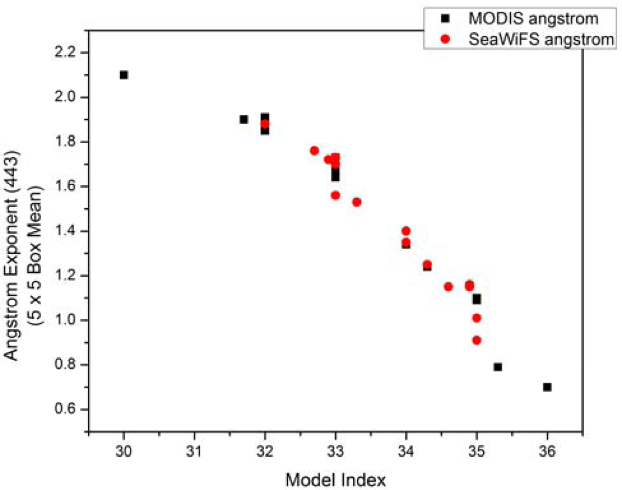For the original sensor-measured L_t(748) radiances, we have included the angstrom coefficient, α, for both the MODIS and SeaWiFS data sets. For the calculation of the angstrom coefficient, we used wavelengths 443 and 869 for MODIS and wavelengths 443 and 865 for SeaWiFS. Figure 12 demonstrates the relationship between model index and α(443).

For the MODIS/SeaWiFS comparison with no noise added, in 9 of the 15 cases, box mean modmin aerosol model indices differed by more than one for the coincident MODIS and SeaWiFS images. However, even for the cases where the same aerosol models were selected, the calculated _nL_w values for MODIS and SeaWiFS could differ (as well as the subsequent bio-optical properties), due to the different L_t(λ) values recorded by the two sensors (for the reasons mentioned above).

Uncertainty in the L_t measurements can lead to uncertainty in the calculation of ε(748/769,869), which in turn can lead to selection of incorrect bounding aerosol models. We demonstrate this effect by performing a sensitivity test in which we add noise (±2%) to the L_t(748) values for the 15 MODIS and SeaWiFS images in Table 3. Vicarious gain coefficients that are applied to the MODIS Lt values during calibration are in the range of 1–3%, with the current gain applied to Lt(748) equaling 0.9855 [35]. Also, 2% noise seems to bind observed variability in image climatology and AERONET-OC data [36]. In most cases, increasing or decreasing L_t(748) by 2% or less impacts ε calculation and model selection.

Just a one percent change in L_t(748) is usually enough to alter the bounding aerosol model index by one for each image (Table 3). A two percent change in L_t(748) sometimes alters the index by two. Even if the bounding models do not change, a change in ε(748/769,869) impacts _nL_w retrievals since ε(748/769,869) is used to interpolate the radiances between the bounding aerosol models. This can have a significant impact, especially in the middle size fractions, where large radiance differences are observed, even for consecutive model index numbers (see Figure 2).

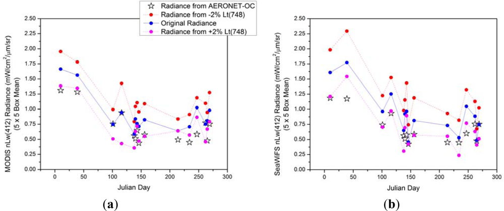
The impact of a ±2% change in L_t(748) for MODIS and L_t(765) for SeaWiFS on the _nL_w radiance retrievals at the Venice AERONET-OC site in 2010 is shown in Figures 13 and 14 for two visible wavelengths, along with the corresponding AERONET-OC _nL_w measurements (similar patterns were observed for the other visible wavelengths). These figures show the temporal variability in the AERONET-OC-measured values and the satellite-derived values over a one-year period, and demonstrate the magnitude of change in the satellite _nL_w values that would result from a ±2% change in the TOA satellite radiance measurements at a single NIR wavelength (such as that due to sensor calibration drift). Note that in most cases, the original, automatically derived satellite _nL_w is quite different from the AERONET-OC measurement and often fall outside of the ±2% noise envelope.

Also note that the AERONET-OC _nL_w values differ slightly between the MODIS and SeaWiFS figures because the AERONET-OC _nL_w values selected were those closest in time for each sensor. By varying L_t(748) in MODIS and L_t(769) in SeaWiFS, we are able to get a better understanding of just how much a one or two percent uncertainty in the NIR Lt measurements can affect the _nL_w retrievals at the visible wavelengths.

In Figures 13 and 14, the points that fall outside of the ±2% noise envelope can help elucidate possible sensor issues or seasonal trends in the data. For instance, in Figure 11, MODIS consistently overestimates the AERONET-OC _nL_w(412) measurements. Only 5 of 15 AERONET-OC points fall within the ±2% aerosol bounds. MODIS overestimates _nL_w(412) for all 10 point comparisons that do not fall within these bounds. Also, over-estimation is more prevalent during the winter months, possibly indicating atmospheric conditions (haze or aerosols) during that season that are not properly corrected for during the atmospheric correction process. SeaWiFS has similar issues but has better AERONET-OC matchups in the later months of the year. Still, only 7 of 15 AERONET-OC points fall within the ±2% aerosol bounds for SeaWiFS.

MODIS _nL_w(547) has better matchups than SeaWiFS nLw(555), despite AERONET-OC using the same wavelength as SeaWiFS (555) for the comparison (Figure 14). 13 of the 15 AERONET-OC points fall within the ±2% aerosol bounds for MODIS, and 7 of 15 AERONET-OC points fall within the ±2% aerosol bounds for SeaWiFS. Even where the AERONET-OC points fall outside of the bounds for MODIS, they are still usually very close; however, both MODIS and SeaWiFS tend to under-estimate the AERONET-OC values. For MODIS, 1 point that does not fall within the ±2% aerosol bounds is underestimated, and for SeaWiFS 5 of the 8 points that do not fall within the ±2% aerosol bounds are underestimated. Both MODIS and SeaWiFS exhibit a seasonal trend to underestimating the radiance values during the winter months.

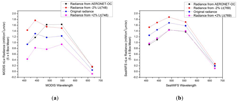
Figure 15 shows the spectral variability related to the addition of noise in a single NIR channel (748 for MODIS, 769 for SeaWiFS) at the level of ±2%, for 16 April 2010, Venice. In the MODIS image (Figure 15(a)), the original MODIS radiance (no noise added) produces a good matchup with the radiance from AERONET-OC, in the 412 and 443 wavelengths. However, the − 2% noise applied to L_t(748) produces good matchups in the remaining visible wavelengths (488, 547, and 667). In the SeaWiFS image, the +2% noise applied to L_t(769) produces good matchups in all visible wavelengths except for 670, where the original radiance produces a good matchup.

Just a 1%–2% uncertainty in MODIS L_t(748) or SeaWiFS L_t(765) is usually enough to change the bounding aerosol models selected during atmospheric correction, which in turn has a significant impact on the _nL_w retrievals in the visible wavelengths. During standard atmospheric processing, bounding aerosol models are selected from the L_t NIR and then used to correct the visible wavelengths. The trends highlighted above (MODIS and SeaWiFS over-estimating in the 412 wavelength and under-estimating in the 547, MODIS, and 555, SeaWiFS, wavelengths) could indicate that incorrect aerosol models are often selected, or that additional, more appropriate aerosol models are required. Also, continuous vicarious calibration of ocean color sensors is required to ensure accurate L_t retrievals which will subsequently yield accurate _nL_w retrievals.

We now compare the size fraction represented by the automatically-selected bounding aerosol models for MODIS and SeaWiFS to size fraction estimates from the AERONET station in Venice. Total AOD, coarse AOD, and fine AOD at 500 nm are recorded at the AERONET sites. We compare this size fraction data from the SDA Level 1.5 (cloud screened) AERONET processing to the size fraction represented by the bounding aerosol models (calculated from ε) determined during standard, automated atmospheric processing for both MODIS and SeaWiFS imagery (see Table 1 for model/size fraction descriptions).

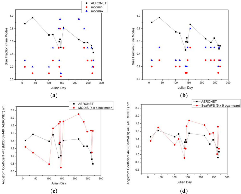
Figure 16 shows the size fraction represented by the bounding aerosol models (modmin and modmax) for both MODIS and SeaWiFS compared to the size fraction estimated by AERONET. The aerosol models use fixed modes, based on averages observed in a subset of AERONET retrievals, but the individual AERONET retrievals used in these matchups are for bimodal distribution based on model inversion that can vary significantly in modal radii. Because the modal radii and width are not identical for this comparison, Figure 16 also shows α(443) for MODIS and SeaWiFS compared to α(440) for AERONET.

In Figure 16 the MODIS and SeaWiFS size fraction retrievals from the aerosol models are usually lower than those of AERONET. To improve satellite/in situ radiance matchups, one option might be to select the satellite aerosol model based on the AERONET size fraction retrieval. However, when the size fraction increases, the aerosol model index decreases (see Table 1), which decreases the _nL_w retrievals as well (see Figures 1 and 2). Thus, the _nL_w retrievals would all decrease if we force the size fraction from MODIS and SeaWiFS to match those of AERONET. This may improve _nL_w retrievals in the 412 and 443 wavelengths for Venice 2010 (since MODIS and SeaWiFS have a tendency to over-estimate _nL_w for these wavelengths), but retrievals for the remaining visible wavelengths would be worse on average, compared to AERONET.

For example, day 39 for MODIS uses bounding aerosol models of 35 and 34. Model 34 represents a size fraction of 20%, and model 35 a size fraction of 10%. AERONET reported a size fraction of 97.4% for that day. Model 30, representing a size fraction of 95%, is the model with a size fraction closest to the observed AERONET measurement. If AERONET is a good measure of size fraction, then the automatically selected models (34 and 35) are not close to the model suggested by the AERONET measurement (30). Forcing MODIS to use model 30 would significantly decrease the _nL_w retrievals, likely resulting in severe under-estimation of _nL_w for most, if not all, visible wavelengths (as described above).

We also assess the impact of size fraction on _nL_w retrievals. Since there is poor agreement between MODIS and AERONET size fraction on day 39, one might expect poor _nL_w matchups as well. However, the values agree closely on this day (Table 4). The MODIS size fraction modmin = 10%, modmax = 20%, and the AERONET size fraction = 97.37%, yet the _nL_w matchup RPDs at all wavelengths are 12% or less, with an average _nL_w RPD across all wavelengths of 6.1%. This demonstrates that even if the aerosol size fractions do not agree between MODIS and AERONET, there can still be very good _nL_w matchups. On day 234, a day when the AERONET size fraction falls in between the size fractions represented by the MODIS bounding aerosol models, suggesting that there might be good agreement between the measured and retrieved _nL_w values, we in fact see poor agreement. On day 234, the MODIS size fraction modmin = 50%, modmax = 80%, and the AERONET size fraction = 58.2%, with an average _nL_w RPD across all wavelengths of 36.6%. Similar trends exist when comparing individual satellite to AERONET angstrom coefficient matchups to their respective _nL_w matchups. There exists a seasonal trend for the angstrom coefficient plots seen in Figure 16(c,d). Both MODIS and SeaWiFS underestimate α(443) in the winter months and overestimate α(443) the remainder of the year. However, the SeaWiFS α(443) matchups, as well as _nL_w matchups, are overall significantly better than the MODIS matchups, The α(443) RPD for MODIS and SeaWiFS comparisons to AERONET are 40.2% and 19.9%, respectively. The spectral _nL_w RPD for MODIS and SeaWiFS comparisons to AERONET are 39.8% and 23.9%, respectively, thus possibly indicating that the better α(443) RPD observed for SeaWiFS led to better spectral _nL_w RPD.

A comparison between MODIS- and SeaWiFS-derived size fraction values is shown in Figure 17. Of the 15 comparison points, 2 have coincident values (thus only 13 points in Figure 15). Out of the 15 comparison points for the Venice 2010 data set, only four used the same bounding aerosol models (days 10, 156, 247, and 269). The _nL_w retrievals for these four points are shown in Table 5.

Next, we compare AOD retrievals from MODIS and SeaWiFS to the AERONET measured values at the Venice location for 2010 (Figure 18), to assess whether good/poor AOD matchups lead to good/poor _nL_w matchups (Figure 19). In general, there is good agreement between the satellite and AERONET AOD values.

Day 101, however, has a poor MODIS vs. AERONET AOD matchup (346%, Figures 18 and 19, red circled point), but this does not lead to poor _nL_w matchups. Day 101 has RPDs of 6.8% for _nL_w(412), 7.0% for _nL_w(443), 2.9% for _nL_w(488), 6.4% for _nL_w(547), and 22.3% for _nL_w(667). Day 146 (Figures 18 and 19, blue circled point) also has a poor AOD matchup (180%) but good _nL_w matchups in the 488 and 547 bands and poor matchups in the remaining bands; 98.4% RPD for _nL_w(412), 39.3% for _nL_w(443), 5.6% for _nL_w(488), 9.3% for _nL_w(547), and 29.2% for _nL_w(667). The same pattern is apparent for the SeaWiFS vs. AERONET comparison. Days 138 and 156 (Figures 18 and 19 green and purple circled points, respectively) have poor AOD matchups (115% and 47%, respectively), yet _nL_w matchups for day 138 are very good, while day 156 is similar to day 146 in the MODIS vs. AERONET image. Day 138 has RPDs of 15.5% for _nL_w(412), 18.4% for −_nL_w(443), 0.8% for _nL_w(490), 8.5% for _nL_w(555), and 21.4% for _nL_w(670). Day 156 has RPDs of 39.3% for _nL_w(412), 33.0% for _nL_w(443), 9.2% for _nL_w(490), 4.4% for _nL_w(555), and 18.0% for _nL_w(670).

Day 101 in Figure 19(a) (MODIS), and day 138 in Figure 19(b) (SeaWiFS) are days where the satellite/AERONET AOD differences were the largest. However, _nL_w errors for these days are very small. A good/poor _nL_w matchup does not necessarily correspond to a good/poor AOD matchup, even though AOD is used in the computation of ε(748/769,869) as shown in equation 5 in [5].

There is ambiguity when comparing model-inferred aerosol optical properties, such as AOD and the angstrom coefficient, to AERONET retrieved optical properties. The Gordon and Wang/Ahmad et al. atmospheric correction approach uses measured NIR aerosol reflectance to select the most appropriate model. Using the models and the reflectance, aerosol optical properties such as AOD and the angstrom coefficient can be inferred, but it is the reflectance that is measured (in the NIR). The fact that the inferred aerosol optical properties do not match AERONET retrieved optical properties does not indicate that the reflectance is wrong, since many combinations of aerosol optical properties can yield the same reflectance. This may be the reason why poor AOD matchups observed in Figures 18 and 19 can still lead to good _nL_w matchups.

In this paper, we have compared satellite normalized water-leaving radiance (_nL_w) retrievals to in situ AERONET-OC measurements for Martha’s Vineyard, Venice, and the Gulf of Mexico. During standard, automated atmospheric correction, selection of inappropriate or erroneous bounding aerosol models can dominate the errors in the satellite estimation of _nL_w. Errors in _nL_w will in turn affect downstream bio-optical properties. When bounding aerosol models are incorrectly chosen during atmospheric correction, it is the size fraction, rather than the relative humidity, that has the most impact on retrieved _nL_w values. If bounding aerosol models are incorrectly selected, there is usually another set of models within the same relative humidity index that are capable of producing accurate _nL_w retrievals.

We also directly compared _nL_w retrievals from MODIS and SeaWiFS imagery, as well as AERONET-OC stations. MODIS and SeaWiFS imagery of the same region of interest, taken within three hours of each other, usually have different bounding aerosol models chosen during standard atmospheric correction. We demonstrated that as little as 1% or less uncertainty (noise) in the NIR L_t radiances can lead to the selection of a different pair of bounding aerosol models, thus changing _nL_w retrievals.

We found that there is a large discrepancy between aerosol size fraction values retrieved by MODIS, SeaWiFS, and AERONET. However, a good size fraction matchup does not necessarily translate to a good _nL_w matchup; similarly, poor size fraction matchups do not necessarily translate to poor _nL_w matchups.

Finally, we compared AOD retrievals from MODIS, SeaWiFS, and AERONET. Even though AOD is a fundamental parameter associated with the aerosol models determined by the satellite ε(748/769,869) value, a good satellite matchup with AERONET does not ensure a good _nL_w matchup. This may be a result of the ambiguity when comparing model-inferred aerosol optical properties, such as AOD and the angstrom coefficient, to AERONET retrieved optical properties.

All downloaded level 1 MODIS data is from Collection 5. Analysis with data Collection 6 (which are derived using new calibration coefficients, particularly for the blue bands) may decrease some of the MODIS to AERONET-OC _nL_w differences.