Article

Measurement of Surface Displacement and Deformation of Mass Movements Using Least Squares Matching of Repeat High Resolution Satellite and Aerial Images

Department of Geosciences, University of Oslo, P.O. Box 1047, N-0316 Oslo, Norway
*
Author to whom correspondence should be addressed.
Remote Sens. 2012, 4(1), 43-67; https://doi.org/10.3390/rs4010043
Submission received: 10 November 2011 / Revised: 19 December 2011 / Accepted: 21 December 2011 / Published: 4 January 2012

Abstract

:
Displacement and deformation are fundamental measures of Earth surface mass movements such as glacier flow, rockglacier creep and rockslides. Ground-based methods of monitoring such mass movements can be costly, time consuming and limited in spatial and temporal coverage. Remote sensing techniques, here matching of repeat optical images, are increasingly used to obtain displacement and deformation fields. Strain rates are usually computed in a post-processing step based on the gradients of the measured velocity field. This study explores the potential of automatically and directly computing velocity, rotation and strain rates on Earth surface mass movements simultaneously from the matching positions and the parameters of the geometric transformation models using the least squares matching (LSM) approach. The procedures are exemplified using bi-temporal high resolution satellite and aerial images of glacier flow, rockglacier creep and land sliding. The results show that LSM matches the images and computes longitudinal strain rates, transverse strain rates and shear strain rates reliably with mean absolute deviations in the order of 10−4 (one level of significance below the measured values) as evaluated on stable grounds. The LSM also improves the accuracy of displacement estimation of the pixel-precision normalized cross-correlation by over 90% under ideal (simulated) circumstances and by about 25% for real multi-temporal images of mass movements.

1. Introduction

Remote sensing is highly suited for slope monitoring in inaccessible areas such as high mountains and cold regions where mass movement processes such as glacier flow, permafrost creep and rock sliding are common. Repeat optical image matching is used to compute displacements on slope movements within the temporal baseline of the images’ acquisitions [16]. The most commonly used group of image matching methods, for that purpose, are area-based methods, where intensities of image patches (hereafter referred to as templates), usually of square shape and pre-defined size, are matched using a chosen similarity measure. The template within the search image that maximizes similarity or minimizes dissimilarity (depending on the statistic) with the reference template is considered the most likely match [7]. The Euclidean distance between the positions of the reference and the matching templates quantifies displacement, specifically the horizontal displacement component if orthorectified image data are used. The displacement gradient between neighboring templates defines the strain [8,9]. Although there is a range of possible similarity measures [7,10], the normalized cross-correlation (NCC) is the most widely used due to the normalization that makes it insensitive to differences in brightness and contrast [11].
The NCC, and other similarity measures, is subject to a number of shortcomings: (1) The NCC is only reliable in cases where the template is not significantly deformed, but only shifted in position. (2) The precision with which the matching position is located is limited to the pixel size unless sub-pixel precision procedures [12] are applied. (3) Radiometric differences are not accounted for except normalizing (i.e., a radiometric offset and gain). Thus, the images are matched with a lower precision and accuracy than theoretically possible. In response to these shortcomings least squares matching (LSM) was designed [13]. Instead of assuming exact shape and size of the matching templates, LSM models both geometric and radiometric distortions. The model parameters are determined iteratively using least squares adjustment. The LSM has no limitation of precision as the location of the matches can theoretically be determined at any sub-pixel precision.
Matching of orthorectified and co-registered bi/multi-temporal images of the Earth surface can be thought of as looking to the changing object from a fixed camera multiple times with small (or absent) spatial baselines and dominant temporal baselines. The spatial transformation models are in this case used to model the distortion of the mass, not the perspective one as done in multi-angular parallax matching [14]. The models can thus be used to directly compute intra-template deformation parameters such as normal strain rates, shear strain rates and rotation. The computation of displacement using LSM by itself leads to improved precision of the computed strain even when strain rates are computed in a separate step, after the matching, from displacement gradients as is conventional practice. The fact that the LSM is able to model the template’s geometric deformation has also the advantage that larger template sizes with higher signal-to-noise ratios (SNR) can be used for the matching as the intra-template deformation, which normally limits the template size, is accounted for.
There is limited application of this powerful image matching approach in mass movement analysis [1517]. The algorithm has not yet been tested, evaluated and compared on different types of mass movement and imagery. The possibility of computing deformation parameters directly from the spatial transformation model is little explored. The study presented here implements the LSM with the affine transformation model on three different types of mass movements and evaluates its performances in displacement measurement compared to that of the NCC. The procedures with which deformation parameters such as longitudinal strain rate, transverse strain rate, shear strain rate and rotation rate are automatically computed during the matching are implemented and evaluated. The mass movements investigated are glacier flow, rockglacier creep and land sliding at high mountain sites in Europe.

2. The Least Squares Matching Algorithm and Its Significance in Mass Movement Analysis

2.1. The Least Squares Matching Algorithm

The LSM algorithm works based on the L2-norm theorem to determine the best matching position by adjusting the geometry and radiometry of the matching templates so that the sum of squares of the gray-value differences (SSD) between the two templates is minimized [13,18,19]. Assume a discrete two dimensional function F(x, y) represents intensity data of a subset of an image taken over a certain area at a time t1. G(x′, y′) represents intensity data of a subset of another image taken over the same area at some other time t2. In principle, if the two subsets (templates) match, the two functions will be equal. However, due to the likely presence of noises in both images, random noise (e) is added (Equation (1)). In an ideal situation e or its expectation equals zero. In the displacement measurement of Earth surface mass movements, the two images are often taken with long temporal baselines. Consequently, systematic radiometric changes can exist due to various factors such as changes in surface condition, illumination, noise, imaging condition and geometric distortions. It is often assumed that the systematic radiometric differences can be accounted for by gain (λ) and offset (η) parameters as in Equation (2).
F ( x , y ) = G ( x , y ) + e
F ( x , y ) = G ( x , y ) λ + η + e
A moving slope, here represented by an image template, may also change geometrically. A geometric transformation model, characterized by parameters p1 to pn, relates the pixels of the reference template to those of the search template for each dimension, as shown for the affine model in Equations (3) and (4). The relationship between the two intensity data will consequently incorporate the parameters of the model (Equation (5)). This relationship can be linearized using Taylor-series expansion and rewritten in matrix form as in Equation (6). Here, v is the residual, A are the differential quotations computed from the gray-value gradients, l is the difference between the gray-values of the matching templates, and dp is an element of the adjustments (dp1,…, dpn, , ) to the initial parameter values that assume the same size, shape and orientation. The solution for dp is then computed using Equation (7). The process is iterated until the computed dp converges close to zero. LSM is an unbiased minimum variance estimator with the variance computed as in Equation (8) where RC is the total number of observations (pixels in the template) and n is the number of model parameters. Further details of the LSM algorithm are given in [18,20,21].
x = p 1 + p 2 x + p 3 y
y = p 4 + p 5 x + p 6 y
e = F ( x , y ) G ( f x ( p 1 , p 2 , p 3 , x , y ) , f y ( p 4 , p 5 , p 6 , x , y ) ) λ + η
v = A * dp l
dp = ( A π A ) 1 A l
σ 0 2 = v π v ( RC n )

2.2. The Least Squares Matching in Mass Movement Analysis

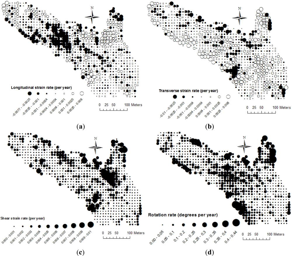
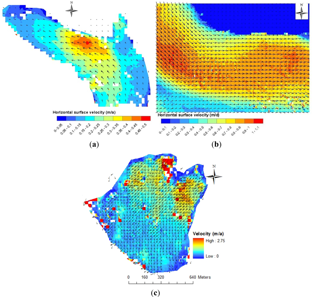
LSM, as a precise matching algorithm, is expected to produce precise velocity for each pixel of the template. This gives the advantage that velocity gradients, i.e., strain rates, can be computed at sub-template level, even if computed after the matching. Additionally, the spatial transformation parameters (
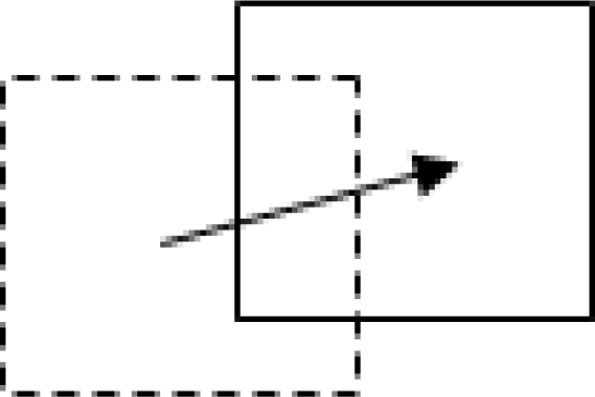
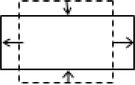
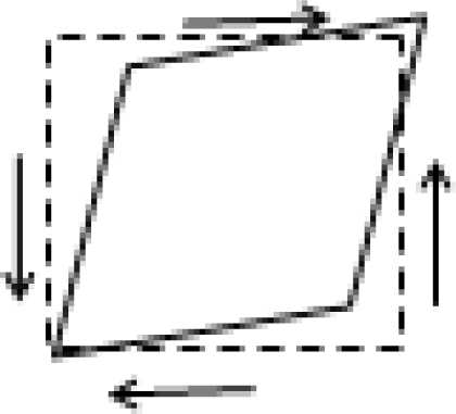
pi) are measures of the geometric deformation of the masses between the acquisition times of the two images. The specific meanings of each of the spatial transformation parameter in mass movements are presented in Table 1 together with a sketch of the geometric changes represented. The spatial transformation parameters can be exploited to automatically compute strain rates simultaneous with the matching as outlined below.
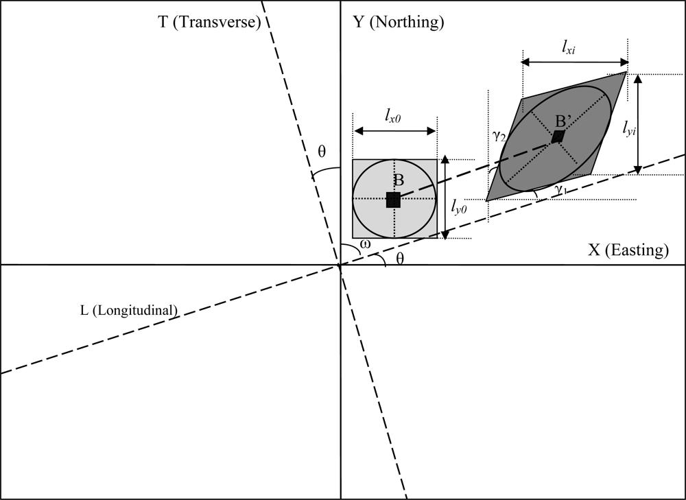
Figure 1 reduces the reality of Earth surface mass movements to the square template depicted, which has unit sizes in both dimensions (denoted as lxo and lyo respectively). The unit lengths can also be thought of as diameters (2r) of a circle as shown in the figure. After deformation, the template moves to a new location, attains new sizes (lxi and lyi) and gets rotated and/or sheared by angles γ1 and γ2 to a new shape. The circle now becomes an ellipse with maximum extension and compression shown orthogonal to each other (dashed axes of the ellipse). The orientation of the ellipse is not necessarily along the movement direction due to shearing and rotation. Notice that the central pixel itself is also deformed and displaced from the center. The Euclidian distance between B and B′ (parallel to the longitudinal direction) is the horizontal displacement magnitude while ω is the angular displacement direction measured clockwise from the north. The change in size can be quantified using extension ratios (Sx and Sy) as in Equations (9) and (10). Sx and Sy are the same as the scaling factors p2 and p6 of Table 1. The corresponding normal strains (εx and εy) and their relations with the scaling factors are given in Equations (11) and (12), adapted from [22,23]. Scaling factors greater than 1 (i.e., εx and εy values greater than 0) imply extension, where as scaling factors less than 1 (i.e., εx and εy values less than 0) imply compression.
The tangent of the shearing angle or the angle in radians (as the angles are often very small) for each direction is the same as the shearing factors (p3 and p5) of the transformation models. Shear results in both shearing and rotation. Thus, shear strain (γxy) and rotation angle (φxy) are derived from the shearing angles as given in Equations (13) and (14) respectively [24]. Strain is better expressed in terms of strain rate (ɛ̇i) which is strain per unit time (Equation (15)). The strain rates in this study are expressed in the time unit that is covered by the dataset in order to avoid extrapolating to time periods not supported by data.
S x = l xi l xo
S y = l yi l yo
ε x = l xi l xo l xo = S x 1
ε y = l yi l yo l yo = S y 1
γ xy = 1 2 ( γ 1 + γ 2 )
φ xy = 1 2 ( γ 1 γ 2 )
ɛ ˙ i = ε i t 2 t 1
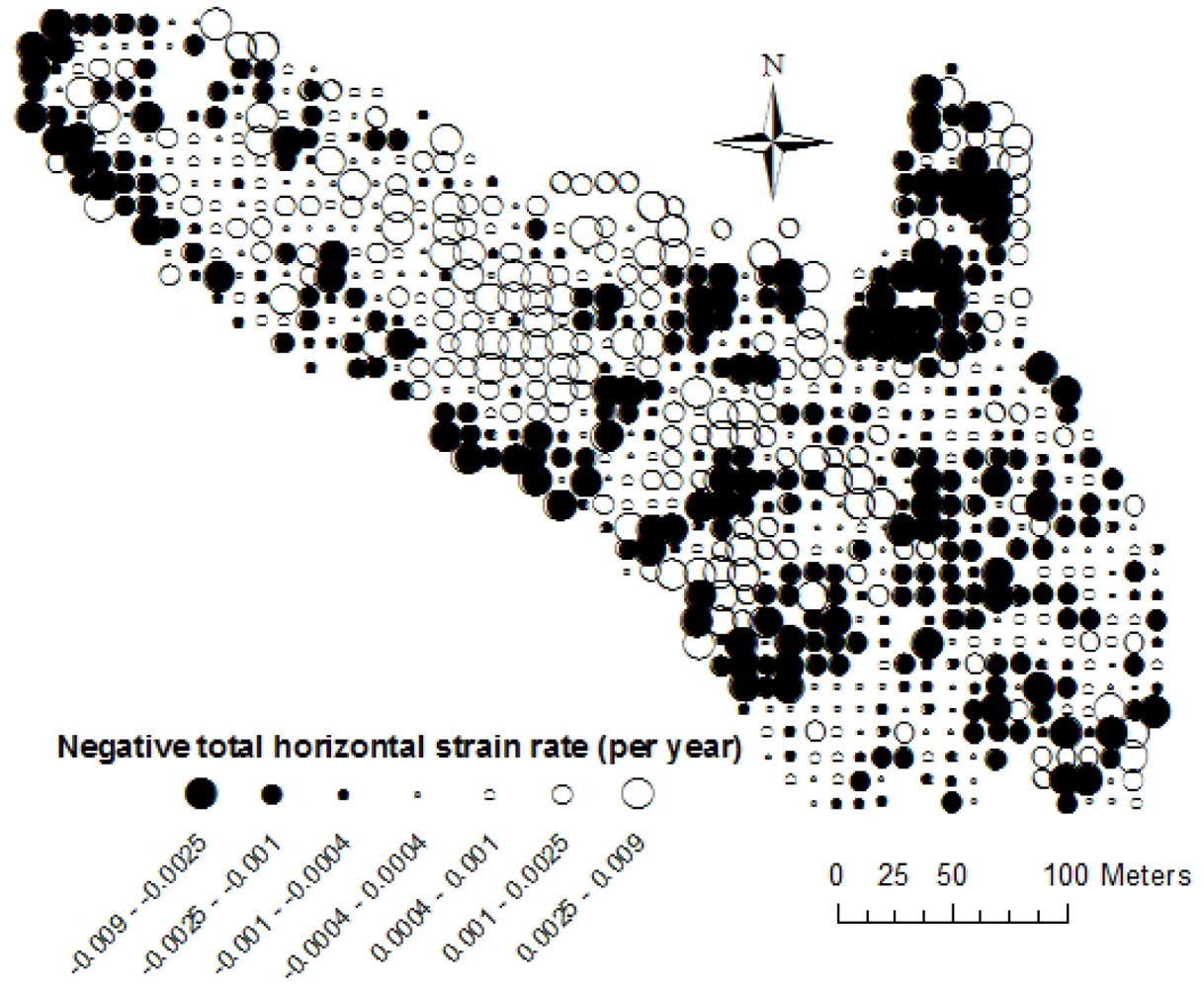
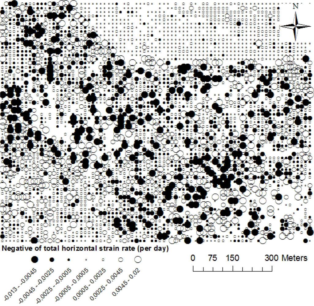
The horizontal length of the ground surface plane changes when there is compression or extension. As ice is incompressible, and thus also to a large extent masses that are super-saturated with ice, horizontal compression is usually balanced by vertical extension or vice versa [25], making the total sum of the horizontal and vertical strain rates equal to zero. Compressive/extending motion is well discussed for glaciers [24,26,27] and rockglaciers [25,28,
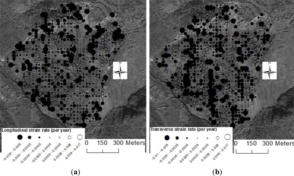
29]. In all cases, longitudinal (i.e., along the flow direction) and transverse (i.e., across flow direction) extension and compression are mentioned to lead to such processes as the formation of crevasses, calving and surface micro-topography. Shearing may lead to cracking of the masses and eventually collapses.
In this study, the radiometric parameters are not used further than estimation of the matching position although it can potentially be used in estimation of surface albedo changes.

3. Methods

3.1. Image Datasets

In this study, the computations were conducted on three real mass movement image pairs and two pairs of simulated deformed images. The first bi-temporal set of images (Figure 2) was taken over a rockglacier in the Muragl valley of the Upper Engadine area in the Swiss Alps (approx. 9.92°E, 46.50°N). The orthoimages used in the present study were based on aerial images taken on 7 September 1981 and 23 August 1994 with 13 years of temporal baseline and 0.2 m of spatial resolution. The Muragl rockglacier has been under investigation for decades using technologies such as photogrammetry, geodesy and geophysics to understand its mechanics [30,31].
The second image pair is a section from panchromatic aerial images over the Nigardsbreen glacier in Southern Norway (approx. 61.68°N, 7.20°E). The images were acquired on 19 and 29 August 2001 within the EU Glaciorisk project (Figure 3). The images were orthorectified using photogrammetric stereo pairs and automatic DEM extraction of the two dates. The ground resolution of the orthoimages is 0.3 m. Surface changes within the very short time period of 10 days were very small, besides glacier flow. Additional details on the images and on their glaciological analysis can be found in [32].
The third bi-temporal image set (Figure 4) is from panchromatic images taken by the high spatial resolution QuickBird satellite over the La Clapière landslide (approx. 44.25°N, 6.94°E,) in the French Alps near the town of Saint-Etienne-de-Tinée. The first image was taken on 6 September 2003 with a mean in-track view angle of −0.5° and a mean cross-track off-nadir view angle of 9°; whereas, the second image was taken on 27 September 2010 with a mean in-track view angle of −0.4° and a mean cross-track off-nadir view angle of 4.2°. The ground pixel size of the images is 0.6 m. The images were orthorectified in PCI-Geomatica using the SRTM DEM and GCPs collected from stable areas based on the French 3D web service ( www.geoportail.fr). As the orthorectification based on this base-map could not result in accurate co-registration, subsequent co-registration using polynomial transformation model was performed using precise GCPs collected from outside the landslide area. Finally, a mean co-registration error of about 1.2 m (2 pixels) is recorded from the horizontal shifts outside the landslide area. The La Clapière landslide has been intensively investigated over the years using different techniques [3,3335].
A simulated image pair was created by analytically deforming a section of the Nigardsbreen aerial photographic image by using an affine geometric model. Gaussian noise of mean zero and variance (σ2n) 0.01 was added. Another simulated image pair was created by using the same deformation model but adding a higher level of noise, σ2n of 0.1. The two simulated deformation image pairs are used for the evaluation of the algorithm as the actual displacements and transformation parameter values are precisely known for these images, in contrast to the real mass movement images.

3.2. Image Matching

3.2.1. Estimation of Initial Parameters

Considering older images as reference and newer images as search images, the images are first matched using the pixel-precision NCC algorithm to estimate the initial model parameters for the least squares adjustment. Initially, the matching templates are assumed to have the same geometry (except position). Therefore, for each dimension a unit geometric and radiometric scaling factor is used keeping the other parameters at zero. The least squares iteration starts by using these initial values. Template sizes of 51 by 51 pixels are used for the matching. Smaller template sizes were not used to suppress noises and avoid ambiguity. As LSM is applied in a later step, the presence of displacement gradients in such large templates is not of concern, or even desired as we aim at deformation measurement in addition to displacement. In fact, as the images are of high resolution, the templates are not large in ground size, i.e., 10.2 m, 15.3 m and 30.6 m for the rockglacier, glacier and landslide images respectively. The search distance is decided based on the expected maximum displacement in each of the image pairs.

3.2.2. Least Squares Iteration

LSM is implemented using the affine transformation model following the procedures explained in Section 2.1. The gradients are computed from the matching template, not from the reference template. Intensity values at sub-pixel positions are interpolated using the cubic convolution [36] as it is the closest to the sinc interpolation, which is considered the most accurate in image interpolation [37]. The limit for the convergence of the parameters except the translation of the gray-values is set to 10−4 for the glacier and the rockglacier, but 10−3 for the landslide due to the presence of more noise resulting from the vegetation cover and orthoprojection errors. The maximum number of iterations is set to 30 for cases where the parameters do not converge faster. In all cases, when the number of iteration reaches 30 the values of each adjustment should be less than 10−1. After the convergence, the cross-correlation coefficient between the two matching templates should be greater than that of the initial. The SSD between the two templates should now be below that of the initial. Otherwise, the template is considered incorrectly converging, i.e., a mismatch, and excluded from the further analysis.

3.3. Computation of Displacement and Deformation

3.3.1. Horizontal Surface Displacement

After the parameters have converged, the horizontal surface displacement of each pixel is computed separately as Euclidian distance between the pixels’ positions in the reference and the matching templates. Velocity is then computed as the displacement divided by the temporal baseline of the image pair. The movement direction is computed as the arctangent of the ratio of the displacements of the easting and northing directions in angles from the north. For later comparison, the displacements for each mass movement are also registered for the pixel-precision NCC. The mean and standard deviation of the velocities are computed. The standard deviation is computed as the square root of the sum of square differences between individual values and the mean divided by the total number of observations.

3.3.2. Surface Strain and Rotation Rates

The transformation parameters are computed for the X (easting) and Y (northing) directions of the image. However, strains of Earth surface masses have plausible meaning when computed along (longitudinal) and across (transverse) the displacement direction. Therefore, the parameters computed for the easting and northing of the images are transformed to the longitudinal (L) and transverse (T) parameters (Figure 1). First, however, the coefficients of the spatial transformation models are converted to strain parameters as explained in Section 2.2. As the parameters are measures of components of the strain tensor, we use strain transformation equations [2224]. The strain parameters are thus transformed to the axis along the displacement direction (L), i.e., θ degrees from the X-axis, and across the displacement direction (T), i.e., θ degrees from the Y-axis. εx, εy and γxy are then used to compute εL (longitudinal strain), εT (transverse strain) and γTL (shear strain) as in Equations 1618 respectively. The computations are included in the MATLAB code that is used for the matching to automatically compute the strain rates and rotation angles in addition to the displacement. For the glacier and rockglacier, the negative values of the sums of the longitudinal and transverse strain rates are computed to estimate the vertical strain rate (Equation (19)) as both masses are assumed to be incompressible. All of the results are then mapped for visualization and interpretation.
ε L = ε x cos 2 θ + ε y sin 2 θ + γ xy sin θ cos θ
ε T = ε x sin 2 θ + ε y cos 2 θ γ xy sin θ cos θ
γ TL = 2 ( ε x ε y ) sin θ cos θ + γ xy ( cos 1 θ sin 1 θ )
ε z = ( ε L + ε T )

3.4. Performance Evaluation

The precision of the LSM algorithm in matching and computation of displacement and strains are evaluated using error propagation principles [18,38]. The precision of the estimated parameters can be expressed by the covariance matrix (Equation (20)). However for the precision of the matching, Gruen [18] suggests the use of the standard deviation of the shift parameters alone (Kp1 and Kp4) as they determine how precise the matching position is (Equation (21)). Precision measures based on the covariance matrix are however known to be optimistic due to the high data redundancy [16,18].
K xx = σ 0 2 Q xx = σ 0 2 ( A π A ) 1
K pi = σ ^ pi = σ 0 ( Q pi ) 1 / 2
Accuracy (validity) assessment of the measurements such as displacement and strain rates is conducted on stable grounds and simulated deformation images. The stable grounds are expected to have zero values for the displacement, strain rates and rotation. Simulated deformed images have known displacement and deformation parameter values. The mean absolute deviation (MAD) between the actual and the computed values is used for the evaluation. Stable grounds are, however, not a complete representation for the mass movements as one source of error, which is the deformation, does strictly speaking not exist on the stable ground. Thus, to compare the performance of the algorithm over the moving masses to that of the NCC, the SNR of reconstructing the reference image from the search image is computed as detailed in [39], assuming that accurate matching leads to accurate reconstruction. The SNR is computed as the ratio between the correlation coefficient (ρ) and 1 − ρ. The relative gain of the SNR is used as a measure of relative performance.

4. Results

4.1. Horizontal Surface Displacements

The horizontal surface velocity statistics of the three mass movements investigated is presented in Table 2 to give an overview of the mean, standard deviation (variation of the magnitudes) and the maximum values of the horizontal surface velocities of the mass movements. The velocities of the rockglacier and the landslide are in the range of (tens of) centimeters per year while that of the glacier is in the range of centimeters per day or meters per year (ma−1). In the table, we use velocity units that are relevant for the time period covered by the image pairs. For example, we use md−1 as opposed to ma−1 for the velocity of the Nigardsbreen as the data cover only 10 days from late summer. The data on maximum velocity, especially those of the landslide, needs to be read with caution. Experience shows that in image matching, ambiguous (noise-based) matches often lead to large displacement estimates. Even when they are filtered manually and systematically, some of such false matches would still remain. Mismatches often occur in fast moving areas where surface destruction is likely. Although such outliers may not have considerable influence on the mean, they may inflate the maximum values.
The velocity magnitude map of the Muragl rockglacier computed using the LSM is presented in Figure 5(a) with the velocity vectors overlaid. The tongue-like shape of the rockglacier also manifests in its velocity distribution creating a similar pattern. The mean velocity of the rockglacier is computed to be 0.18 ma−1, with the maximum reaching up to 0.50 ma−1. The area with highest speeds in the middle of the rockglacier causes considerable velocity gradients. Upstream of this area velocity increases significantly while velocity decreases downstream along the creep direction. The smooth transitions in the velocity field instead of stepwise ones are ascribed to the capability of the LSM to detect and estimate intra-template displacement variation unlike the constant displacement assumed for each template by the NCC-based matching, for instance. The displacement voids in the figure indicate templates that failed to converge during the LSM iteration.
Figure 5(b) presents the spatial variation of velocity on the Nigardsbreen glacier computed using the LSM with the velocity vectors overlaid. The glacier velocity is high in the center decreasing towards the boundaries. The velocity vectors show a coherent field of flow directions.
The velocity magnitude map of the La Clapière landslide is presented in Figure 5(c) together with the velocity vectors. The upper part of the landslide moves faster than the lower. The recently detached part on the upper left part is also moving with high velocity. The reliability of matches in this area is, however, questionable as it is close to the head scarp of the landslide where significant surface changes are likely to lead to mismatching. The velocity vectors show that the major part of the landslide moves towards the south-west with its lower part turning slightly to the south-east direction.

4.2. Precision and Validity of the Displacement Data

Table 3 presents the precision of the shift parameters of the three mass movements averaged over all templates. The highest precision is recorded for the Muragl rockglacier image while the lowest is recorded for the La Clapière landslide. The mean precision ranges between about 1/20th of a pixel (Muragl) to 1/6th of a pixel (La Clapière). These values show the power of LSM in locating the matching positions under different radiometric and geometric distortions. After consultation of their histograms, templates with precision of the shift parameters over 0.2 were removed from the analyses. The accuracy (validity) is however dependent on the precision of the precision of the orthorectification and co-registration of the images, deformation of the templates, and noise. Stable grounds and simulated deformation images are used to evaluate the validity of the LSM and the NCC algorithms.
Table 4 presents the mean absolute deviation (MAD) between the measured displacement and the expected displacement for the simulated images and the stable grounds of real mass movements. For the simulated image with low noise variance, about 90% reduction in MAD by the LSM compared to that of the pixel-precision NCC is obtained. However, when σ2n is raised to 0.1, the reduction in the MAD by the LSM from that of the NCC is only 52%. When the noise level (σ2n) increased ten-fold, the error in the estimated displacement increases five-fold for the LSM and only 10% for the NCC. We do not investigate further at this point how far this trend is a general one for LSM applied to noisy images. However, the finding supports the widely known general robustness of the NCC algorithm with regard to noise. The reduction in the MAD of displacement error on the stable grounds of the real mass movements is also presented. As the table shows, the MAD is the lowest for the glacier (due to precise orthorectification and co-registration of the images) and the highest for the landslide. The percentage of the error (MAD) of the NCC reduced by the use of LSM is the highest in the Muragl rockglacier case followed by the glacier and the landslide respectively.
As stated above, the SNR of reconstructing the reference image of t1 from the deformed image of t2 is also computed over the mass movements. For the analytically deformed image pairs, the relative gain in the SNR of the LSM in relation to that of the NCC is close to 100% (double) in the case where the noise standard deviation is 0.01 and 47% where it is 0.1. For the real mass movement images, around 25% gain in SNR of matching is obtained by using the LSM compared to that of the NCC. The LSM algorithm again makes the best improvement on the Muragl rockglacier. The expectation is that this improvement in the SNR of the image reconstruction translates to improvements in the precision of the estimated displacements (and thus velocities). For the analytically deformed images, the gain in the SNR is comparable to the reduction in MAD of the estimated velocities. The improvements in the SNR for the real mass movements are also comparable to the reductions in the MAD of the velocities on stable ground except for the La Clapière landslide. The general trend of agreement between the SNR gain and the reduction in MAD of displacement shows some important points. (1) The LSM performs clearly better than the NCC. (2) The SNR gain of image reconstruction is directly related to the precision of the displacement estimation. (3) Increased noise level reduces the performance of the LSM, which strongly indicates that the LSM is more sensitive to noise than NCC.

4.3. Surface Strain and Rotation Rates

4.3.1. The Muragl Rockglacier

The deformation parameters investigated in this study are the longitudinal strain rate (ɛ̇L), the transverse strain rate (ɛ̇T), the shear strain rate (ɛ̇LT) and the rotation rate (φ̇). The results for the Muragl rockglacier are presented in Figures 6 and 7. Summary statistics for the computed deformation parameters are given in Table 5. The statistics of the ɛ̇L data shows that 96% of the creeping rockglacier has ɛ̇L between −0.0034 a−1 and 0.0037 a−1 with a mean of 0.00012 a−1. Regions of extending deformation (the hollow circles of Figure 6(a)) are regions where the velocity increased considerably over short distance. Areas of compressive movement (black circles in the figure) are characterized by decreasing speed along the creep direction. One region stands out for its high compression in the longitudinal direction. This region is located immediately downstream of the high velocity region shown in the velocity map (Figure 5(a)). The rest of the rockglacier is characterized by steady creep with very limited velocity gradients.
The ɛ̇T map (Figure 6(b)) shows that the rockglacier is compressed where velocity decreases across the flow direction and extended where velocity increases across the flow direction obeying a similar rule as ɛ̇L. The figure shows that the rockglacier is mainly extended in the transverse direction. The extension is more pronounced in areas where longitudinal compression is recorded. In contrast to the ɛ̇L, the upper (northern) side of the tongue-like shape of the rockglacier is mainly compressed in transverse direction, while the lower boundaries are mainly extended.
The horizontal compression and extension are compensated for by the vertical extension and compression respectively as the rockglacier can roughly be assumed to be incompressible due to its substantial ice content. This means the negative sum of the horizontal strain rates presented in Figure 7 is assumed to be equal to the vertical strain rate. The upstream part of the rockglacier and its margin at the tip of the tongue-like shape are dominated by vertical compression, which would in practice lead to dynamic thinning of the body. This is indicative of net material drainage from that zone into the lower one. The downstream part of the rockglacier is dominated by vertical extension (hollow circles of the figure) or horizontal compression indicating net influx of material, and expected dynamic thickening. However, erosion of materials, vertical compression, at the tip of the tongue-shaped rockglacier is clearly marked by the dark circles of Figure 7.
The ɛ̇LT of the Muragl rockglacier (Figure 6(c)) demonstrates high shear strain rate associated with the boundaries of significant change in velocity (speed or direction) as can be observed from the regions of the figure where black circles dominate. The significant change in flow direction and speed seems to have created such significant shearing. The mean ɛ̇LT is 0.0015 a−1, which means 1.5 mm of shearing in a 1 m horizontal distance over a one year period. However, this parameter value can in places reach up to 1 cm (Figure 6(c) and Table 5).
Figure 6(d) presents the spatial variation of the rotation rate for the rockglacier. The high rotation areas are the inflection zones where the rockglacier flow direction changes from the northward to the north-westward. The maximum rotation rate registered is 0.44 degrees a−1 with the mean rotation rate close to 0.07 degrees a−1. The strain, shear and rotation values obtained are representative for the size of matching windows used, here 51 × 51 pixels. The values may change slightly with template size as the spatial transformation parameters are for the whole template.

4.3.2. The Nigardsbreen Glacier

Summary statistics of the computed deformation parameters for the Nigardsbreen glacier (maps not shown here) are given in Table 6. The statistics here include stable ground which has deformation parameter values close to zero. Recalling that ice is not compressible, the negative of the sum of the longitudinal and the transverse strain rates is computed for the Nigardsbreen and presented in Figure 8. A major part of the glacier section registered total horizontal compression (vertical extension), i.e., dynamic thickening of the glacier. The stable ground (upper right) is unstrained and thus has vertical strain rates close to zero. The boundaries with the stable ground are compressed in transverse direction which is not compensated with longitudinal extension. Therefore, it is vertically extended or thickens dynamically; so are all the areas shown in hollow circles. The areas covered by the dark circles are areas where the glacier has shown horizontal extension. As stated above, vertically extended areas indicate dynamic mass gain while vertically compressed areas indicate dynamic mass loss. Notice that the data voids in the figure are results of thresholding the precision of the shift parameters at 0.2.

4.3.3. The La Clapière Landslide

The computed ɛ̇L, ɛ̇T, ɛ̇LT, and rotation rate for the La Clapière landslide are presented in Figure 9(a–d) respectively. Summary statistics of the deformation parameters for the landslide are presented in Table 7. Recall that the images have poor orthorectification quality and the ground undergoes considerable surface changes in seven years due to the vegetation cover. Therefore, the deformations quantified are not necessarily the ground deformation alone. Nonetheless, longitudinally the landslide is mainly extended with few zones of compression (Figure 9(a)). As expected, the lower part of the landslide is longitudinally compressed. There are some interesting regions where significant transverse compression is observed (Figure 9(b)). These areas are where the masses converge from two directions leading to compression or net influx of masses. There are three channel-like compression regions as can be observed from the maps of the ɛ̇T. These patterns however do not have corresponding ground structures. The mass is a porous medium that can change density under stress. Therefore, the principle that holds for glacier and roughly for rockglaciers that compression in one dimension leads to extension in the other dimension does not necessarily hold for such porous landslides. Computing the negative sum of the horizontal strain rates thus does not produce a meaningful parameter.
When it comes to the surface shear strain rate (Figure 9(c)), it is only the north-west and western part of the landslide that is highly sheared. The northwestern part of the landslide cracked from the stable ground recently and seems to be actively shearing. The same regions show high rotation rate (Figure 9(d)). The major part of the landslide seems to be extended both longitudinally and transverse with limited shearing and rotation. Apart from the northern part, the high rotation areas are the foot of the landslide where the materials rotate towards south-east after reaching the foot.

4.4. Precision and Validity of the Deformation Data

Error propagation using the covariance matrix of the geometric parameters of the affine transformation model (Kpi) shows high precision (Table 8). The parameters are related directly to the strains as shown in the bracket. The mean absolute value of the estimated parameters is given in the parenthesis for overview of the relative magnitude of the precisions. The uncertainty is therefore less than 10% of the estimated parameter values, i.e., at least one order of magnitude lower. The scaling parameters are relatively more precise than the shearing parameters.
The MAD of the strain rates on the stable grounds are in the order of 10−4 for the glacier and rock glacier and 10−3 for the landslide (Table 9). This means the values estimated for each deformation parameter in reality lies within the estimated value ± the MAD. The error values for rotation are somewhat higher in all cases. This might be an indication of a slight rotation of one of the images against the other. The error magnitudes are however below (at least one order of magnitude lower than) the estimated values of the deformation (rotation and strain rates) except that of the La Clapière landslide for which the computed strain rates are not significantly outside the error margin. These MAD values can even be optimistic as they are computed on non-deformed area, i.e., stable ground.

5. Discussion

5.1. Computed Displacements and Deformations

Although no formal quantitative comparison is conducted, the velocities obtained for the mass movements using the LSM are in agreement with those obtained in other studies using similar and other methods. For example, similar velocities are registered for the same section of the Nigardsbreen glacier during the same period [32]. The average and maximum velocities of the Muragl rockglacier are similar to what is reported in [30] which is validated using different approaches, including ground measurements. The surface velocity data in [30] agrees well with that of borehole data [40]. The limited surface change during the 13 years period contributes to the success of optical image matching on this rockglacier, and rockglaciers in general. The spatial pattern of the La Clapière landslide velocity variation is in agreement with that computed by other studies, particularly [3]. The velocity magnitudes show a slight slowdown from earlier records (e.g., [33,41]). The decreased magnitudes are in agreement with the general observation of the slowdown of the landslide since the year 2000 ( http://gravitaire.oca.eu/spip.php?rubrique15). Errors in the orthorectification and the presence of vegetation on the surface leading to radiometric noises imply the presence of blunders in the image matching.
Realistic values of longitudinal, transverse and shear strain rates together with rotation rate are also obtained. The technique computes strain rates at higher resolution than the conventional technique of computing them from velocity gradients after the matching. When computing strain rates of a template from the velocity gradients, two neighboring templates are used for each orthogonal dimension. Therefore, the computed negative total sum of strain rate is in a way averaged over neighboring templates. Additionally, such strain rates are simply measures of velocity changes between the central pixels of the neighboring templates especially when the NCC is used for the matching. Thus it can appear smoothed even before filtering. Changes in the size and shape of the masses are not directly computed as is done when using the LSM algorithm as presented here. As a result micro-scale deformations are detected with LSM.
The spatial patterns of the strain rates and elevation changes of the Muragl rockglacier, previously computed from velocity gradients by [8], agree with those of the present study. The negative total of the horizontal strain rates of the present study (Figure 7) agrees with Figure 3 of [8]. Notice that the symbols in the present study and [8] are inverses of each other and scaled differently. Areas of vertical compression (horizontal extension) in our study correspond with negative elevation changes presented in Figure 2 of [8], indicating dynamic loss of mass from the vertically compressed areas. For the Nigardsbreen glacier, the negative sum of the horizontal strain rates shows that the glacier is dominantly extended vertically, which is in agreement with the thickening of the glacier as reported in [32], and with the general ice compression in glacier ablation areas. High shear strain rate is registered at the margins of flow, especially where the moving glacier borders with stable ground. The deformation maps of the La Clapière landslide require cautious interpretation as more sources of error can influence the reliability compared to the other two mass movement types as discussed in the following section. Specifically, propagated orthorectification error and surface changes such as vegetation cover contribute to major blunders in the strain rate data. Computation of strain rates on its stable ground shows that the computed strain rates are not outside the error margin, i.e., not statistically significant.

5.2. On the Precision of the Algorithm and Sources of Error

The results of the study show that the LSM computes horizontal displacements in Earth surface mass movements with significantly higher precision (level of detail of measurement) and accuracy (truthiness of the estimated values) compared to the NCC. The mean precision of the LSM algorithm in locating the matching position is found to be between 0.06 and 0.15 pixel; whereas, the matching precision of NCC without sub-pixel extensions is generally ±0.5 pixel. In addition to the precision of matching, the accuracy of the computed displacements is also higher when computed using LSM than using NCC as evaluated on test images and stable grounds of the bi-temporal mass movement images. The better performance of the LSM is in agreement with theoretical claims and earlier findings in photogrammetry on image pairs of shorter temporal baselines [20,21,42].
When computing deformation and displacement of mass movements from repeat images using a precise algorithm such as LSM, the sources of error are basically related to either the image (noise, orthorectification and co-registration) or the ground itself (deformation and temporal surface changes). Both major error sources can technically be grouped into three, i.e., geometric errors, radiometric errors and propagated sensor or processing errors. The possible sources that cause geometric error are: (1) the formation of crevasses or micro-topography, (2) the boundary effect where the velocity gradient between the moving body and the stable ground is so large that it creates outlying deformation parameter values, (3) vegetation cover can also create geometric change that is not actually ground deformation in addition to its contribution to intensity noise. Signal- (in fact the SNR-) related causes include the presence of shadows, surface changes, illumination differences, presence of dirt, vegetation cover, etc., that can lead to false and outlying convergence parameter values in the least squares iteration. Propagated errors can be attributed to the sensor or image preprocessing, such as orthorectification and co-registration. If the images are not perfectly orthorectified and co-registered, the geometric adjustment includes the mass deformation, sensor projective distortion and change of geometry between the two images [17,43].
Due to the high resolution of strain computation, the maps of the strain rates look noisy when visually observed, suggesting the application of noise filters. However, in the case of the strain rate maps, it might well be that high-resolution deformations actually are somewhat noisy due to real local deformation of the masses, such as from crevasse formation, or due to the error sources mentioned above. Filtering would lead to smoothing of the map. In so doing it affects both the realistic values and the blunders. The use of larger template sizes also leads to a more smoothed strain rate map. Recall that the criteria for the right template size in the NCC is the presence of adequate SNR and constant displacement within the template. In the LSM, constant displacement is not anymore a criteria but rather a constant displacement gradient, at least for the affine model. Thus, for very large templates, as the parameters of the transformation model are forced to be constant within the template, the computed strain rates visually look like as if they are filtered. Such smoothed or filtered strain rate map may be sufficient or even wanted for some geoscientific applications such as numerical models. However, the detailed variability may be needed for other current and future applications, and provide new insights into the mechanics of mass movements.
A better approach towards removing noises than filtering or the use of much larger template sizes would therefore be further restricting the least squares iteration process. Pixel-based constraining such as data snooping or template-based constraining such as raising convergence precision can be used [18,21]. This would affect only the highly noisy (and maybe the highly deformed) templates, leaving the well-converging templates unaffected. An initial test shows that increasing the demanded precision of the parameter adjustment during the LSM iteration discards more templates, resulting in more data voids. However, the strong spatial variability is not substantially smoothed, implying that it stems from real strain rate variations.

6. Conclusions and Outlook

This study explored the possibility of automatically and simultaneously computing displacement, strain rates and rotation of Earth surface mass movements from repeat high resolution satellite and aerial optical images. The performance of least squares matching (LSM) with an affine geometric transformation model is evaluated in relation to that of the most widely used algorithm for such purposes, i.e., the normalized cross-correlation (NCC). Aerial and high spatial resolution satellite images over glacier flow, rockglacier creep and land sliding are used in the study covering three different types of mass movements and two different types of imaging systems.
The results of the study clarified that the LSM estimates the displacement of Earth surface masses with better precision and accuracy than the conventional NCC. Around 25% improvement in the SNR gain of image matching over that of the NCC is registered in real images reaching up to double in the case of the analytically deformed images. The improvements in the SNR gain lead to comparable improvements in the accuracy of the estimated displacement. Up to 35% reduction in the MAD of displacement by the LSM from that of the NCC is observed on the stable grounds of the mass movement images reaching up to 90% in the case of the simulated deformation. The exact magnitude obviously varies depending on the application scenario. The improvements are dependent on the level of noise in the images.
The study has also demonstrated the capability of the LSM in deriving surface strain rates and rotation rate simultaneously with the image matching process. This has the potential of replacing earlier approaches based on post-processing from displacement gradients. Additionally, the spatial density of deformation parameters measured, and thus the unprecedented level of detail of deformation fields obtained, might allow for new insights into the mechanics of the masses observed. The strain rate data obtained through such processes are found to be realistic when compared with data from different sources and when logically evaluated. The spatial transformation parameters from which the strain rates are derived are computed with precisions better than 10% of the measured values in all cases. However, evaluation of the accuracy (validity) of the rotation and strain rates on the stable grounds of the mass movement images shows that the accuracy is dependent on the mass movement type, i.e., image and ground characteristics. The MAD is as low as 10−4 for the rockglacier and the glacier (one order of magnitude smaller than the computed average strain rates, i.e., 10% as well). For the landslide, the computed strain rates do not exceed their error margins.
The capability of deriving surface strains from images through the LSM algorithm advances the application of image matching in mass movement analysis. Once strain is reliably computed from repeat images automatically through image matching, the stress exerted on the masses can also be computed using the stress-strain relationship for the specific type of mass under investigation. This is very important in early warning related to slope instabilities and failures, and in understanding terrain kinematics, and potentially dynamics, in high mountain areas. Nevertheless, validation of the computed strain under different conditions and possibility of extending to the computation of stress requires further research.
The algorithm is computationally expensive as it involves iteration for each template. The ever improving computer processor speeds coupled with smarter computational approaches can deal with this limitation. Initial tests indicate that the algorithm is very sensitive to noises in the images. More work is thus needed to define the sensitivity and applicability range of the LSM approach for repeat images of lower resolution, of more strongly deforming masses, and with longer temporal baselines.

Acknowledgments

The orthoimages of the Muragl rockglacier are based on aerial photos acquired by the Swisstopo/flight service (BA057212, BA081844). The Nigardsbreen aerial images are courtesy of EU Glaciorisk. This study is funded by the Research Council of Norway (NFR) through the CORRIA project (no. 185906/V30) and contributes to the NFR International Centre for Geohazards (SFF-ICG 146035/420), the ESA Glaciers_cci project (4000101778/10/I-AM), and the Nordic excellence center SVALI. The QuickBird images are courtesy of DigitalGlobe. Special thanks go to the anonymous referees, and to Editor-in-Chief, Prasad Thenkabail for the comments that substantially improved the paper. We would like to thank Kimberly Casey for proofreading the manuscript.

References

  1. Kääb, A.; Haeberli, W.; Gudmundsson, G.H. Analysing the creep of mountain permafrost using high precision aerial photogrammetry: 25 years of monitoring Gruben rock glacier, Swiss Alps. Permafrost Periglac. Process 1997, 8, 409–426. [Google Scholar]
  2. Bindschadler, R.A.; Scambos, T.A. Satellite-image-derived velocity field of an Antarctic ice stream. Science 1991, 252, 242–246. [Google Scholar]
  3. Delacourt, C.; Allemand, P.; Casson, B.; Vadon, H. Velocity field of the “La Clapière” landslide measured by the correlation of aerial and Quickbird satellite images. Geophys. Res. Lett 2004, 31, 15–19. [Google Scholar]
  4. Rolstad, C.; Amlien, J.; Ove Hagen, J.; Lundén, B. Visible and near-infrared digital images for determination of ice velocities and surface elevation during a surge on Osbornebreen, a tidewater glacier in Svalbard. Ann. Glaciol 1996, 24, 255–261. [Google Scholar]
  5. Berthier, E.; Vadon, H.; Baratoux, D.; Arnaud, Y.; Vincent, C.; Feigl, K.L.; Remy, F.; Legresy, B. Surface motion of mountain glaciers derived from satellite optical imagery. Remote Sens. Environ 2005, 95, 14–28. [Google Scholar]
  6. De Matías, J.; De Sanjosé, J.; López-Nicolás, G.; Sagüés, C.; Guerrero, J. Photogrammetric methodology for the production of geomorphologic maps: Application to the Veleta rock glacier (Sierra Nevada, Granada, Spain). Remote Sens 2009, 1, 829–841. [Google Scholar]
  7. Zitová, B.; Flusser, J. Image registration methods: A survey. Image Vision Comput 2003, 21, 977–1000. [Google Scholar]
  8. Kääb, A.; Kaufmann, V.; Ladstadter, R.; Eiken, T. Rock Glacier Dynamics: Implications from High-Resolution Measurements of Surface Velocity Fields. Proceedings of the 8th International Conference on Permafrost, Zurich, Switzerland, 21–25 July 2003; pp. 501–506.
  9. Kääb, A. Remote Sensing of Mountain Glaciers and Permafrost Creep. 2005; p. 264. [Google Scholar]
  10. Brown, L.G. A survey of image registration techniques. ACM Comput. Surv 1992, 24, 325–376. [Google Scholar]
  11. Lewis, J.P. Fast normalized cross-correlation. Vision Interface 1995, 120–123. [Google Scholar]
  12. Debella-Gilo, M.; Kääb, A. Sub-pixel precision image matching for measuring surface displacements on mass movements using normalized cross-correlation. Remote Sens. Environ 2011, 115, 130–142. [Google Scholar]
  13. Förstner, W. On the Geometric Precision of Digital Image Correlation. Proceedings of the ISPRS Symposium Mathematical Models, Accuracy Aspects and Quality Control, Finland; 1982; pp. 176–189. [Google Scholar]
  14. Schenk, T. Digital Photogrammetry; TerraScience: Laurelville, OH, USA, 1999; Volume I, p. 428. [Google Scholar]
  15. Whillans, I.M.; Tseng, Y.H. Automatic tracking of crevasses on satellite images. Cold Reg. Sci. Technol 1995, 23, 201–214. [Google Scholar]
  16. Maas, H.G.; Casassa, G.; Schneider, D.; Schwalbe, E.; Wendt, A. Photogrammetric determination of spatio-temporal velocity fields at glaciar San Rafael in the northern Patagonian icefield. The Cryosphere Discuss 2010, 4, 2415–2432. [Google Scholar]
  17. Kaufmann, V.; Ladstädter, R. Quantitative Analysis of Rock Glacier Creep by Means of Digital Photogrammetry Using Multi-Temporal Aerial Photographs: Two Case Studies in the Austrian Alps. Proceedings of 8th International Conference on Permafrost, Zurich, Switzerland, 21–25 July 2003; pp. 525–530.
  18. Gruen, A. Least squares matching: A fundamental measurement algorithm. In Close Range Photogrammetry and Machine Vision; Atkinson, K.B., Ed.; Whittles Publ.: Caithness, Scotland, UK, 1996; pp. 217–255. [Google Scholar]
  19. Bethmann, F.; Luhmann, T. Least-Squares Matching with Advanced Geometric Transformation Models. In International Archives of Photogrammetry, Remote Sensing and Spatial Information Sciences, Proceedings of ISPRS Commission V Mid-Term Symposium “Close Range Image Measurement Techniques”, Newcastle upon Tyne, UK, 21–24 June 2010; 2010. WG V/4:. pp. 86–91. [Google Scholar]
  20. Gruen, A.W.; Baltsavias, E.P. High-precision image matching for digital terrain model generation. Photogrammetria 1987, 42, 97–112. [Google Scholar]
  21. Rosenholm, D. Least squares matching method: Some experimental results. Photogramm. Rec 1987, 12, 493–512. [Google Scholar]
  22. Young, W.C.; Budynas, R.G.; Roark, R.J. Formulas for Stress and Strain; McGraw-Hill: New York, NY, USA, 2002; p. 852. [Google Scholar]
  23. Middleton, G.V.; Wilcock, P.R. Mechanics in the Earth and Environmental Sciences; Cambridge University Press: Cambridge, UK, 1994; p. 459. [Google Scholar]
  24. Hooke, R.L. Principles of Glacier Mechanics; Cambridge University Press: Cambridge, UK, 2005; p. 429. [Google Scholar]
  25. Haeberli, W.; Hallet, B.; Arenson, L.; Elconin, R.; Humlun, O.; Kääb, A.; Kaufmann, V.; Ladanyi, B.; Matsuoka, N.; Springman, S.; et al. Permafrost creep and rock glacier dynamics. Permafrost Periglac. Process 2006, 17, 189–214. [Google Scholar]
  26. Nye, J.F. The mechanics of glacier flow. J. Glaciol 1952, 2, 82–93. [Google Scholar]
  27. Nye, J.F. A method of determining the strain-rate tensor at the surface of a glacier. J. Glaciol 1959, 3, 409. [Google Scholar]
  28. Kääb, A.; Reichmuth, T. Advance mechanisms of rock glaciers. Permafrost Periglac Process 2005, 16, 187–193. [Google Scholar]
  29. Kneisel, C.; Kääb, A. Mountain permafrost dynamics within a recently exposed glacier forefield inferred by a combined geomorphological, geophysical and photogrammetrical approach. Earth Surf. Proc. Land 2007, 32, 1797–1810. [Google Scholar]
  30. Kääb, A.; Vollmer, M. Surface geometry, thickness changes and flow fields on creeping mountain permafrost: Automatic extraction by digital image analysis. Permafrost Periglac. Process 2000, 11, 315–326. [Google Scholar]
  31. Kääb, A. Monitoring high-mountain terrain deformation from repeated air- and spaceborne optical data: Examples using digital aerial imagery and ASTER data. ISPRS J. Photogramm 2002, 57, 39–52. [Google Scholar]
  32. Wangensteen, B.; Tønsberg, O.M.; Kääb, A.; Eiken, T.; Hagen, J.O. Surface elevation change and high resolution surface velocities for advancing outlets of Jostedalsbreen. Geografiska Annaler: Series A 2006, 88, 55–74. [Google Scholar]
  33. Casson, B.; Delacourt, C.; Baratoux, D.; Allemand, P. Seventeen years of the “La Clapière” landslide evolution analysed from ortho-rectified aerial photographs. Engineering Geology 2003, 68, 123–139. [Google Scholar]
  34. Lebourg, T.; Binet, S.; Tric, E.; Jomard, H.; El Bedoui, S. Geophysical survey to estimate the 3D sliding surface and the 4D evolution of the water pressure on part of a deep seated landslide. Terra Nova 2005, 17, 399–406. [Google Scholar] [Green Version]
  35. Chemenda, A.I.; Bois, T.; Bouissou, S.; Tric, E. Numerical modelling of the gravity-induced destabilization of a slope: The example of the La Clapière landslide, southern France. Geomorphology 2009, 109, 86–93. [Google Scholar]
  36. Keys, R.G. Cubic convolution interpolation for digital image processing. IEEE Trans. Acoust. Speech 1981, 29, 1153–1160. [Google Scholar]
  37. Dodgson, N.A. Image Resampling; University of Cambridge Computer Laboratory: London, UK, 1992; p. 264. [Google Scholar]
  38. Förstner, W. Reliability analysis of parameter estimation in linear models with applications to mensuration problems in computer vision. Comput. Vis. Graph 1987, 40, 273–310. [Google Scholar]
  39. Debella-Gilo, M.; Kääb, A. Locally adaptive template sizes for matching repeat images of earth surface mass movements. ISPRS J. Photogramm 2011. submitted.. [Google Scholar]
  40. Arenson, L.; Hoelzle, M.; Springman, S. Borehole deformation measurements and internal structure of some rock glaciers in Switzerland. Permafrost Periglac. Process 2002, 13, 117–135. [Google Scholar]
  41. Guglielmi, Y.; Cappa, F.; Binet, S. Coupling between hydrogeology and deformation of mountainous rock slopes: Insights from La Clapière area (southern alps, france). Comptes Rendus Geosciences 2005, 337, 1154–1163. [Google Scholar]
  42. Ackermann, F. Digital image correlation: Performance and potential application in photogrammetry. Photogramm. Rec 1984, 11, 429–439. [Google Scholar]
  43. Leprince, S.; Barbot, S.; Ayoub, F.; Avouac, J.P. Automatic and precise orthorectification, coregistration, and subpixel correlation of satellite images, application to ground deformation measurements. IEEE Trans. Geosci. Remote Sens 2007, 45, 1529–1558. [Google Scholar]
Figure 1. Deformation of a template and transformation of its parameters from easting-northing to longitudinal-transverse axis.
Remotesensing 04 00043f1
Figure 2. A section of the aerial photographic image (400 m × 600 m) over part of the Muragl rockglacier taken on 7 September 1981, North to the top.
Remotesensing 04 00043f2
Figure 3. A section of the aerial photographic image (1,233 m × 1,233 m) over part of the Nigardsbreen taken on 19 August 2001, North to the top.
Remotesensing 04 00043f3
Figure 4. A section of the QuickBird panchromatic satellite image (1,600 m × 2,430 m) over the La Clapière landslide taken on 06 September 2003, North to the top.
Remotesensing 04 00043f4
Figure 5. Velocity (ma−1) maps and vectors of (a) the Muragl rockglacier, (b) the Nigardsbreen glacier and (c) the La Clapière landslide computed using the LSM.
Remotesensing 04 00043f5
Figure 6. The longitudinal ɛ̇L (a), transverse ɛ̇T (b), and shear ɛ̇LT (c) strain rates and the rotation rate φ̇ (d) for the Muragl rockglacier.
Remotesensing 04 00043f6
Figure 7. The negative sum of the horizontal strain rates (assumed to be equal to the vertical strain rate for an incompressible medium) for the Muragl rockglacier.
Remotesensing 04 00043f7
Figure 8. The negative sum of the horizontal strain rates (assumed to be equal to the vertical strain rate) of the Nigardsbreen glacier.
Remotesensing 04 00043f8
Figure 9. The longitudinal ɛ̇L (a), transverse ɛ̇T (b), and shear ɛ̇LT (c) strain rates and the rotation rate φ̇ (d) for the La Clapière landslide.
Remotesensing 04 00043f9aRemotesensing 04 00043f9b
Table 1. Parameters of the spatial transformation models related to mass movement processes.
Transformation Parameters of Equations (3) and (4)Deformation Type QuantifiedVisual ExampleSignificance in Mass Movement
p1 and p4Translation Remotesensing 04 00043i1Quantifies shift, creep, slip, and slide. Change in position disregarding shape and size.
p2 and p6Scaling Remotesensing 04 00043i2Measures change in length due to compressive/extending motion. Measures normal strain (elongation).
p3 and p5Shearing (and/or rotation) Remotesensing 04 00043i3The slippage of orthogonal masses in relation to one another (and/or rigid rotation of the mass). Measures shear strain and/or rotation angle.
Table 2. Overview statistics for horizontal surface velocity for the three mass movements.
Mass MovementMuragl Rockglacier (ma−1)Nigardsbreen Glacier (md−1)La Clapière Landslide (ma−1)
Mean0.180.570.4
Standard deviation0.090.320.32
Maximum0.51.12.75
Table 3. Mean precision of the shift parameters for the three bi-temporal mass movement image pairs.
Image PairMean Precision of the Shift Parameters (Pixels)
X-Shift (p1)Y-Shift (p4)
Muragl rockglacier creep0.070.06
Nigardsbreen glacier flow0.110.12
La Clapière landslide0.130.15
Table 4. The MAD of the errors of displacement on the simulated deformation images and the stable grounds of the real mass movement images.
Image PairMAD (in pixels)Percent MAD
NCCLSMReduction by LSM
Simulated (σ2n = 0.01)0.380.0490
Simulated (σ2n = 0.1)0.420.252
Muragl rockglacier creep2.251.437
Nigardsbreen glacier flow0.470.3427
La Clapière landslide2.52.0119
Table 5. Summary statistics of the computed deformation parameters of the Muragl rockglacier.
Deformation ParameterMeanStandard DeviationMinimumMaximum
Longitudinal strain rate (ma−1)0.000120.0018−0.00770.0085
Transverse strain rate (a−1)0.000390.0016−0.00610.0077
Shear strain rate (a−1)0.00150.001600.01
Rotation rate (degrees a−1)0.0680.06600.44
Table 6. Summary statistics of the computed deformation parameters of the Nigardsbreen glacier section.
Deformation ParameterMeanStandard DeviationMinimumMaximum
Longitudinal strain rate (d−1)−0.00030.0024−0.010.012
Transverse strain rate (d−1)−0.000670.002−0.010.007
Shear strain rate (d−1)0.00170.00200.019
Rotation rate (degrees d−1)0.0720.07600.54
Table 7. Summary statistics of the computed deformation parameters of the La Clapière landslide.
Deformation ParameterMeanStandard DeviationMinimumMaximum
Longitudinal strain rate (a−1)−0.00090.005−0.0280.017
Transverse strain rate (a−1)−0.00070.005−0.010.017
Shear strain rate (a−1)0.0050.00500.03
Rotation rate (degrees a−1)0.150.1300.7
Table 8. Precision of the geometric (shape and size) parameters of the spatial transformation model for the three mass movement types.
Mass Movement TypePrecision of the Parameters
Kp2 (p2 = 1 + εx)Kp3 (P3 = γ1)Kp5 (P5 = γ2)Kp6 (P6 = 1 + εy)
Muragl rockglacier creep0.002 (0.997)0.002 (0.021)0.002 (0.022)0.002 (0.998)
Nigardsbreen glacier flow0.003 (0.997)0.003 (0.013)0.003 (0.021)0.003 (0.999)
La Clapière landslide0.003 (1.001)0.003 (0.038)0.003 (0.044)0.003 (0.098)
Table 9. The standard deviation of the errors of the computed rotation and strain rates as computed on the stable grounds of the three mass movement images.
Deformation ParametersMAD
Nigardsbreen Glacier (d−1)Muragl Rockglacier (a−1)La Clapière Landslide (a−1)
ɛ̇L0.00010.00050.006
ɛ̇T0.00010.00060.002
ɛ̇LT0.00020.0010.005
φ̇TL0.0080.050.1

