Retrieving Forest Inventory Variables with Terrestrial Laser Scanning (TLS) in Urban Heterogeneous Forest


1
Remote Sensing and Geospatial Analysis Laboratory, Precision Forestry Cooperative, School of Forest Resources, College of the Environment, University of Washington, Box 352100, Seattle, WA 98195, USA
2
International Institute for Earth System Science, Nanjing University, Nanjing 210093, China
*
Author to whom correspondence should be addressed.
Remote Sens. 2012, 4(1), 1-20; https://doi.org/10.3390/rs4010001
Submission received: 8 November 2011
/
Revised: 19 December 2011
/
Accepted: 21 December 2011
/
Published: 23 December 2011
Abstract
:We present the point cloud slicing (PCS) algorithm, to post process point cloud data (PCD) from terrestrial laser scanning (TLS). We then test this tool for forest inventory application in urban heterogeneous forests. The methodology was based on a voxel data structure derived from TLS PCD. We retrieved biophysical tree parameters including diameter at breast height (DBH), tree height, basal area, and volume. Our results showed that TLS-based metrics explained 91.17% (RMSE = 9.1739 cm, p < 0.001) of the variation in DBH at individual tree level. Though the scanner generated a high-density PCD, only 57.27% (RMSE = 0.7543 m, p < 0.001) accuracy was achieved for predicting tree heights in these very heterogeneous stands. Furthermore, we developed a voxel-based TLS volume estimation method. Our results showed that PCD generated from TLS single location scans only captures 18% of the total tree volume due to an occlusion effect; yet there are significant relationships between the TLS data and field measured parameters for DBH and height, giving promise to the utility of a side scanning approach. Using our method, a terrestrial LiDAR-based inventory, also applicable to mobile- or vehicle-based laser scanning (MLS or VLS), was produced for future calibration of Aerial Laser Scanning (ALS) data and urban forest canopy assessments.
1. Introduction
Forest inventory information such as diameter at breast height (DBH), tree height (h), species, basal area and volume are critical to assessing the potential of wild fire hazard [1], obtaining and validating aboveground biomass, calculating forest ecosystem services and assessing carbon sequestration strategies for sustainable management [2–4]. Forest inventory has facilitated studies and research not only regarding the economic aspects of forest management, such as timber product sale or revenue earnings [5]; but also the ecological aspects including wildlife habitat [6,7], forest stability, ecosystem services [8,9] and natural biodiversity conservation [10]. It can aid in better understanding the role of forest ecosystem play in climate change, carbon and water cycling [11,12]. This is also true for the urban forest canopy, which due to the heterogeneity [13] requires a diverse set of validation data for applications such as canopy assessments [14]. However, forest vertical structure information, some biophysical processes at the leaf-level, and forest dynamic change and growth are all factors that still need to be assessed more accurately and efficiently [15,16]. Forest structure, captured by forest inventories, provides valuable information about the ecosystem. This includes the three-dimensional (3-D) canopy architecture information that greatly affects the radiation regime within the canopy [17], and many other biochemical and ecological processes such as photosynthesis [16], evaporation [11], and transpiration [18]. Most of traditional forest structure mensuration methods using digital hemisphere photographs [19] and range finders cannot capture the 3-D structural information for the single tree and forest stand.
Detailed stem measurements provide a means of assessing volume content and understanding relationships involving tree growth, allometry, stem mechanics, and canopy structure. One stem measurement, the DBH, is an important forest inventory parameter, and it serves as a basic and common parameter in tree allometry, basal area, and volume estimation. It also serves as an important parameter in ecosystem services assessment as it provides information about the stand structure, state of stand development, and by doing so informs sivilculture [20]. Calipers and diameter tape are the traditional tools to take this measurement. For the trees with great girth, a diameter tape is preferred as it is more portable and more consistent compared to the caliper measurements.
Basal area is the cross sectional area of a tree measured at breast height. Since it is related to many ecological parameters such as site density and stand’s volume, it is a useful parameter for forest management. There are two different kinds of basal areas, one is tree basal area (TBA), denoted by g (m2) and stand basal area (SBA), denoted by G (m2). The TBA is the cross-sectional area at breast height (1.37 m above the ground) measured in square meters (m2), it is used to estimate tree volumes and tree competition characteristics for a forest plot. Tree basal area can be simply determined by using the formula in (Equation (1)) for the area of a circle:
The SBA is often determined by three approaches. First, calculate the sum of individual TBA for all of the trees within a plot. Second, basal area per hectare is derived by using a known width optical gauge (basal area prism) to count the number of trees appearing to have the same width as or larger than the gauge width. Lastly, the spacing factor that is the average distance between the trees (cm) divided by the average stem diameter (cm) is a useful way to give forest managers an understanding for how basal area varies with the average spacing between trees. Compared with the traditional definition of volume, referring to the stem volume or merchantable stem volume, in this work, we introduced a term “canopy volume” to represent the volume of the all aboveground live parts such as buds, flowers, leaves, and other foliage elements except stem. Methods for measuring tree stem volume fall into two broad categories: direct and indirect methods. Fluid displacement is one of the direct methods, which works by placing the stem into water and measuring the volume of displaced water. Although accurate, this method involves extensive labor and destructive sampling. Standard sectional method is the most common and popular method. By sectioning the stem into a number of lengths, the dimensions of each section are measured, after calculating the section volumes, the whole stem volume is obtained by summation. In addition, the taper steps, graphical, and taper lines are also alternatives for measuring tree volume. It is obviously not possible to measure tree volume through cutting down the trees in an urban setting such as an arboretum or in most urban forest settings. Thus, indirect, non-destructive methods of measurement that are repeatable, fast and systematic are needed, specifically for the urban environment. By creating volume tables, most of the tree volume could be estimated based on the statistical relationship between volume and basal area, DBH, and other form factors. The generic equation (Equation (2)) for single tree volume (STV) estimation is as follows:
where form factor could be determined depending on the assumption that the shape of volume (usually the conical shape assumed, the diameter decreases with height). Although, volume tables exist for plantations and managed forests, and for limited species, such tables have not been established for the more heterogeneous and non-uniform urban tree species.
The recent emergence of light detection and ranging (LiDAR) equipment with its unique 3-dimensional (3-D) mapping ability makes the studies of forest structural information possible [21]. Van Leeuwen and Nieuwenhuis [22] provided a comprehensive review of the application of LiDAR remote sensing for the retrieval of forest structural parameters at different scales. They reviewed methods developed during past years to estimate tree height (including both plot level tree and single tree level tree height) and canopy height models. They also provided a summary of methodologies for the retrieval of biophysical parameters such as leaf area index (LAI), fractional cover, biomass, volume, and tree species identification using LiDAR remote sensing. Aerial laser scanning (ALS) and terrestrial laser scanning (TLS) are the most common types of laser tools utilized in the forestry market today. Moreover, mobile laser scanning (MLS; also known as vehicle-based laser scanning or VLS) is also a new emerging approach that has not yet been explored for applicability in forestry applications. ALS, including both the discrete [23–26] and full waveform LiDAR systems [27] and the application of small-footprint ALS on forest inventory has been reviewed by Hyyppa et al. [28]. Others have looked at the application of discreet and full waveform LiDAR for species identification [29,30].
The DBH and tree height could be extracted from the Point Cloud Data (PCD) generated from TLS. For example, Watt and Donoghue [31] compared the field measurements of DBH and tree height with the results from TLS-based measurements. Their results indicated that occlusion was a great factor affecting the information obtained from the PCD generated by TLS. In addition, the number of location of scans within the plots as well as the scanning resolution could determine the level of detail of information about tree structure. Maas, Bienert et al. [25] presented an approach to estimate the DBH and height for trees based on the digital terrain model reduction and single tree detection algorithm. They also depicted stem profiles, including shape, uprightness and straightness based on the DBH determination techniques. Tansey, Selmes et al. [32] explored the feasibility of TLS based automatic methods to estimate the DBH in a forest environment with high stand density, and found a method to automate the stem mapping process. More recently, Lovell et al. [33] demonstrated the feasibility of estimating the stem diameter based on the intensity profile using the TLS system from a fixed view point. Huang [34] presented an automated method for measuring DBH and tree heights with a TLS. In addition, using tree height and basal area the stand value and timber production were determined by Murphy [35]. Others have attempted to extract DBH from TLS, but the research is limited to thinned stands [35], limited species [36]; limited sample of two stands [33,37]; or limited species and one stand sample [38]. One of the more interesting recent studies has applied a phase-based TLS instrument to assess forest inventory parameters [39], however, phase-scanners suffer from many distortion effects, specifically in tree leaves, thus similar studies with a discreet point instrument need to be demonstrated. Moreover, DBH has not been directly measure with traditional remote sensing techniques but it’s often estimated thought he use of empirical equations, for example with data extracted from ALS [40], as ALS and TLS have similar data characteristics tools using TLS to calibrate ALS is an area of research and should be further explored [41].
LiDAR-based canopy volume estimation is an indirect volume measurement method for standing live trees; it is also a new area of research in remote sensing forestry applications [42,43]. When a large amount of spaces and gaps exists between foliage elements and braches, such as PCD captured by TLS, an envelope wrapping approach introduced by Kato et al. [42] would need to be revised to account for these gaps so as not to overestimate volume. Thus, forest plot volume based on TLS still needs to be explored.
As TLS and MLS become more common in urban environments, for example in building development and transportation applications, large amounts of laser-based PCD are amassed and provide a potential source of data for urban canopy assessments where forest structure information is critical. In general, forest structure has been assessed with TLS but on very limited area, such as 20 m by 40 m plot, in species-limited, non-urban environments [15], which limits our ability to apply such methodologies to more heterogeneous forests and in urban environments, particularly the species-rich Pacific North West of the United Sates.
The purpose of this work was: (1) to develop a point cloud slicing (PCS) algorithm to post-process TLS PCD; and (2) assess the performance of this algorithm by retrieving basic forest inventory parameters in heterogeneous species-rich urban forest stands.
2. Materials and Methods
2.1. Study Area
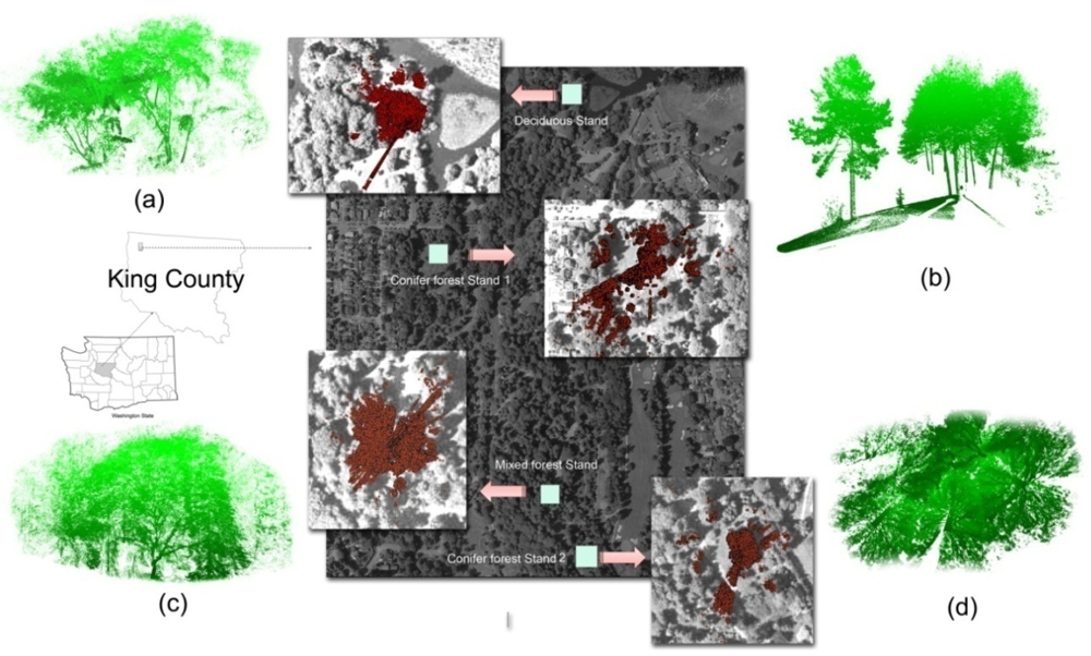
The study was conducted in the Washington Park Arboretum (WPA), located on the shores of Lake Washington, east of downtown Seattle, Washington, USA and south of the University of Washington (UW) (Figure 1). The WPA contains over 4,600 species and cultivated varieties and is one of the three most diverse collections of woody plants in the United States. Among WPA’s 20,000 trees, shrubs and vines, more than 10,000 are catalogued in collections. In this study, plots were placed in four diverse forest types, with a range of tree species including: Western redcedar (Thuja plicata), Monkey-puzzle, (Araucaria araucana), Southern magnolia (Magnolia grandiflora), Giant sequoia (Sequoiadendron giganteum), Western hemlock (Tsuga heterophylla), Oregon white oak (Quercus garryana), Douglas fir (Pseudotsuga menziesii), Vine maple (Acer circinatum), Bigleaf mape (Acer macrophyllum, Western white pine (Pinus monticola), Ponderosa pine (Pinus ponderosa), Pacific dogwood (Cornus nuttallii), and New Mexican locust (Robinia neomexicana).
2.2. Data Collection
We developed an approach to extract forest inventory parameters directly from PCD as shown in Figure 2. On September 17th through 20th, 2007, during leaf-on conditions, we used TLS to collect PCDs for four heterogeneous urban forest stands captured through four plots using a single side lateral scanning approach. Simultaneously, a stem map for each plot was generated using a Trimble surveying total station. We manually measured the DBH, basal area and tree height of each tree in all plots using tape and a TruePulse 360B Range Finder. Furthermore, each scanner location was acquired with a survey grade GPS Trimble Pro XR (Trimble Inc.) for future association with ALS data. We geo-referenced the PCD with stem map into a same projection and coordination system (GCS_North_American_1983 and Projected Coordinate System: NAD_1983_UTM_Zone_10N). In order to avoid losing PCD encompassing the tree crowns outside of the plot boundary, we created a 5 m buffer around the stem map and clipped the PCD for each plot based on our field observation; an average tree crown in our plots had a radius of 5 m, thus this value was chosen. Figure 1 shows the four plots’ PCDs, with both the scanning range and point density spatial distribution.
The tripod-mounted Leica High-Definition Surveying Systems HDS 3000™ (Leica Geosystems HDS, San Ramon, CA, USA) 3D laser scanner was used to scan the four plots. The Leica HDS 3000™ is a high-density laser scanner that emits visible green light (532 nm) laser pulses at up to 1,800 laser pulses per second. The maximum field-of-view of the scanner is 360° and 270° in the horizontal and vertical direction, respectfully. The unique dual-windows design allows for efficient utilization of its maximum field-of-view without re-orientation of the instrument, which is driven by servomotor. The spot size of HDS 3000 is 6 mm at distance of 50 m. Before starting laser scanning, we took the true color photograph for the whole field of view with the built-in integrated digital camera by automatically rotating the two internal mirrors. The imagery was used for visual interpretation of obstructions and stand characteristics to help with our results interpretation. A 2.5 cm point spacing (at 50 m) was used and scans were performed in a hemisphere commencing at the true northern direction of the sites. Because only one side lateral position was set up for scanning, some information about trees most distant from the scanner was not acquired due to occlusion [44]. We chose the side lateral scanning approach to simulate the direction a MLS instrument would collect data in an urban environment. We processed the raw PCD using Cyclone TM software version 5.8 (Leica Geosystems HDS, San Ramon, CA, USA) and converted the output into ASCII format. The 30 m by 30 m plots were extracted to do further analysis with MATLAB and C++.
2.3. Algorithm Development
2.3.1. Voxel Modeling
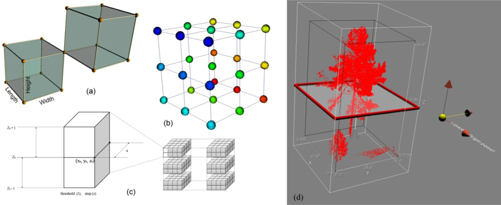
First, we selected an individual conifer tree to develop the PCS algorithm using the 3-D voxel data structure (Figure 3(a)). By defining the length, width, and height, the dimensions of each voxel were determined. We kept these consistent across the entire 3-D model space with an origin point at the laser beams exiting the scanner (Figure 3(b)). All of the coordinates of the points in real space and their corresponding coordinates in model space were denoted as (xi, yi and zi) and (x′i, y′i and z′i) respectively. The voxels constituted the 3-D model space used to reconstruct the PCD. The Z coordinates represented tree height, minimum (zmin) and maximum (zmax) from the values first calculated from the PCD. We computed the number of slice planes using the following equation (Figure 3(c)):
The length and width were denoted as the time step (s), which was the moving distance at a time of each single voxel along the axis of movement; the double threshold value, which wasthe thickness of each slice plane, determined the height of each voxel. Thus, the 3-D voxel model was set up with the threshold value (t) and time step (s), and then every point in the PCD was assigned into the corresponding slice plane by dividing the z value by the double threshold. In this way, we divided all of the points into individual slice planes. Each slice plane had a double threshold thickness, since every point coordinate in real space was converted into its corresponding coordinates in model space by calculating the ratio of x′s and y′s in the real space over the time steps (x′i = xi/s; y′i = yi/s). According to the x′i and y′i values, the points from real space were assigned to a corresponding voxel in the new model space.
2.3.2. Terrain Model for Normalizing PCD
Although various ground modeling methods have been developed for ALS [45–47], these are not easily applicable to TLS PCD due to the differences in angle of acquisition, single returns and the much higher density of the TLS data. However, methods designed for TLS have been attempted, for example, Maas, Bienert et al. [25] proposed an approach to generate TLS-based terrain model by analyzing the height histogram followed by a neighborhood consistency check and bilinear interpolation in the meshes. In this work, we developed an approach based on the voxel data structure which was similar to the method proposed by Thies, Pfeifer et al. [48]. It included two steps: first, the whole domain of the PCD for each plot was divided into finite number of equal size voxels where the height of voxel was the height of the PCD domain. Then, in each voxel, the lowest height point was found. Second, we converted the PCD into spherical coordinate system to facilitate view angle analysis based on the inclination and azimuthal angles of each point. According to the visual estimation of the maximum height of topography, the threshold of topographical variation (i.e., slope) was defined to remove the lower shrub points. Finally, we generated the triangulation and mesh for ground points to normalize the PCD to the ground.
2.4. Point Cloud Slicing (PCS)
We developed the PCS method based on the voxel data structure to retrieve forest inventory parameters from PCD generated using TLS. We sliced the PCD horizontally (Figure 3(d)) after normalizing the PCD with the terrain model. By specifying a threshold (t) and time step (s), we converted the PCD into a new voxel model space composed of hundreds of voxels. In each slice plane, the discrete points were interpolated and rasterized by coding a voxel containing at least 1 point as 1, and voxels containing no points as 0. In addition, the numbers of points within each voxel were recorded and used to indicate the point density for a voxel.
2.4.1. DBH, Basal Area, and Tree Heights Estimation
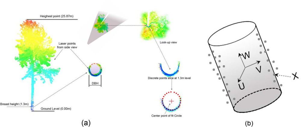
In order to extract DBH for individual trees, we sliced the PCD horizontally and extracted the point set at breast height (1.3 m). Because of occlusion (Figure 4(a)), we fitted a 3-D cylinder primitive to approximate the trunk based on the assumption that the shape of the trunk was a geometric circle. The diameter and cross-sectional area of the fitted 3-D cylinder represented the DBH and basal area for a given PCD.
The 3-D PCD S = pi (xi, yi zi) ⊂ R3 consisted of points extracted from the tree trunk surface at breast height through horizontally slicing. We fitted the 3-D PCD S using a finite cylinder with the following standard quadratic equation (Equation (4)) [49,50] as shown in Figure 4(b):
where I was the identify matrix, C was the point contained by an axis to define a finite cylinder and its unit-length direction was W. Furthermore, r was the radius of the cylinder (r > 0). The other two unit-length vectors were U and V. U, V and W were all unit-length, mutually perpendicular, which followed the right-handed orthonormal law (i.e., U × V = W, V × W = U, and W × U = V). Finally, X was any point on the cylinder, which satisfied the following condition:
where R was a rotation matrix which columns were U, V, and W, Y was a column vector which rows were y1, y2, and y3. In addition, any point X satisfied the following:
The cylinder was bounded at the axis direction by |y3| ≤ h/2(h > 0), where h was the height of the cylinder. Then we used the least-square methods to fit a cylinder primitive with a given PCD horizontally sliced from the tree trunk surface at breast height. We denoted the error distance between the actual point p and the predicted point p′ based on the Equation (4) as follows:
By minimizing the total squared error ∑i εi,we found the best parameter for Equation (4) to best fit the 3-D PCD shown in Figure 4(b). The center coordinates and DBH (i.e., diameter of cylinder) were calculated and used to represent the stem location.
The tree height information was also obtained through the horizontal PCS where the lowest and highest slice plane obtained through horizontal PCS allowed us to determine the tree height by calculating the difference between them. In addition, by using an interval space for each slice plane, stem profile information can be extracted. In turn, these measurements served as the parameters to calculate volume, and can be used in the future for aboveground biomass estimation.
2.4.2. Stem and Canopy Volume Estimation
We developed a voxel-based method to estimate above ground volume for a tree but this same approach can lead to calculations for a stand. The tree volume was obtained by summing the volumes of all voxels. One should note that in this approach the adjust factor (Vadjust) should be calculated separately for trunk volume. The following equation was used to estimate the whole tree volume from TLS:
where Vlidar was the LiDAR-based aboveground volume for a tree or a forest plot; Npts represented the numbers of points in the PCD generated from TLS for a tree or a forest plot. Moreover, Vvoxel was defined by the volume of each voxel and was calculated using height × width × length. Once the dimension of each voxel was determined, the volume for each voxel was calculated. Vadjust was the trunk volume estimated by calculating trunk volume according to the modeled DBH and tree height obtained from PCD by fitting cylinder primitive and horizontal PCS, respectively.
In this work, total volume for the forest plots was calculated using the following equation [51]:
First, the volume of each single tree was calculated based on above equation, and then the total forest plot volume (FPV) was summated by adding up all of volumes of the single trees.
3. Results
3.1. Horizontal PCS for an Individual Tree
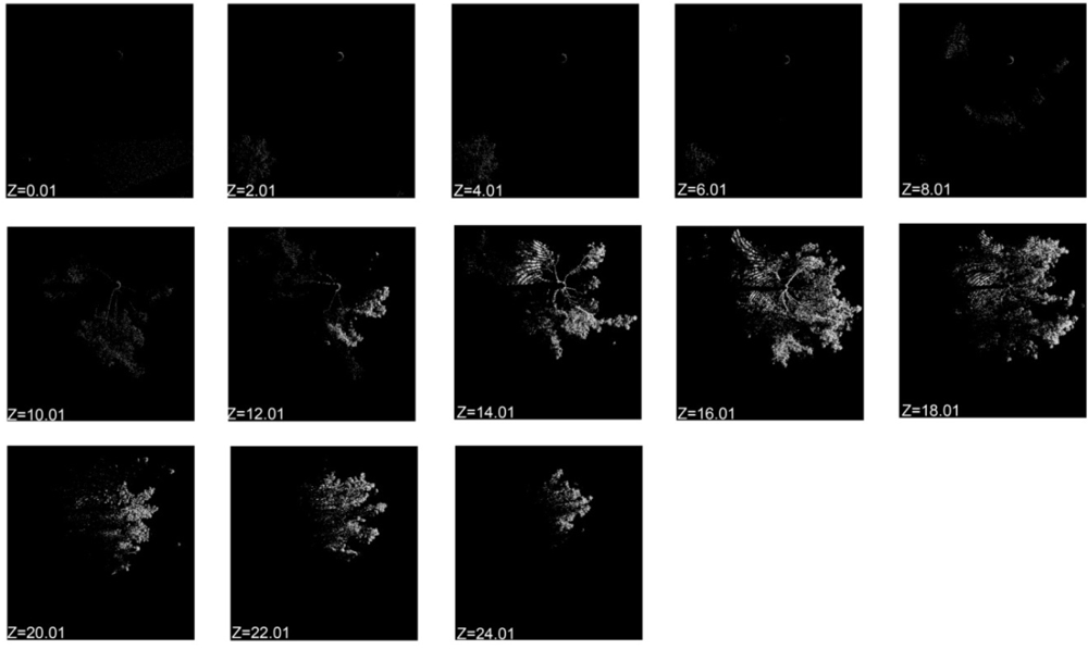
An individual conifer tree was selected to illustrate the retrieval of forest inventory parameters in Figure 5. The horizontal PCS planes provided structural information from the ground level upwards including stem center position, crown base height, and foliage element density. Figure 5 also shows spatially explicit foliage density distribution around the tree. Since all of the foliage elements within the canopy compete for resources such as water and sunlight, the multi-layer structure of the canopy which determines the spatial distribution of foliage element will not be a completely random pattern. These spatial and angular distributions of foliage elements are important for understanding the radiation regime and canopy structure per tree or at a forest stand level and should be investigated further.
3.2. DBH and Stem Location Estimation
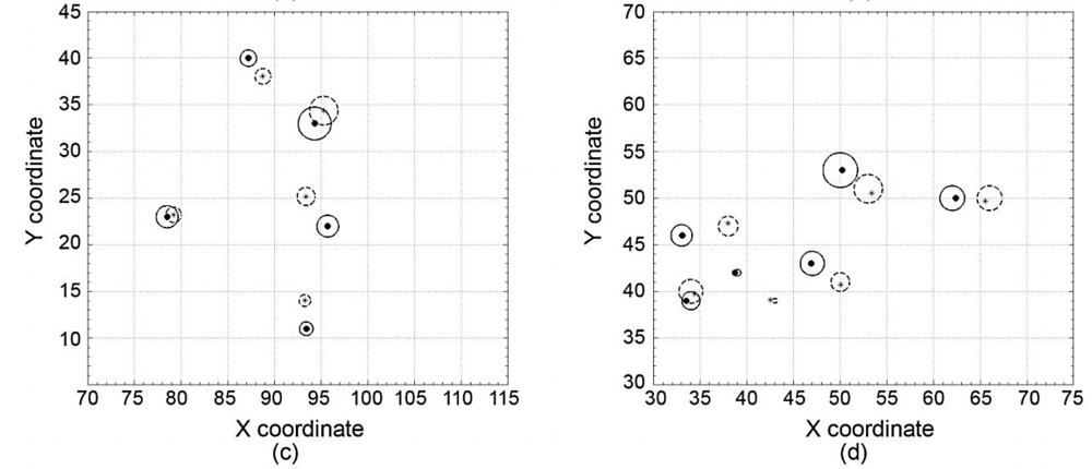
In Figure 6 we show the stem center location and DBH approximation results obtained from horizontally sliced PCD at breast height, and their comparison with the results from field measurement using the Trimble total station.
3.3. Basal Area and Tree Height Estimation
The stand basal area was calculated by summing up all the individual basal areas of the trees within a plot and results are shown in Table 1. The TBA estimated with TLS is underestimated compared to field based methods. However, since field methods generalize this measurement a more precise estimate is expected from the TLS approach, without destructive sampling it is difficult to determine the true basal area for a tree or a stand, thus, the contrast in these two methods cannot be further explained.
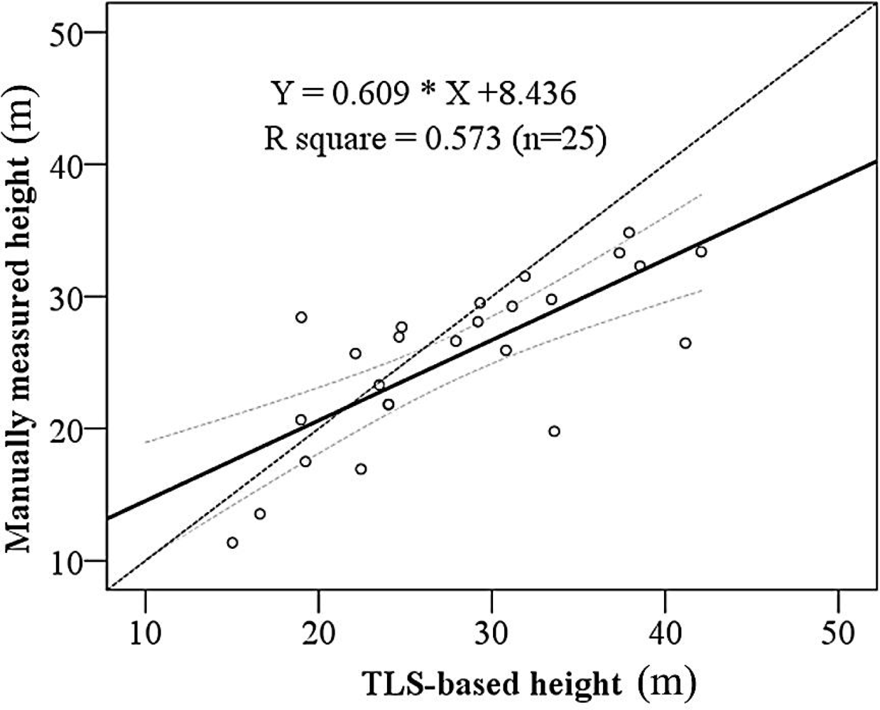
LiDAR metrics only predict 57.27% (RMSE = 0.75 m, p < 0.001) of tree height. Height analysis t-test and associated statistics of the linear models are shown in Table 2. In addition, we tested the heteroskedasticity of the two TLS based prediction models using the Breusch-Pagan (BP) test, and reported the statistics in Table 2. Our results showed that there were no heteroskedasticity issues with the data.
Similarly to basal area, underestimation results for canopy volume are found in Table 2. A separate challenge, in this case, the complexity of the tree crown, obstructed the laser beam from penetrating the canopy to reach the top of the tree. Thus, the tree height estimated with our particular terrestrial scanner was rarely the true top of individual tree or forest stand. We showed the relationship between the TLS and manually measured based height results using the validation model in Figure 7. Others have reported the same issues when attempting to use TLS for biomass estimation [52].
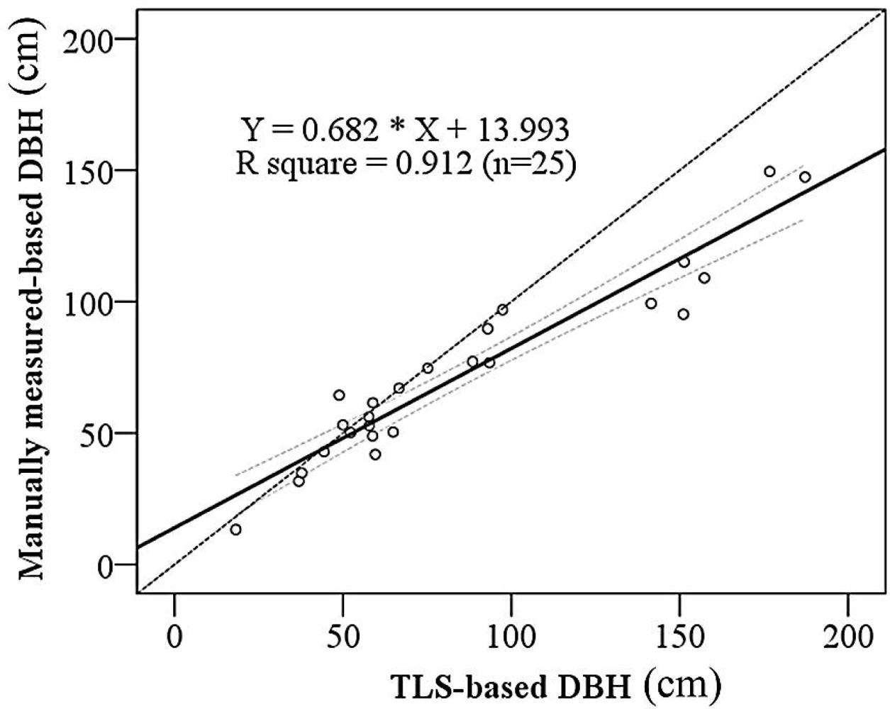
We demonstrated the correlation between the TLS-based and manually measured DBH results in Figure 8. Overall, TLS captured 91.17% (RMSE = 9.1739 cm, p < 0.001) of the variation of DBH, by visually interpreting the point cloud for stems with lowest results we conclude that occlusion is an issue, especially for large stems where parts of the stems are blocked by trees in between the stem and the scanner.
3.4. Canopy and Stem Volume Estimation
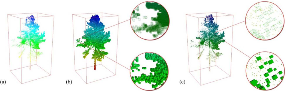
The PCD captured with TLS is a sampling technique, albeit with very high detail as show in Figure 9(a). As we mentioned above, the interval space between each point was defined before starting scanning by specifying the point-spacing parameter of scanner. The pre-defined sampling space was the most appropriate dimension parameter we suggested for the voxel-based volume estimation setting. If the size of each voxel was larger than the sampling space, it would overestimate the canopy volume. This may result in overlapping voxels (Figure 9(b)). However, if a smaller dimension is set for the voxel, it will not appropriately represent the real volume. Once the dimension of voxel has been determined by pre-defined sampling space, the whole tree volume was estimated by applying a voxel to each point (Figure 9(c)). The STV and FPV estimating results were presented in the Table 4. TLS tends to underestimate these values compared to our field method; this is especially true for very large conifers in the conifer-2 stand. The voxel-based tree canopy volume estimation shows potential to solve the issue of overestimation of tree canopy volume resulting from the tree wrapping method [42], and the crown geometric volume method [52], since the method does not include the gaps between the foliage elements within tree canopy in the total volume estimate.
4. Discussion
Although the results obtained from voxel-based PCS method showed good agreement with the field measurements, some factors still influence the accuracy. For example, we show that in heterogeneous forests, such as those in an urban setting, instrument setup is critical for the purpose of occlusion reduction which can improve accuracies; others have shown this in non-urban environments [31,53]. The occlusion could be offset or improved by setting up two or more vantage points to scan the same tree or plot [54]. However, the two or more PCDs must be co-registered before further processing, thus, complicating and extending the time of the field campaign. This is in agreement with the findings by Watt and Donoghue [31].
To slice the PCD using the 3-D voxel approach one needs to control the step (s) and threshold (t) of the voxelization parameters. These should be adjusted according to specific application. However these parameters can be impacted and potentially limited by point spacing of the scanner. For example, for the Leica HDS 3000, the minimum point spacing can be set to 0.001 m at the finest setting. Thus, when specifying these parameters, three sides should be provided to determine the dimensions of the 3-D voxels; the parameter step (s) will control two sides of bottom square, and threshold (t) will determine the height of each voxel. In this work, for individual trees, the step (s) was assigned 0.01 m and threshold was assigned 2 m. However, for the forest stand PCD, the amount of total points will greatly increase, and we recommend raising the step (s) settings up to 0.4 m to increase processing efficiency. These values are sufficient for normal forest inventory extraction in heterogeneous forests.
Four forest type stands were investigated in this work. The stems were relatively straight for coniferous tree, thus, the cylinder approximation works very well in this case. However, in the case of deciduous tree, the trunk and branches were so contorted that a cylinder model is not the best way to approximate tree volumes. Further research into better trunk representation models is needed. In addition, the crown base height of the canopy will significantly affect the accuracy of stem location map, due to visibility and leaning. By using horizontal slicing, the PCD extracted at breast height was separated from the other stems; it would be more accurate to approximate the cylinder (3D) to reconstruct the DBH and basal area.
We show that the tree age and size greatly affect the accuracy of TLS-based metrics, especially DBH. This finding is consistent with Murphy’s [35] results. Moreover, the bigger the tree size, the more severe the occlusion effect. For example, conifer 2 plot dominated by mature forest trees including a Giant Sequoia (Sequoiadendron giganteum) aged over 60 years, showed such severe occlusion it lead us to conclude that the single-lateral scanning approach was not capable of capturing a representative PCD for this type of a complex forest stands. This finding has implications for applying MLS or VLS to forest inventories in urban areas and to rapid biomass estimation at individual tree level [52,54,55], moreover it suggests that sampling strategies need to be further investigated along the lines pioneered by Pesci et al. [56].
5. Conclusions
In this work, we introduced a voxel-based point cloud slicing (PCS) method to post-process point cloud data (PCD) obtained from terrestrial laser scanning (TLS) leading to the extraction of forest inventory parameters including not only the conventional parameters such as diameter at breast height (DBH), but also tree canopy volume and basal area. Our results showed an approach to extract forest inventory parameters directly from PCD generated by TLS at forest plot and individual tree level. Thus, an opportunity exists to use TLS as a tool for calibration of ALS-derived forest inventories, biomass estimation and canopy assessments. Our results showed that PCD generated from TLS single location scans only captures 18% of the total tree volume due to an occlusion effect; yet there are significant relationships between other forest inventory data captured by the TLS giving promise to the utility of a side scanning approach. We do recommend that alternative TLS scanning locations should be combined with the single side-lateral scan to improve volume and biomass estimation by reducing occlusion. Presently, it is still not feasible to use TLS as an operational field tool due to weight, scanning speed and instrument costs. But even with its limitations, it has been suggested that TLS is the only comprehensive, repeatable and non-destructive way to characterize forest stands for biomass estimation. Moreover, in the last 5 years, exceptional strides have been made by the industry to increase the speed of the scanners, reduce their size and improve portability, pricing has also dropped. These, combined with stereoscopic field photography and open-source tools that allow for PCD generation from photography, as well as MLS, are providing datasets ideal for our PCS method. As tools for PCD analysis are being developed, we need parallel efforts to determine robust techniques for sampling strategies and protocols utilizing TLS and tools for optimizing and combining these data in conjunction with other inventory techniques.
Acknowledgments
We conducted this research at the University of Washington Remote Sensing and Geospatial Analysis Laboratory (UW RSGAL) and International Institute for Earth System Science, Nanjing University. Funding and resources for this research project came from the NSF funded University of Washington I/UCRC Center for Advanced Forest Systems (NSF award # 0855690), the state key fundamental science funds of China (2010CB950701), the open research fund program of State Key Laboratory of Hydroscience and Engineering in Tsinghua University (sklhse-2012-B-04) and the University of Washington Precision Forestry Cooperative. We acknowledge our field assistants: Jeffery Richardson, Akira Kato, Michael Hannam and Nicole Hackman for help with the TLS data acquisition. Finally, we thank the three anonymous reviewers who helped us improve this manuscript.
References
- Fernandes, P.M. Combining forest structure data and fuel modelling to classify fire hazard in Portugal. Ann. For. Sci 2009, 66. [Google Scholar] [CrossRef]
- Zheng, G.; Chen, J.M.; Tian, Q.; Ju, W.M.; Xia, X.Q. Combining remote sensing imagery and forest age inventory for biomass mapping. J. Environ. Manage 2007, 85, 616–623. [Google Scholar]
- Wang, B.; Huang, J.Y.; Yang, X.S.; Zhang, B.A.; Liu, M.C. Estimation of biomass, net primary production and net ecosystem production of China’s forests based on the 1999–2003 national forest inventory. Scand. J. For. Res 2010, 25, 544–553. [Google Scholar]
- Van Deusen, P. Carbon sequestration potential of forest land: Management for products and bioenergy versus preservation. Biomass Bioenergy 2010, 34, 1687–1694. [Google Scholar]
- Thony, P.; Mabee, W.; Kozak, R.; Bull, G. A characterization of the british columbia log home and timber frame manufacturing sector. Forest. Chron 2006, 82, 77–83. [Google Scholar]
- Cottone, N.; Ettl, G.J. Estimating populations of whitebark pine in mount rainier national park, washington, using aerial photography. Northwest Sci 2001, 75, 397–406. [Google Scholar]
- Barclay, H.J.; Li, C.; Benson, L.; Taylor, S.; Shore, T. Effects of fire return rates on traversability of lodgepole pine forests for mountain pine beetle (coleoptera:Scolytidae) and the use of patch metrics to estimate traversability. Can. Entomol 2005, 137, 566–583. [Google Scholar]
- Pothier, D. Twenty-year results of precommercial thinning in a balsam fir stand. Forest Ecol. Manage 2002, 168, 177–186. [Google Scholar]
- Patenaude, G.; Milne, R.; Dawson, T.P. Synthesis of remote sensing approaches for forest carbon estimation: Reporting to the Kyoto Protocol. Environ. Sci. Policy 2005, 8, 161–178. [Google Scholar]
- Kim, Y.; Yang, Z.Q.; Cohen, W.B.; Pflugmacher, D.; Lauver, C.L.; Vankat, J.L. Distinguishing between live and dead standing tree biomass on the north rim of Grand Canyon National Park, USA using small-footprint lidar data. Remote Sens. Environ 2009, 113, 2499–2510. [Google Scholar]
- Chen, J.M.; Chen, X.Y.; Ju, W.M.; Geng, X.Y. Distributed hydrological model for mapping evapotranspiration using remote sensing inputs. J. Hydrol 2005, 305, 15–39. [Google Scholar]
- Nikolov, N.; Zeller, K.F. Modeling coupled interactions of carbon, water, and ozone exchange between terrestrial ecosystems and the atmosphere. I: Model description. Environ. Pollut 2003, 124, 231–246. [Google Scholar]
- Richardson, J.J.; Moskal, L.M.; Kim, S.H. Modeling approaches to estimate effective leaf area index from aerial discrete-return lidar. Agric. Forest Meteorol 2009, 149, 1152–1160. [Google Scholar]
- Moskal, L.M.; Styers, D.M.; Halabisky, M. Monitoring urban tree cover using object-based image analysis and public domain remotely sensed data. Remote Sens 2011, 3, 2243–2262. [Google Scholar]
- Henning, J.G.; Radtke, P.J. Ground-based laser imaging for assessing three-dimensional forest canopy structure. Photogramm. Eng. Remote Sensing 2006, 72, 1349–1358. [Google Scholar]
- Niinemets, U. Photosynthesis and resource distribution through plant canopies. Plant Cell Environ 2007, 30, 1052–1071. [Google Scholar]
- Utsugi, H.; Araki, M.; Kawasaki, T.; Ishizuka, M. Vertical distributions of leaf area and inclination angle, and their relationship in a 46-year-old chamaecyparis obtusa stand. Forest Ecol. Manage 2006, 225, 104–112. [Google Scholar]
- Li, F.S.; Cohen, S.; Naor, A.; Kang, S.Z.; Erez, A. Studies of canopy structure and water use of apple trees on three rootstocks. Agric. Water Manage 2002, 55, 1–14. [Google Scholar]
- Macfarlane, C.; Grigg, A.; Evangelista, C. Estimating forest leaf area using cover and fullframe fisheye photography: Thinking inside the circle. Agric. Forest Meteorol 2007, 146, 1–12. [Google Scholar]
- Zhang, S.Y.; Lei, Y.C.; Bowling, C. Quantifying stem quality characteristics in relation to initial spacing and modeling their relationship with tree characteristics in black spruce (picea mariana). Northern J. Appl. Forest 2005, 22, 85–93. [Google Scholar]
- Evans, D.L.; Roberts, S.D.; Parker, R.C. Lidar—A new tool for forest measurements? Forest Chron 2006, 82, 211–218. [Google Scholar]
- van Leeuwen, M.; Nieuwenhuis, M. Retrieval of forest structural parameters using lidar remote sensing. Eur. J. For. Res 2010, 129, 749–770. [Google Scholar]
- Jang, J.D.; Payan, V.; Viau, A.A.; Devost, A. The use of airborne lidar for orchard tree inventory. Int. J. Remote Sens 2008, 29, 1767–1780. [Google Scholar]
- Naesset, E. Airborne laser scanning as a method in operational forest inventory: Status of accuracy assessments accomplished in Scandinavia. Scand. J. Forest Res 2007, 22, 433–442. [Google Scholar]
- Maas, H.G.; Bienert, A.; Scheller, S.; Keane, E. Automatic forest inventory parameter determination from terrestrial laser scanner data. Int. J. Remote Sens 2008, 29, 1579–1593. [Google Scholar]
- Erdody, T.L.; Moskal, L.M. Fusion of lidar and imagery for estimating forest canopy fuels. Remote Sens. Environ 2010, 114, 725–737. [Google Scholar]
- Anderson, J.E.; Plourde, L.C.; Martin, M.E.; Braswell, B.H.; Smith, M.L.; Dubayah, R.O.; Hofton, M.A.; Blair, J.B. Integrating waveform lidar with hyperspectral imagery for inventory of a northern temperate forest. Remote Sens. Environ 2008, 112, 1856–1870. [Google Scholar]
- Hyyppa, J.; Hyyppa, H.; Leckie, D.; Gougeon, F.; Yu, X.; Maltamo, M. Review of methods of small-footprint airborne laser scanning for extracting forest inventory data in boreal forests. Int. J. Remote Sens 2008, 29, 1339–1366. [Google Scholar]
- Hill, R.A.; Thomson, A.G. Mapping woodland species composition and structure using airborne spectral and lidar data. Int. J. Remote Sens 2005, 26, 3763–3779. [Google Scholar]
- Vaughn, N.R.; Moskal, L.M.; Turnblom, E.C. Fourier transformation of waveform lidar for species recognition. Remote Sens. Lett 2011, 2, 347–356. [Google Scholar]
- Watt, P.J.; Donoghue, D.N.M. Measuring forest structure with terrestrial laser scanning. Int. J. Remote Sens 2005, 26, 1437–1446. [Google Scholar]
- Tansey, K.; Selmes, N.; Anstee, A.; Tate, N.J.; Denniss, A. Estimating tree and stand variables in a corsican pine woodland from terrestrial laser scanner data. Int. J. Remote Sens 2009, 30, 5195–5209. [Google Scholar]
- Lovell, J.L.; Jupp, D.L.B.; Newnham, G.J.; Culvenor, D.S. Measuring tree stem diameters using intensity profiles from ground-based scanning lidar from a fixed viewpoint. ISPRS J. Photogramm 2011, 66, 46–55. [Google Scholar]
- Huang, H.B.; Li, Z.; Gong, P.; Cheng, X.A.; Clinton, N.; Cao, C.X.; Ni, W.J.; Wang, L. Automated methods for measuring DBH and tree heights with a commercial scanning lidar. Photogramm. Eng. Remote Sensing 2011, 77, 219–227. [Google Scholar]
- Murphy, G. Determining stand value and log product yields using terrestrial lidar and optimal bucking: A case study. J. Forest 2008, 106, 317–324. [Google Scholar]
- Omasa, K.; Urano, Y.; Oguma, H.; Fujinuma, Y. Mapping of tree position of larix leptolepis woods and estimation of diameter at breast height (DBH) and biomass of the trees using range data measured by a portable scanning lidar. J. Remote Sens. Soc. Jpn 2002, 22, 550–557. [Google Scholar]
- Hopkinson, C.; Chasmer, L. Testing lidar models of fractional cover across multiple forest ecozones. Remote Sens. Environ 2009, 113, 275–288. [Google Scholar]
- Weiss, J. Application and statistical analysis of terrestrial laser scanning and forest growth simulations to determine selected characteristics of douglas-fir stands. Felia Forestalia Polonica 2009, 51, 123–137. [Google Scholar]
- Yao, T.; Yang, X.; Zhao, F.; Wang, Z.; Zhang, Q.; Jupp, D.; Lovell, J.; Culvenor, D.; Newnham, G.; Ni-Meister, W.; et al. Measuring forest structure and biomass in New England forest stands using echidna ground-based lidar. Remote Sens. Environ 2011, 115, 2965–2974. [Google Scholar]
- Popescu, S.C. Estimating biomass of individual pine trees using airborne lidar. Biomass Bioenergy 2007, 31, 646–655. [Google Scholar]
- Jupp, D.L.B.; Culvenor, D.S.; Lovell, J.L.; Newnham, G.J.; Strahler, A.H.; Woodcock, C.E. Estimating forest lai profiles and structural parameters using a ground-based laser called “echidna (r)”. Tree Physiol 2009, 29, 171–181. [Google Scholar]
- Kato, A.; Moskal, L.M.; Schiess, P.; Swanson, M.E.; Calhoun, D.; Stuetzle, W. Capturing tree crown formation through implicit surface reconstruction using airborne lidar data. Remote Sens. Environ 2009, 113, 1148–1162. [Google Scholar]
- van Aardt, J.A.N.; Wynne, R.H.; Scrivani, J.A. Lidar-based mapping of forest volume and biomass by taxonomic group using structurally homogenous segments. Photogramm. Eng. Remote Sensing 2008, 74, 1033–1044. [Google Scholar]
- Zheng, G.; Moskal, L.M. Retrieving leaf area index (LAI) using remote sensing: Theories, methods and sensors. Sensors 2009, 9, 2719–2745. [Google Scholar]
- Chen, Q.; Gong, P.; Baldocchi, D.; Xie, G. Filtering airborne laser scanning data with morphological methods. Photogramm. Eng. Remote Sensing 2007, 73, 175–185. [Google Scholar]
- Kraus, K.; Pfeifer, N. Determination of terrain models in wooded areas with airborne laser scanner data. ISPRS J. Photogramm 1998, 53, 193–203. [Google Scholar]
- Kobler, A.; Pfeifer, N.; Ogrinc, P.; Todorovski, L.; Ostir, K.; Dzeroski, S. Repetitive interpolation: A robust algorithm for dtm generation from aerial laser scanner data in forested terrain. Remote Sens. Environ 2007, 108, 9–23. [Google Scholar]
- Thies, M.; Pfeifer, N.; Winterhalder, D.; Gorte, B.G.H. Three-dimensional reconstruction of stems for assessment of taper, sweep and lean based on laser scanning of standing trees. Scand. J. Forest Res 2004, 19, 571–581. [Google Scholar]
- Schneider, P.J.; Eberly, D.H. Appendix A: Numerical methods. In Geometric Tools for Computer Graphics; Morgan Kaufmann Publishers: Amsterdam, The Netherlands, 2003; pp. 882–889. [Google Scholar]
- Eberly, D. Fitting 3D Data with a Cylinder; Geometric Tools, LLC.: Scottsdale, AZ, USA, 2008. Available online: http://www.geometrictools.com/Documentation/CylinderFitting.pdf (accessed on 5 February 2011).
- Bouriaud, O.; Soudani, K.; Breda, N. Leaf area index from litter collection: Impact of specific leaf area variability within a beech stand. Can. J. Remote Sens 2003, 29, 371–380. [Google Scholar]
- Jung, S.-E.; Kwak, D.-A.; Park, T.; Lee, W.-K.; Yoo, S. Estimating crown variables of individual trees using airborne and terrestrial laser scanners. Remote Sens 2011, 3, 2346–2363. [Google Scholar]
- Lin, Y.; Jaakkola, A.; Hyyppä, J.; Kaartinen, H. From TLS to VLS: Biomass estimation at individual tree level. Remote Sens 2010, 2, 1864–1879. [Google Scholar]
- Van der Zande, D.; Hoet, W.; Jonckheere, I.; van Aardt, J.; Coppin, P. Influence of measurement set-up of ground-based lidar for derivation of tree structure. Agric. Forest. Meteorol 2006, 141, 147–160. [Google Scholar]
- Seielstad, C.; Stonesifer, C.; Rowell, E.; Queen, L. Deriving fuel mass by size class in Douglas-fir (Pseudotsuga menziesii) using terrestrial laser scanning. Remote Sens 2011, 3, 1691–1709. [Google Scholar]
- Pesci, A.; Teza, G.; Bonali, E. Terrestrial laser scanner resolution: Numerical simulations and experiments on spatial sampling optimization. Remote Sens 2011, 3, 167–184. [Google Scholar]
Figure 1.
Study area and point clouds for four forest types: (a) deciduous forest stand; (b) conifer-1 forest stand; (c) mixed forest stand; (d) conifer-2 forest stand. The background picture is a panchromatic aerial photo of Washington Park Arboretum overlaid with corresponding point cloud data (red dots). The 3-D perspective view of point cloud data (green points) are shown next to each plot.

Figure 2.
Flowchart of forest inventory parameters estimation from TLS. The dash line box represents the TLS-based forest inventory parameters which were compared with field-based manual measurements.
Figure 2.
Flowchart of forest inventory parameters estimation from TLS. The dash line box represents the TLS-based forest inventory parameters which were compared with field-based manual measurements.
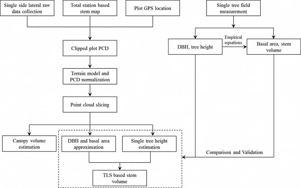
Figure 3.
Dimensional information for each voxel is shown in (a); the voxel data structure (2 × 2 × 2) visualization is shown in (b); the schematic diagram for the PCS is shown in (c); and, the voxel-based PCS plane for an individual tree PCD is shown in (d).
Figure 3.
Dimensional information for each voxel is shown in (a); the voxel data structure (2 × 2 × 2) visualization is shown in (b); the schematic diagram for the PCS is shown in (c); and, the voxel-based PCS plane for an individual tree PCD is shown in (d).

Figure 4.
Schematic diagram of occlusion is shown in (a), and 3-D cylinder primitive fitting technique is shown in (b).
Figure 4.
Schematic diagram of occlusion is shown in (a), and 3-D cylinder primitive fitting technique is shown in (b).

Figure 5.
Thirteen horizontal slice planes for individual tree PCD at a 2 m distance interval with 0.01 steps (Z values represent the height of each slice plane at meters unit).
Figure 5.
Thirteen horizontal slice planes for individual tree PCD at a 2 m distance interval with 0.01 steps (Z values represent the height of each slice plane at meters unit).

Figure 6.
Comparison between measured and modeled stem location and DBH approximations for four forest stands: (a) conifer-2 forest stand; (b) conifer-1 forest stand; (c) deciduous forest stand; and (d) mixed forest stand. Solid circles represent the measured stem location, star symbols represent modeled stem location, solid line circles represent measured DBH approximation, and the dashed line circles represent modeled DBH approximation.
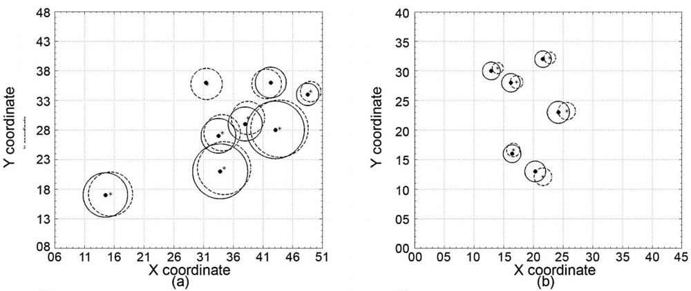

Figure 7.
Comparison between measured and modeled height (in m) using PCS; solid line is a prediction model for TLS- based height (N = 25, RMSE = 0.75 m, p < 0.001).
Figure 7.
Comparison between measured and modeled height (in m) using PCS; solid line is a prediction model for TLS- based height (N = 25, RMSE = 0.75 m, p < 0.001).

Figure 8.
Comparison between measured and modeled DBH (in cm) using the PCS for the four forest stands; the solid line is a linear prediction model for TLS-based DBH (N = 25, RMSE = 9.1739 cm, p < 0.001).
Figure 8.
Comparison between measured and modeled DBH (in cm) using the PCS for the four forest stands; the solid line is a linear prediction model for TLS-based DBH (N = 25, RMSE = 9.1739 cm, p < 0.001).

Figure 9.
Schematic diagram for canopy volume estimation from TLS where: (a) is the raw PCD visualization result with bounding box; (b) is the voxel-based canopy volume visualization results with 10 times amplification of sampling spacing for each voxel size; and, (c) is the voxel-based canopy volume visualization results with the sampling spacing voxel size. In (b) and (c) the wireframe (top) and surface representation forms of voxels are shown as well.


| Conifer-1 | Conifer-2 | Deciduous | Mixed | |||||
|---|---|---|---|---|---|---|---|---|
| Field-TBA | TLS-TBA | Field-TBA | TLS-TBA | Field-TBA | TLS-TBA | Field-TBA | TLS-TBA | |
| 0.1122 | 0.0951 | 1.7979 | 1.0405 | 0.279 | 0.1379 | 0.6866 | 0.4632 | |
| 0.2148 | 0.1979 | 2.4522 | 1.7554 | 0.1548 | 0.1445 | 0.3308 | 0.1995 | |
| — | 0.2215 | 2.7523 | 1.7064 | 0.6151 | 0.4681 | 0.2624 | 0.219 | |
| 0.2615 | 0.2481 | 1.9433 | 0.9331 | 0.2715 | 0.1878 | 0.3494 | 0.3536 | |
| 0.7451 | 0.7375 | 1.7932 | 0.7118 | 0.1069 | 0.0789 | 0.026 | 0.0139 | |
| 0.6793 | 0.6319 | 1.5725 | 0.7744 | 0.1878 | 0.3257 | |||
| 0.2725 | 0.2971 | |||||||
| 0.4441 | 0.4383 | |||||||
| SBAA | 2.7295 | 2.8673 | 12.3116 | 6.9217 | 1.4275 | 1.0172 | 1.8431 | 1.575 |
| Coefficient | Estimate | Standard Error | t-Value | P-Value | |
|---|---|---|---|---|---|
| DBH-prediction | Intercept | 13.993 | 4.299 | 3.255 | 0.003 |
| Manually measured-based DBH | 0.682 | 0.044 | 15.407 | 0.000 | |
| Height-prediction | Intercept | 8.436 | 3.177 | 2.656 | 0.014 |
| TLS-based tree height | 0.609 | 0.110 | 5.552 | 0.000 | |
| BP Value | Degree of Freedom | P-Value | Chi-Square Value (95% level) | |
|---|---|---|---|---|
| TLS-DBH prediction | 1.725 | 1 | 0.189 | 3.841 |
| TLS-height prediction | 0.293 | 1 | 0.585 | 3.841 |
| Conifer-1 | Conifer-2 | Deciduous | Mixed | |||||
|---|---|---|---|---|---|---|---|---|
| Field-STV | TLS-STV | Field-STV | TLS-STV | Field-STV | TLS-STV | Field--STV | TLS-STV | |
| 0.88 | 0.74 | 22.73 | 13.15 | 4.40 | 2.97 | 2.23 | 1.10 | |
| — | 1.69 | 26.08 | 18.67 | 3.22 | 1.94 | 0.78 | 0.72 | |
| 1.58 | 1.53 | 35.37 | 21.93 | 2.94 | 2.45 | 4.93 | 3.75 | |
| 2.43 | 2.20 | 24.20 | 11.62 | 3.42 | 3.46 | 2.03 | 1.40 | |
| 7.65 | 6.37 | 24.61 | 9.77 | 0.16 | 0.09 | 0.59 | 0.44 | |
| 7.06 | 6.16 | 22.06 | 10.86 | 1.55 | 2.69 | |||
| 3.04 | 2.95 | |||||||
| 3.65 | 3.94 | |||||||
| FPV t | 21.40 | 25.58+0.0045 | 155.06 | 86.01+0.0038 | 15.69 | 13.60+0.0017 | 10.56 | 7.42+0.0037 |
Share and Cite
MDPI and ACS Style
Moskal, L.M.; Zheng, G. Retrieving Forest Inventory Variables with Terrestrial Laser Scanning (TLS) in Urban Heterogeneous Forest. Remote Sens. 2012, 4, 1-20. https://doi.org/10.3390/rs4010001
AMA Style
Moskal LM, Zheng G. Retrieving Forest Inventory Variables with Terrestrial Laser Scanning (TLS) in Urban Heterogeneous Forest. Remote Sensing. 2012; 4(1):1-20. https://doi.org/10.3390/rs4010001
Chicago/Turabian StyleMoskal, L. Monika, and Guang Zheng. 2012. "Retrieving Forest Inventory Variables with Terrestrial Laser Scanning (TLS) in Urban Heterogeneous Forest" Remote Sensing 4, no. 1: 1-20. https://doi.org/10.3390/rs4010001