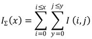
Article

Automatic Registration of Airborne and Spaceborne Images by Topology Map Matching with SURF Processor Algorithm

Remote Sensing Laboratory, Department of Geography and Human Environment, Tel-Aviv University, Ramat Aviv, P.O. Box 39040, Tel Aviv 69978, Israel
*
Author to whom correspondence should be addressed.
Remote Sens. 2011, 3(1), 65-82; https://doi.org/10.3390/rs3010065
Submission received: 16 November 2010 / Revised: 24 December 2010 / Accepted: 4 January 2011 / Published: 6 January 2011
(This article belongs to the Special Issue 100 Years ISPRS - Advancing Remote Sensing Science)

Abstract

:
Image registration is widely used in remote-sensing applications. The existing automatic image registration techniques fall into two categories: Intensity-based and feature-based; the latter (which extracts structures from both images) being more suitable for multi-sensor fusion, detection of temporal changes and image mosaicking. Conventional image registration algorithms have proven to be inaccurate, time-consuming, and unfeasible due to image complexity which makes it cumbersome or even impossible to discern the appropriate control points. In this study, we propose a novel method for automatic image registration based on topology (AIRTop) for change detection and multi‑sensor (airborne and spaceborne) fusion. In this algorithm, we first apply image‑processing methods (SURF—Speeded-Up Robust Features) to extract the landmark structures (roads and buildings) and convert them to a features (vector) map. The following stages are applied in GIS (Geographic Information System), where topology rules, which define the permissible spatial relationships between features, are defined. The relationships between features are established by weight-based topological map-matching algorithm (tMM). The suggested algorithm presents a robust method for image registration. The main focus in this study is on scale and image rotation, when the quality of the scanning system is constant. These seem to offer a good compromise between feature complexity and robustness to commonly occurring deformations. The skew and the anisotropic scaling are assumed to be second-order effects that are covered to some degree by the overall robustness of the sensor.

1. Introduction

Image registration is a critical pre-processing procedure in all remote-sensing applications that utilizes multiple image inputs, including multi-sensor image fusion, temporal change detection, and image mosaicking. The recent interest in change detection and modeling has brought automatic image registration into the limelight [1].
In manual registration, the selection of control points (CPs) is usually performed by a human operator. This has proven to be inaccurate, time-consuming, and unfeasible due to image complexity, which makes it cumbersome or even impossible for the human eye to discern the suitable CPs. Therefore, researchers focused on automating feature detection to align two or more images with no need for human intervention. The automatic registration of images has generated extensive research interest in the fields of computer vision, medical imaging and remote sensing. Comprehensive reviews have been published by Brown [2] and Zitova and Flusser [3].
Many proposed schemes for automatic registration employ a multi-resolution process. The discrete wavelet transform (DWT) is employed to register satellite images [4], and the modulus maxima are applied to the LH and HL frequency bands in order to extract edge points; correlation is then applied for matching. Le Moigne et al. [1] developed a parallel algorithm using the maxima of DWT coefficients for the feature space, and correlation for the search space. Mutual information (MI) methods, originating with Viola and Wells [5], are able to register multimodal images since MI represents a measure of statistical dependency between the reference and the sensed images rather than gray intensity values, which vary when different types of imagers are used, or under different lighting conditions. Registration of a multimodal brain image [6,7,8,9,10] combines the sum of the difference (SAD) and MI into a matching criterion to enhance registration accuracy. Even though the SAD is applied directly to the gray intensity values, the authors claim that their algorithm works for multimodal images.
The existing automatic image-registration techniques that are based on spatial information fall into two categories: Intensity-based and feature-based [3]. The feature-based technique extracts salient structures from sensed and reference images by accurate feature detector and by the overlap criterion. As the significant regions (e.g., roofs) considered, and lines (e.g., roads), are expected to be stable in time at a fixed position, the feature-based method is more suitable for multi-sensor fusion, change detection and image mosaicking. The method generally consists of four steps [12]: (1) CP extraction; (2) transformation-model determination; (3) image transformation and resampling; and (4) assessment of registration accuracy. The first step is the most complex, and its success essentially determines registration accuracy. Thus, the detection method should be able to detect the same features in all projections and at different radiometrical sensitivities regardless of the particular image/sensor deformation. Despite the achieved performance, the existing methods operate directly on gray intensity values and hence they are not suited for handling multi-sensor images.
The search for discrete CPs can be divided into three main steps: (1) Selection of “interesting points”; (2) description of nearest points or features; (3) matching between images. The most valued property of CP detection is its repeatability. The description of nearest points has to be distinctive but robust to noise, and potential displacements such as geometric and radiometric deformations. To succeed, the matching technique has to be accurate and sufficient while the detection scheme has to simplify the above requirements. This paper presents a novel method for automatic image registration based on topology rules (AIRTop) for change detection and multi-sensor (airborne and spaceborne) fusion.

2. Automatic Image Registration

The AIRTop algorithm (Figure 1) consists of the four stages of any conventional registration method. First, the significant features are extracted by applying SURF (Speeded-Up Robust Features) method [13] on both sensed and reference images and converted to vector format. The spatial distribution and relationship of these features is expressed by topology rules and converts them to potential CPs by determining a transformation model between sensed and reference images. The defined rules for a weight-based topological map-matching (tMM) algorithm manage [14], transform and resample features of the sensed image according to a reference image.
Since AIRTop has a sufficient number of CPs, the registration accuracy can be estimated by test point error (TPE) technique [15]. The results of the map-matching are determined by predefined Root Mean Square Error (RMSE) threshold. If the algorithm fails to identify the correct CPs among the candidate features, then the algorithm regenerates another set of random values of coefficients and repeats the map-matching. This process continues by optional loop procedure until the algorithm selects the correct CPs.
The threshold decision for a map-matching procedure is similar to the automatic segmentation problem where scale of values can be used for classification. In general, the threshold is placed at the minimum value of the histogram. We employ a statistical approach based upon a parameter model that fits the sum of the functions to the normally distributed histogram. The squared means of the normally distributed quantities of each algorithm’s stage could be modeled as a noncentral chi-squared distribution (having zero degree of freedom) [10]. We suggest automatizing selection of thresholds by calculating the power of test (using ncx2stat function, MATLAB 2009b) on the mean of a normal distribution. Thus, we achieve the regulation of the threshold.
Figure 1. A flow-chart describing the AIRTop algorithm. Red box is stage 1 (feature extraction), blue box is stage 2 (topology map matching), orange box is stage 3 (matching process), green box is stage 4 (validation and accuracy).
Remotesensing 03 00065 g001

2.1. Significant Features

CP identification is the key step in image registration. There are two main methods to detect CPs: area-based and feature-based. In feature-based algorithms, an image is represented in a compact form by a set of features. The common features are edges, regions, lines, line endings, line intersections, or region centroids. Thus, the feature-based methods are adopted when objects’ features are distinct. These methods are relatively more powerful for the registration of different types of images with distortions.
Because the image scenes studied in this research have a large area, region of interest (ROI) selection, which contains relatively large radiometric variation (grayscale contrasts), is conducted prior to feature detection. The idea of addressing the registration problem by applying a global-to-local level strategy has proven to be an elegant way of speeding up the whole process, while enhancing the accuracy of the registration procedure [11]. Thus, we expected this method to greatly reduce false alarms in the subsequent feature extraction and CP identification steps. To select the distinct areas, an image is divided into adjacent small blocks (10% × 10% of image pixels with no overlap between blocks). Then, entropy is calculated for each block (with a filter size of 20% × 20% of the pixel block), which can be used to measure the local variation within the block. 
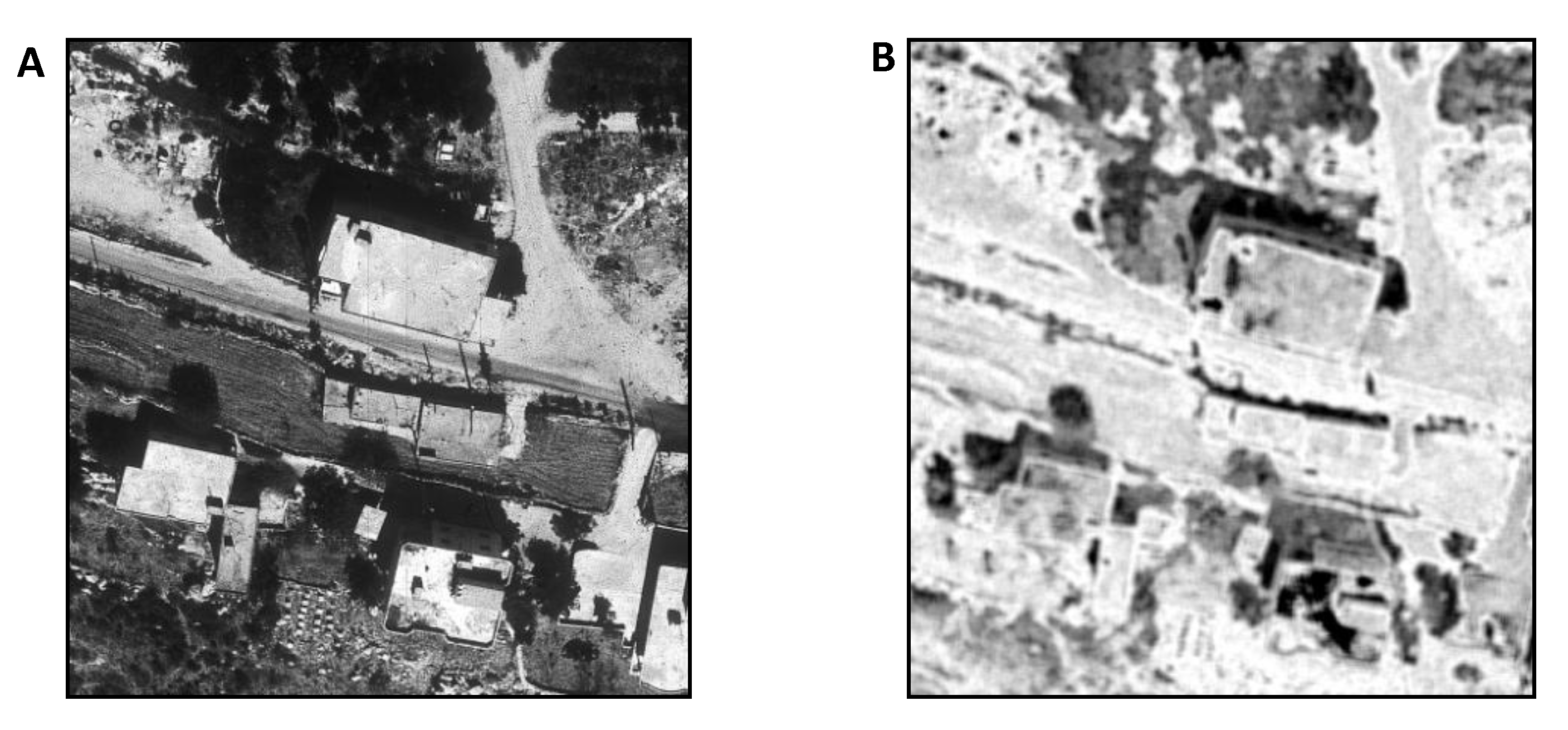
Figure 2 shows the entropy map of an image (subset of one block) of 420 × 420 pixels, where the blocks with large entropies correspond to the areas with relatively high variation, such as buildings (two roofs in the center of the image) and roads (located in the upper right part of the image). A threshold η is set to choose the blocks with large entropies as ROIs for CP detection. This ensures that at least one ROI will be selected from each patch, which may result in a wider distribution of CPs.
Significant features are then extracted by SURF algorithm. First, the fast-Hessian corner detector [
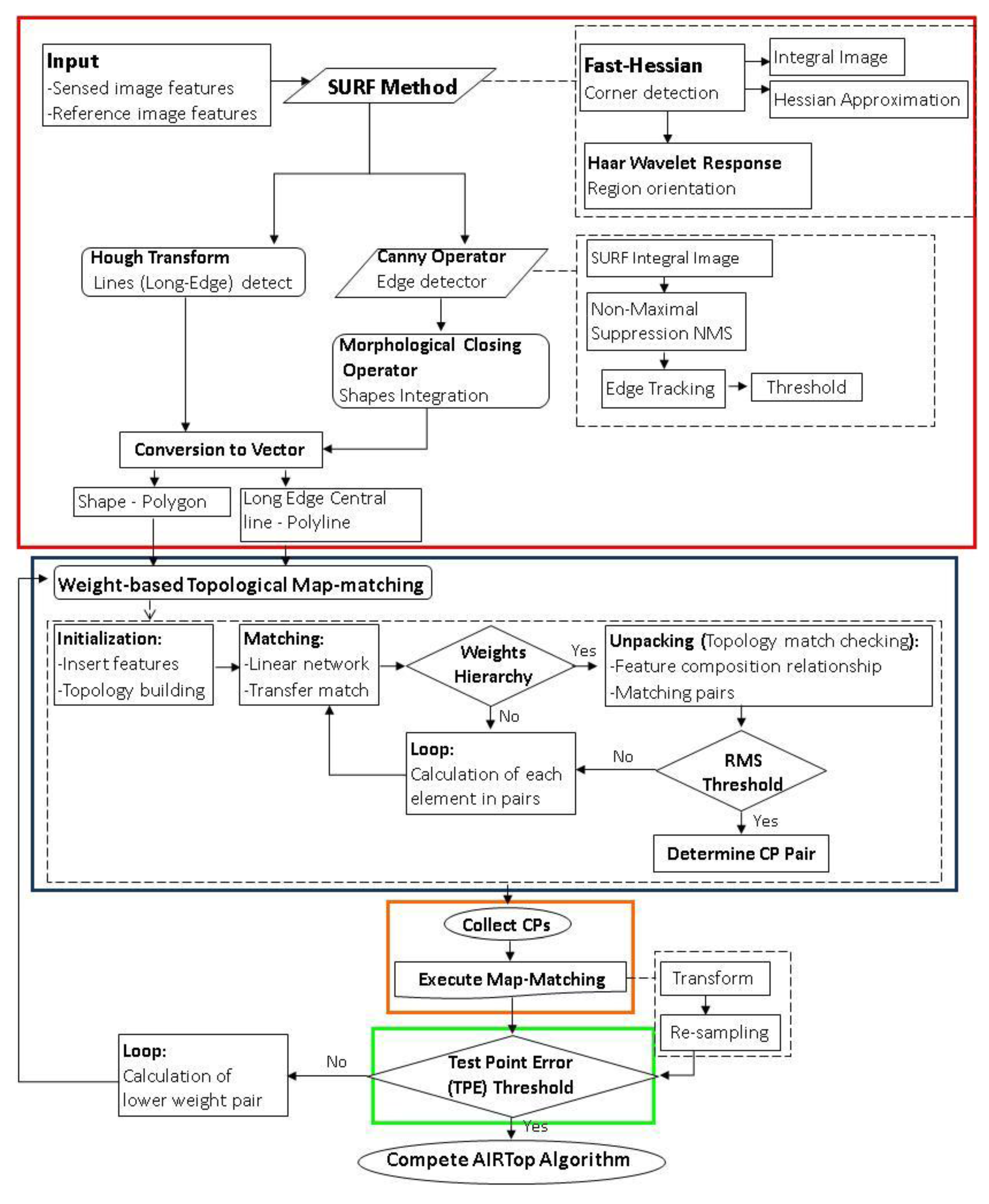
16], which is based on integral image and approximation, is performed. The Hessian matrix is responsible for primary image rotation (Figure 3) using principal points that are identified as being of interest. The next stage is to make a descriptor of local gray level geometry features. The vector representing the local feature is created by a combination of the Haar wavelet response. The values of dominant directions are defined relative to the principal point.
The approximated determinant of the Hessian represents the blob response in the image. These responses are saved in a blob response map over different scales, and local maxima are detected. An integral image (Equation (1)) at a location I   ( x ) represents the sum of all pixels in the input image I within a rectangular region formed by the origin and x . The sum of intensities inside a rectangular region (e.g., roofs) is calculated using integral images [17]:
Remotesensing 03 00065 i001
The Haar wavelet of the integral image is calculated. The responses are represented as points in a space with the horizontal response strength along the abscissa and the vertical response strength along the ordinate. The dominant orientation is estimated by calculating the sum of all responses within a sliding orientation window. The horizontal and vertical responses within the window are summed, yielding a local orientation vector. The longest vector defines the orientation of the point of interest [18].
The results of the SURF algorithm are three additional images (integral image, primary rotated image, and feature orientation image) of the reference and sensed images. The next stage is feature extraction from both the reference and sensed images, by applying two algorithms supported by the SURF algorithm images: The Hough Transform [19] used for long (global) edge extraction and the Canny detector [20] used for extraction of shorter (local) edges.
Figure 2. ROI selection. (A) Original image. (B) Entropy map of 10 adjacent blocks.
Remotesensing 03 00065 g002
Figure 3. Repeatability score for image rotation of up to 180°.
Remotesensing 03 00065 g003
The suggested process extracts long edges related to road features with the Hough Transform prior to the Canny operator. Since SURF integral (magnitude) and orientation images are applied as the base layer for feature detection, we propose modifying several stages of the Canny operator. First, the process of non-maximal suppression (NMS), also known as non-maximum, is imposed on the integral SURF image. Second, the edge-tracking process is controlled by a predefined threshold. The traditional Canny operator carries out the edge tracking according to a high and low (two) thresholds. The tracking of one edge begins at a pixel whose gradient is larger than the high threshold, and tracking continues in both directions from that pixel until there are no more pixels with gradients larger than the low threshold. However, it is usually difficult to set the two thresholds properly, especially for remotely sensed images, in view of the frequent nonuniformity of illumination and contrast in the different pixels [21]. In our method, the short (local) edges can be implemented without two predefined thresholds, as shown after using Hough Transform, relatively long edges are related to roof features.
Since it is difficult to detect continuous and stable edges solely from the images (reference and sensed), the morphological closing operation, produced by the combination of dilation and erosion operations, is employed. During this process, the edge detected areas are integrated into individual features. Finally, all of the extracted features are converted from raster to vector format and saved as a GIS project. While roofs are converted into polygons, roads are converted into polylines that cross along the central line of the detected (long edged) features.
The extracted features are enhanced using a thresholding program that creates a binary raster image. Vectors are then extracted from this binary image by use of a simplified chord test [22]. A pixel is considered to be part of the vector if the distance from its center to the vector being created is less than one pixel width. Modifications of the features include smoothing the vectors to remove or reduce the amount of aliasing so that they will have a more “real” appearance, or reducing the number of vertices (within vectors) produced during the initial translation.
A measure of the displacement between vector and initial raster feature provides more accurate information about the translations (Table 1). As the area of this study is large, representing mixed land uses and complex structures and shapes, we examined the accuracy of the vectorization/rasterization models (ArcMap 9.3, ESRI) based on simulated geometric data. This test quantified the amount of area committed/omitted/correctly assigned to the converted feature (from raster to vector and vice versa). This analysis was represented as an area error matrix.
Table 1. The error matrix for simulated geometric features (raster resolution 0.25 m; size 60 m × 60 m; square area is 9 m2; shape area is 7 m2; circle radius is 0.75 m with area of 1.77 m2) and commission/omission of errors (in m2).
Vector Data
Raster Data BackgroundSquareShapeCircle
Background 42.492840.0050.0020.0001642.5
Square0.0028.9980.0000.0009
Shape0.0040.0006.9960.0007
Circle0.001160.0000.0001.76841.77
42.59.0037.0161.76856

2.2. Topology Matching

Topological matching is used to reduce the search range or check the results of geometric matching since it is seldom used alone. Topological methods can spread the matching into the whole network, but this requires high topological similarity of the two datasets, as in topological transfer method [23].
The data pre-processing stage standardizes input data sets, and ensures that conflation data sets have the same data format and the same north direction (SURF-rotated image). As part of the preparation, the search key on the shapes must be defined. In a real data set, the features extracted from reference and sensed images are biased by noises and retained artifacts. Thus, out of the many possible methods for defining a search key, the selected method must include a succinct representation of the shape, and must not be sensitive to noise or small errors on the feature surface. We propose to use the Multiresolution Reeb Graph (MRG) skeleton structure method [24]. The Reeb graph uses a continuous scalar function on an object by the equivalence relation that identifies the points belonging to the same connected component [25].
In the topology-matching process, the Reeb graph is used as a search key that represents feature shapes. A node of the Reeb graph represents a connected component in a particular region, and adjacent nodes are linked by an edge if the corresponding connected components of the object are contiguous. The Reeb graph is constructed by repartitioning each region in a binary manner.
The output of the resampling process is a hierarchical design of nodes (base and support) for each extracted feature. Then, the integral of the geodetic distance is calculated using Dijkstra’s algorithm, which evaluates approximated values, as suggested by Hilaga et al. [26].
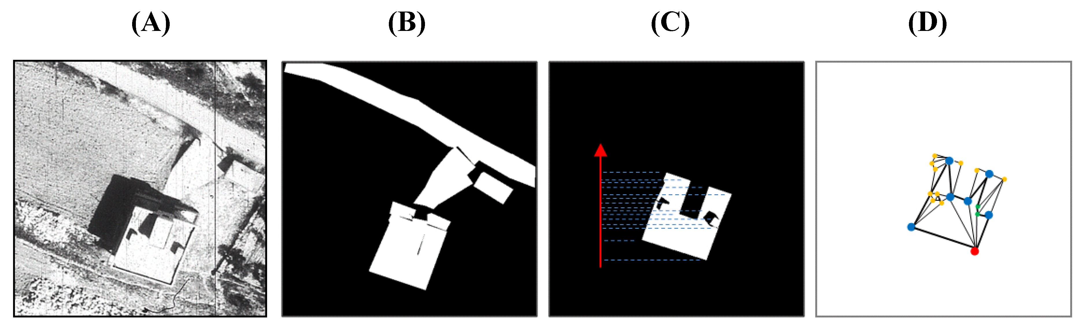
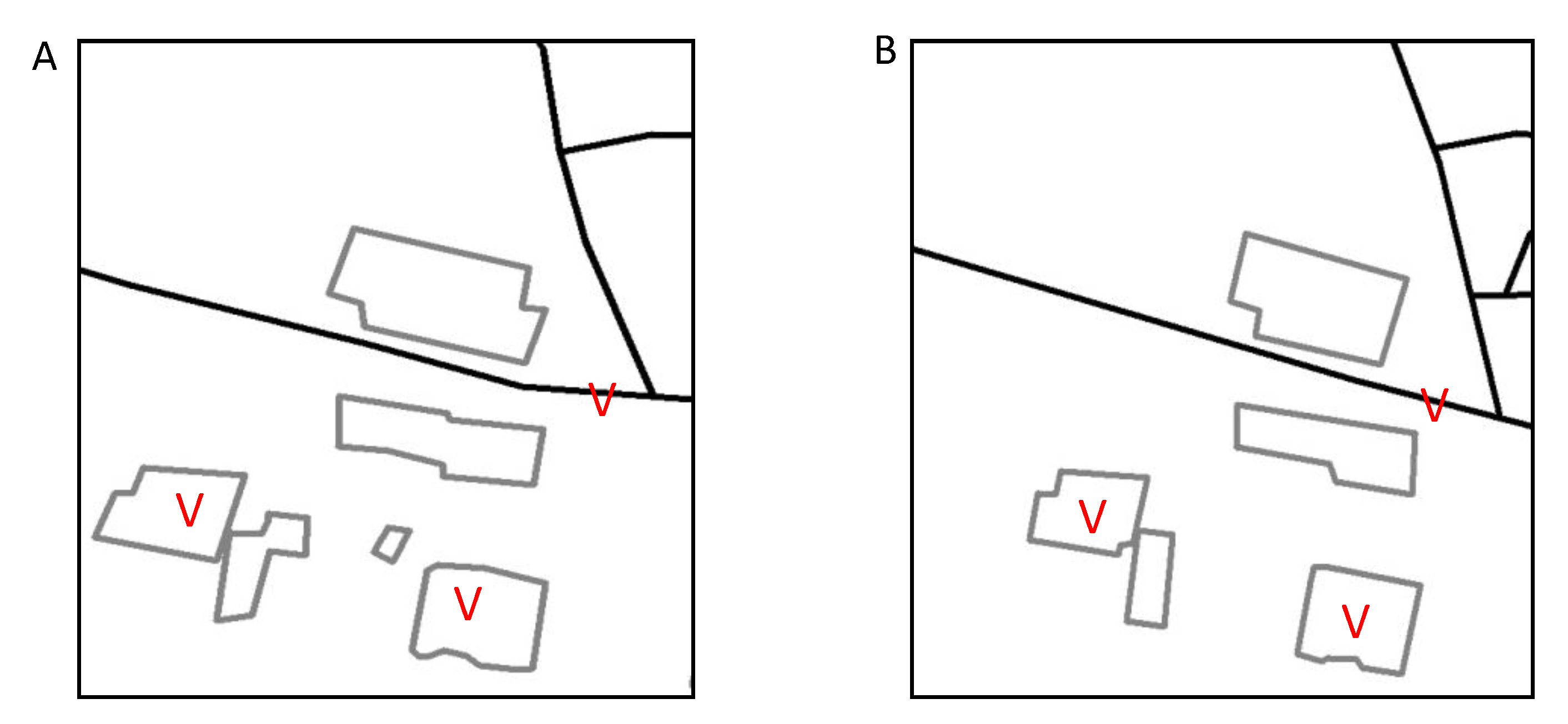
The construction of the MRG is illustrated in Figure 4. The following notations were defined: (1) R-node (red points are MRG node for s0 level, blue points for s1 level, green points for s3 level, orange points for s4 level); (2) R-edge (the thick lines connecting R-nodes of different resolutions); (3) T-set (the thin lines corresponding to each R-node in triangle connection); (4) μn-range (connecting function of R-node or T-set).
Figure 4. Multiresolution Reeb graph in 2D for a roof as the selected feature. (A) Original image; (B) map of extracted features; (C) selected feature with respect to the corner detection function; and (D) corresponding Reeb graph.
Remotesensing 03 00065 g004
Topology matching follows coarse-to-fine resolution levels to estimate similarities between features. The comparison between reference and sensed images is based on the vertex attributes (R-node, R-edge, T-set, and μn-range) of each feature in these images. The most influential R-node is selected based on hierarchy design for each feature separately. The record of these nodes is compared by attributes and summarizes to the matching list of candidate R-nodes. The matching process is guided by two rules for similarity: (1) How the final similarity is reduced by the matching; (2) adjacent effect of nearest R-nodes.

2.3. Weight-Based Topological Map-Matching

The MRG based approach has major limitations when used with airborne and spaceborne image registration and processing. This method is affected by connectivity within the feature surface and is not bound to represent the true skeleton of the features. Furthermore, it is sensitive to the geometry of the feature, and thus is not faithful to subgraph matching.
To overcome these limitations, we suggested formulating topology relations (connectivity and contiguity) between extracted features within reference and sensed images individually. According to the topology relation of polygon to polygon, polygon to polyline, and polyline to polyline, matching can be deduced. The topology rules that control the interaction between features are performed at two levels. In the first level, each feature is globally aware and related to all features within the image. In the second level, each feature is introduced to the nearest neighborhood and has knowledge of its local surroundings. This level overlaps with the ROI that was selected by adjacent small blocks during the feature-extraction stage.
Consider first how to formulate the spatial dependency and relation of a single image having n features. Since any error in the initial matching process will lead to mismatching of the CP positions, a robust three-stage approach is introduced. The first stage is identification of a set of candidate CPs. The following stages involve both reference and sensed images. The second stage is identification of correct CPs among candidate CPs using heading weight (Hw) and proximity weight (Pw). The final stage is to estimate similarity between selected features supported by the MRG skeleton structure.
First, the AIRTop algorithm creates an error tolerance around features, the radius of which is primarily based on spatial resolution of given image. All candidate CPs that are either within, crossing or tangent to the tolerance of a certain point are related to it and considered a suitable candidate. Identification of candidate CPs is established on the R-node for the s0 level (MRG nodes) of each feature. A set of candidate CPs is represented by the nodes and vertices of polygons (features related to roofs) and polylines (features related to roads).
Next, a square proximity matrix of the distances between features is created. We employ the Gaussian-weighted matrix using Chord Length Distribution (CLD) as suggested by Taylor and Cooper [27]. The heading is considered a cosine angle between features that has been included in a set of candidate CPs, in reference and sensed orientation (SURF result) maps. This parameter measures the angle difference between orientation maps with respect to the primary image rotation (SURF).
Finally, the similarity of the features is evaluated by MRG skeleton structure. The comparison includes all of the MRG parameters (R-node, R-edge, T-set and μn-range) for the features in both reference and sensed images.
The values of three weight coefficients (heading weight, proximity weight and MRG similarity) are estimated and summed to give the total weight score. The weight-optimization process parallels the map-matching (MM). The first feature is selected from a set of candidate CPs on the sensed image and compared to features on a set of reference images by the three spatial descriptions/attributes of the features. The process initiates with the first-level topology rules (in which features are related to an entire image), where feature attributes are global connectivity and contiguity matrices. The comparison at this level provides a temporal list of fitting CPs candidates from reference image for each feature in the sensed image. The process continues at the local level using the second level of topology rules (in which features are related to the nearest neighborhood), where feature attributes are local connectivity and contiguity matrices, proximity matrix, heading matrix and MRG parameters (for each feature individually). For a specific feature (in the sensed image), the optimization process starts with the map-matching of a positioning-fixed CP between sensed and reference images. If no fixed CPs are found, the algorithm continues to the next region of interest and candidate CPs are listed in the temporal file. In the case of fixed CPs, the random values for the three coefficients (heading weight (Hw), proximity weight (Pw) and MRG similarity) are generated between 1 and 100 (so that the sum of all coefficients equals 100). Using these values, the process then calculates the total weight score (MMtotal) for all features at the local level and indentifies the correct CPs based on the highest total weight score value (Equation (2)):
Remotesensing 03 00065 i002
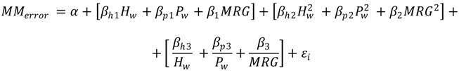
The relationship between percentage of wrong CPs identified and the weight coefficients (heading weight (Hw), proximity weight (Pw) and MRG similarity) is developed using a regression analysis. Since the functional relationship between the weights and the map-matching error is an internal test for accuracy, various specifications are considered. We assumed that the map-matching depends on the individual weights (Hw, Pw, MRG), their square terms and their inverse terms. In Equation (3), α is a selected point, β are the regression coefficients to be estimated and ε i is the error of rasterization/vectorization conversion that has been assumed to be independently and identically distributed with constant variance:
Remotesensing 03 00065 i003
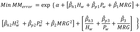
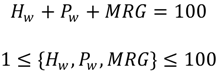
To minimize the error, some restrictions have to be imposed. As discussed, the sum of all weight coefficients is set to 100 and the minimum and maximum values of each weight coefficient are set at 1 and 100, respectively. The optimization function obtained from the MMerror analysis is given in Equation (4):
Remotesensing 03 00065 i004
subject to:
Remotesensing 03 00065 i005
Equation (4) was optimized using the nonlinear minimization method proposed by Michael et al. [28]. The values of the weight coefficients were calculated by identifying the global minimum of the map‑matching stage.
The accuracy of the map-matching procedure is estimated by mathematical representation of RMSE value. The results of the local map-matching are determined by a predefined RMSE threshold that is dependent on the spatial resolution of the images in question. If the algorithm fails to identify the correct CPs among the candidate features and the RMSE exceeds the threshold, then the algorithm regenerates another set of random values of coefficients and repeats the map-matching. This process continues by optional loop procedure until the algorithm selects the correct CPs.
To determine the accuracy of the map-matching procedure, we modified the commonly used test Point Error (TPE) method [15]. TPE defines the test set by excluding groups of CPs from the map‑matching procedure and measures the accuracy of the registration process. Our modification of the TPE uses marked features rather than fixed CPs. These features are randomly chosen from the extracted-features map according to ROI. As a result, no regions are marked due random selection mode. Our scoring method does not allow setting TPE to zero due to overfitting. In our algorithm, 10% of all CPs are excluded as a test set from TPE evaluation. Again, if the algorithm fails to transform and resample the sensed image and TPE exceeds the threshold, then the algorithm regenerates by optional loop procedure.
For a given level of detail, the inner loop of the algorithm, as indicated in Figure 1, optimizes the registration process in the global and local image domains. By globally optimizing the corresponding ROIs, the optimization process can rapidly converge or even skip areas that do not contain a required feature, leading to considerable savings in execution time. The strategy of local registration by global optimization can be justified by the following facts. If the CPs are already close to their optimal position within the selected ROI, the separated optimization of each CP leads to the same solution as the optimization of all points within the selected ROI. The optimal value of the similarity is achieved by maximizing the local topological relation of each component to the global similarity of the ROIs. The contributions of topological relation to each ROI are independent of each other because they are achieved by small rearrangements of the CPs, which adjust the registration of both images in local areas.

3. Results

This section presents both simulated and real-world results. First, we evaluate the effect of multi-temporal parameter settings and show the overall performance of the suggested AIRTop algorithm using a standard evaluation set. Then, we evaluate the effect of multi-temporal and multi-sensor parameters. AIRTop has already been tested in a few real-world applications. Taking this application further, we focus in this article on the more difficult problem of camera calibration and temporal changes. AIRTop manages to calibrate the camera reliably and accurately, even in some very challenging cases.

3.1. Experimental Evaluation

One important advantage of simulated images is that they help meet the basic requirement for the automatic image registration algorithm that nothing is misleading between local and global registration accuracies. One drawback of the global topology method is that when the image has local geometric differences or the CPs in a local neighborhood are inaccurate, the local geometric differences average out equally over the whole image. The effect of geometric differences or measurement inaccuracy of a CP on an approximating point will be the same no matter how near or far the CP is from the approximating point. Thus, the AIRTop algorithm uses an improved method in which a CP influences the nearby point more than distant points. To localize this method, we define a weight function that represents the contribution or influences of the CPs by weight-based topology.
Note that for every point, we have an error measure in the form of RMSE; by minimizing the error measure, we obtain a mapping function that best fits the data when considered from the selected point. Thus, for each candidate point in the reference image, we are determining the corresponding component point in the sensed image. The overall accuracy of the map-matching procedure is provided by the TPE.
This section describes a set of simulated images which make it possible to evaluate the matching accuracy of the proposed technique. The strategy of testing the AIRTop algorithm using simulated images emphasizes the following: (1) Temporal changes simulated by adding and removing structures and lines; (2) multi-sensor data simulated by different spatial resolutions (rotation and scaling). The evaluation criterion is the repeatability score. We estimated the temporal changes between two images by adding and removing features from the attribute table (in ARCGIS) using a statistical random code. From the captured images, we extracted 15 to 21 ROIs having 108 to 58 features, which were used for the registration experiments. These ROIs contain only polygons and polylines, and they do not contain any background. We launched the AIRTop algorithm between a reference image before the random function and after it. We estimated the TPE (Test Point error for 10% of all CP pairs) by matching images on the weighting function used in each ROI, where each CP pair was optimized by RMSE threshold for every experimental image.
We evaluated the errors in the following manner: 43 images of random changes were matched to a reference image. Figure 5 shows that the TPE, with a reasonable accuracy rate of >0.9, is maintained for a temporal change rate of <40% in 26 simulated scenarios of spatial variances, including feature deletion and displacement. For cardinal changes (>40%), the RMSE threshold in stage 2 (topological map matching) fails to identify the correct CP pair.
Figure 5. Temporal change versus registration accuracy. Blue points are different simulations of temporal changes, the black hatched line is the trend line, and the red arrow is the RMSE threshold of the topological map-matching stage.
Remotesensing 03 00065 g005
Artificial scaling and rotation of a simulated image is used to evaluate the matching accuracy for a multi-sensor data set. Table 2 summarizes the displacement error, where TPE represents Test Point error for 10% of all CP pairs. “Original” corresponds to the original spatial resolution (0.1 m) and orientation (0°) of the simulated image and reference image matched to itself (after rasterization/vectorization procedure); “Sim1” corresponds to a rotation of 100°, “Sim1_1” corresponds to a rotation of 100° and 2X scaling , “Sim2” corresponds to a rotation of 290°, “Sim2_2” corresponds to rotation of 290° and 2.5X scaling.
Table 2. Error (in m) for a simulated multi-sensor data set with an original image resolution of 0.1 m and orientation of 0°.
Simulated data setOriginalSim 1Sim 1_1Sim 2Sim 2_2
TPE0.010.0320.0560.0380.063
The parameters shown in Table 2 were selected by experimental optimization using the topology weighting function. By changing the parameters of the weighting function, we could reduce the estimated error and achieve relatively high accuracy.

3.2. Case Study Using Real Images

In this study, we selected three sensors to emphasize the multi-sensor registration at two selected periods in which multi-temporal changes occurred. The selected sensors are documented in Table 3. Images of these three sensors covered an area of 1.5 × 1.1 km in central (33°30′/34°42′) Israel.
Table 3. Selected sensors.
SensorTypeDetectorSpatial ResolutionRadiometric ResolutionDate
IkonosSpacebornePushbroom1 m11 bit06/2008
Panchromatic scanner 1AirbornePushbroom0.25 m12 bit07/2009
Panchromatic scanner 2AirborneWhiskbroom0.12 m8 bit06/2009
Panchromatic scanner 2AirborneWhiskbroom0.12 m8 bit02/2009
Prior to feature detection, the ROIs, which contain relatively large radiometric variation (grayscale contrasts), were selected. For viewing convenience, the results of the AIRTop algorithm are presented for a selected ROI (Figure 6). The next stage, illustrated in Figure 7, was feature extraction for a panchromatic airborne scanner from both the reference image (from 06/2009 with 0.12 m spatial resolution) and the sensed image (from 07/2009 with 0.25 m spatial resolution), applying two algorithms (Hough Transform and Canny) supported by SURF images (integral and orientation).
Figure 6. The selected ROI. (A) Original reference image; (B) Entropy image.
Remotesensing 03 00065 g006
Figure 7. Buildings (gray polygons) and roads (black polyline) extraction for: (A) The reference image (panchromatic airborne scanner with spatial resolution of 0.12 m from 06/2009); and (B) the sensed image (panchromatic airborne scanner with spatial resolution of 0.25 m from 07/2009).
Remotesensing 03 00065 g007
The next stages were performed automatically: our algorithm searches for corresponding CP pairs, applying weighting function and topology. In the presented case study, the AIRTop successfully detected three matched features (marked V in Figure 7) and exposed seven CPs. The final results of the image registration procedure are shown in Figure 8. The TPE for 18 CPs, which are 10% of all the detected CPs, was 0.043 m.
The suggested procedure was used for registration between an Ikonos (spaceborne) image and three panchromatic (airborne) images (Table 3). The errors in displacement of the three sensed panchromatic images to the reference Ikonos image from 2008 are summarized in Table 4. Values represent TPE for 10% of all CP pairs.
Figure 8. Results of the image-registration process with the AIRTop algorithm between: (A) Reference image (panchromatic airborne scanner with spatial resolution of 0.12 m from 06/2009); and (B) sensed image (panchromatic airborne scanner with spatial resolution of 0.25 m from 07/2009). (C) Image produced by the registration procedure showing overlap between reference and sensed images (with transparency of 30%).
Remotesensing 03 00065 g008
Table 4. Error (in m) for the three panchromatic (airborne) images (with spatial resolution of 0.12 m and 0.25 m) matched to Ikonos (spaceborne) image (with spatial resolution of 1 m) with 180 CPs.
Sensed imagePanchromatic scanner 1 (07/2009)Panchromatic scanner 2 (06/2009)Panchromatic scanner 2 (02/2009)
TPE1.130.740.4

4. Discussion

In this paper, a new technique for an automated image registration algorithm is presented. Our study focused on the registration of multi-sensor and multi-temporal images. We proposed combining the image-processing and map-matching procedures, and incorporating tools of remote sensing and GIS, into an automatic method for image registration. The suggested algorithm proved able to register two images acquired from different sensors (airborne and spaceborne), and from different periods, and hence different viewpoints, which are expected to be dissimilar in rotation, translation, and possible scaling.
According to the literature, many existing algorithms suffer from two main problems: Errors caused by different intensities between images and therefore inability to handle multi-sensor and multi-temporal (multimodal) data sets; and computation power limits.
To overcome these, we proposed to extract features for the reference and sensed images, convert them to GIS vector maps, and use these for the registration procedure. Operating on feature maps instead of the image itself not only solves the correlation limitation (correlating intensity values), but also reduces computational requirements since most of the map, aside from the feature locations, consists of zero values.
The notion of addressing the registration problem by applying a global-to-local level strategy provided an elegant method to speed up the whole process, while enhancing the accuracy of the registration procedure. What we found is that when using the global level for map-matching, the AIRTop fails to consistently give good registration results. This was improved by reducing the area to ROIs, which were selected based on an entropy map. The significant reduction in data points greatly reduced the computation time required for the algorithm.

References and Notes

  1. Moigne, J.L.; Campbel, W.J.; Cromp, R.F. An automated parallel image registration technique based on the correlation of wavelet features. IEEE Trans. Geosci. Remote Sens. 2002, 40, 1849–1864. [Google Scholar] [CrossRef]
  2. Brown, L.G. A survey of image registration techniques. ACM Comput. Surv. 1992, 24, 325–376. [Google Scholar] [CrossRef]
  3. Zitova, B.; Flusser, J. Image registration methods: A survey. Imag. Vis. Comput. 2003, 21, 977–1000. [Google Scholar] [CrossRef]
  4. Fonseca, L.; Costa, M. Automatic Registration of Satellite Images. In Proceedings of Brazilian Symposium on Computer Graphics and Image Processing, Campos do Jordao, Brazil, October 14–17, 1997; pp. 219–226.
  5. Viola, P.; Wells, W.M. Alignment by maximization of mutual information. Int. J. Comput. Vis. 1997, 24, 137–154. [Google Scholar] [CrossRef]
  6. Wu, J.; Chung, A. Multimodal Brain Image Registration Based on Wavelet Transform Using SAD and MI. In Proceedings of the Second International Workshop on Medical Imaging and Augmented Reality, Beijing, China, August 19–20, 2004.Medical Imaging and Augmented Reality: Second International Workshop, MIAR 2004, Beijing, China, August 19-20, 2004, Proceedings; Yang, G.; Jiang, T. (Eds.) LNCS; Springer: Berlin/Heiderberg, Germany, 2004; Volume 3150, pp. 270–277.
  7. Fan, X.; Rhody, H.; Saber, E. Automatic Registration of Multi-Sensor Airborne Imagery. In Proceedings of 34th Applied Imagery and Pattern Recognition Workshop, Washington, DC, USA, December 1, 2005; pp. 80–86.
  8. Zavorin, I.; Le Moigne, J. Use of multiresolution wavelet feature pyramids for automatic registration of multisensor imagery. IEEE Trans. Image Process. 2005, 14, 770–782. [Google Scholar] [CrossRef] [PubMed]
  9. Xu, R.; Chen, Y. Wavelet-based multiresolution medical image registration strategy combining mutual information with spatial information. Int. J. Innov. Comput. Inf. Control 2007, 3, 285–296. [Google Scholar]
  10. Anderson, T.W. An Introduction to Multivariate Statistical Analysis; Wiley: New York, NY, USA, 1950; pp. 75–78. [Google Scholar]
  11. Chantous, M.; Ghosh, S.; Bayoumi, M. A Multi-Modal Automatic Image Registration Technique based on Complex Wavelets. In Proceedings of 16th IEEE International Conference on Image Processing, Cairo, Egypt, November 7–10, 2009; pp. 173–176.
  12. Jensen, J.R. Introductory Digital Image Processing, 3rd ed.; Prentice Hall: Upper Saddle River, NJ, USA, 2004. [Google Scholar]
  13. Bay, H.; Ess, A.; Tuytelaars, T.; Van Gool, L. Speeded-Up Robust Features (SURF). Comput. Vis. Image Understand. 2008, 110, 346–359. [Google Scholar] [CrossRef]
  14. Velaga, N.R.; Quddus, M.A.; Bristow, A.L. Developing an enhanced weight-based topological map-matching algorithm for intelligent transport systems. Transp. Res. C-Emerg. Technol. 2009, 17, 672–683. [Google Scholar] [CrossRef] [Green Version]
  15. Greenfeld, J.S. Matching GPS Observation to Location on a Digital Map. In Proceedings of 81st Annual Meeting of the Transportation Research Board, Washington, DC, USA, January 13–17, 2002.
  16. Florack, L.M.J.; ter Haar Romeny, B.M.; Koenderink, J.J.; Viergever, M.A. General intensity transformations and deferential invariants. J. Math. Imag. Vis. 1994, 4, 171–187. [Google Scholar] [CrossRef]
  17. Brown, H.; Lowe, D. Invariant Features from Interest Point Groups. In Proceedings of British Machine Vision Conference 2002, Cardiff, Wales, UK, September 2–5, 2002; pp. 656–665.
  18. Lindeberg, T. Feature detection with automatic scale selection. Int. J. Comput. Vis. 2004, 30, 79–116. [Google Scholar] [CrossRef]
  19. Duda, R.O.; Hart, P.E. Use of the Hough transform to detect lines and curves in pictures. Commun. ACM 1972, 15, 11–15. [Google Scholar] [CrossRef]
  20. Canny, J. A computational approach to edge detection. IEEE Trans. Pattern Anal. Mach. Intell. 1986, 8, 679–698. [Google Scholar] [CrossRef] [PubMed]
  21. Simard, P.; Bottou, L.; Haffner, P.; LeCun, Y. Boxlets: A Fast Convolution Algorithm for Signal Processing and Neural Networks. In Proceedings of the 1998 Conference on Advances in Neural Information Processing Systems II, Denver, CO, USA, November 30–December 5, 1998; pp. 571–577.
  22. Congalton, R.G. Exploring and evaluating the consequences of Vector-to-Raster and Raster-to-Vector conversion. Photogram. Eng. Remote Sensing 1997, 63, 425–434. [Google Scholar]
  23. Tomaselli, L. Topological Transfer: Evolving Linear GIS Accuracy. In Proceedings of URISA 1994 Conference Proceeding, Milwaukee, WI, USA, November 1994; pp. 245–259.
  24. Iyer, N.; Jayanti, S.; Lou, K.; Kalyanaraman, Y.; Ramani, K. Three-dimentional searching: State-of-the-art and future trends. Comput. Aid. Des. 2005, 37, 509–530. [Google Scholar] [CrossRef]
  25. Blum, H. A transformation for extracting new descriptors of shape. In Models for the Perception of Speech and Visual Form; Wathen-Dunn, W., Ed.; MIT Press: Cambridge, MA, USA; 1967; pp. 362–380. [Google Scholar]
  26. Hilaga, M.; Shinagawa, Y.; Kohmura, T.; Kunii, T.L. Topology Matching for Fully Automatic Similarity Estimation of 3D Shapes. In SIGGRAPH ’01 Proceedings of the 28th Annual Conference on Computer Graphics and Interactive Techniques, Los Angeles, CA, USA, August 12–17, 2001; pp. 203–212.
  27. Taylor, C.J.; Cooper, D.H. Shape Verification Using Belief Updating. In Proceeding of 1st British Machine Vision Conference, Oxford, UK, September 24–27, 1990; pp. 61–66.
  28. Michael, C.F.; Mangasarian, O.L.; Wright, S.J. Linear Programming with MATLAB; MPS-SIAM Series on Optimization; Society for Industrial and Applied Mathematics: Philadelphia, PA, USA, 2007. [Google Scholar]

