What Do Observational Datasets Say about Modeled Tropospheric Temperature Trends since 1979?

Abstract
:1. Introduction
2. Data

| Name | Version | Instrumentation | Citation | Notes |
|---|---|---|---|---|
| HadAT | 2 | Radiosonde | [27] | Breakpoints and adjustments calculated from adjacent radiosondes and metadata (Hadley Centre Atmospheric Temperatures) |
| RATPAC | Radiosonde | [28,29] | Breakpoints and adjustments calculated from adjacent radiosondes, metadata and expert opinion (Radiosonde Atmospheric Temperature Products for Assessing Climate) | |
| RAOBCORE | 1.4 | Radiosonde | [30] | Breakpoints and adjustments calculated from first guess of ERA-40 Reanalyses. (RAdiosonde OBservation COrrection using REanalyses) |
| RICH | Radiosonde | [30] | Breakpoints calculated from ERA-40, adjustments calculated from adjacent radiosondes (Radiosonde Innovation Composite Homogenization) | |
| UAH | 5.3 | Microwave | [9] | Polar orbiting microwave sensors. (University of Alabama in Huntsville) |
| RSS | 3.2 | Microwave | [21] | Polar orbiting microwave sensors. (Remote Sensing Systems) |
| AS08 | Radiosonde wind | [15] | Thermal wind relationship (Allen and Sherwood 2008 [15]) | |
| C10 | Radiosonde wind | This paper (C10) | Thermal wind relationship | |
| ERA-I | ERA-INTERIM | Reanalysis | [20] | Model assimilation of multiple observational products 1989-2009 only (European Centre ReAnalysis project) |
| Tsfc | ||||
| ERSST | 3b | Thermometers | [31] | Includes land values (Extended Reconstruction Sea Surface Temperature —NOAA) |
| HadCRUT | 3v | Thermometers | [32] | Anomalies are adjusted for consistent variances through time (little impact on post-1979 data). (Hadley Centre and Climate Research Unit) |
| GISS | LOTI | Thermometers | [33] | 24°S–24°N (Goddard Institute for Space Studies—NASA) |
2.1. Radiosonde: HadAT, RATPAC, RAOBCORE, RICH
2.2. Satellite: UAH, RSS
2.3. Thermal Wind: AS08, C10
2.4. Surface: ERSST, HadCRUT, GISS
3. Results


3.1. Assessments of the Products
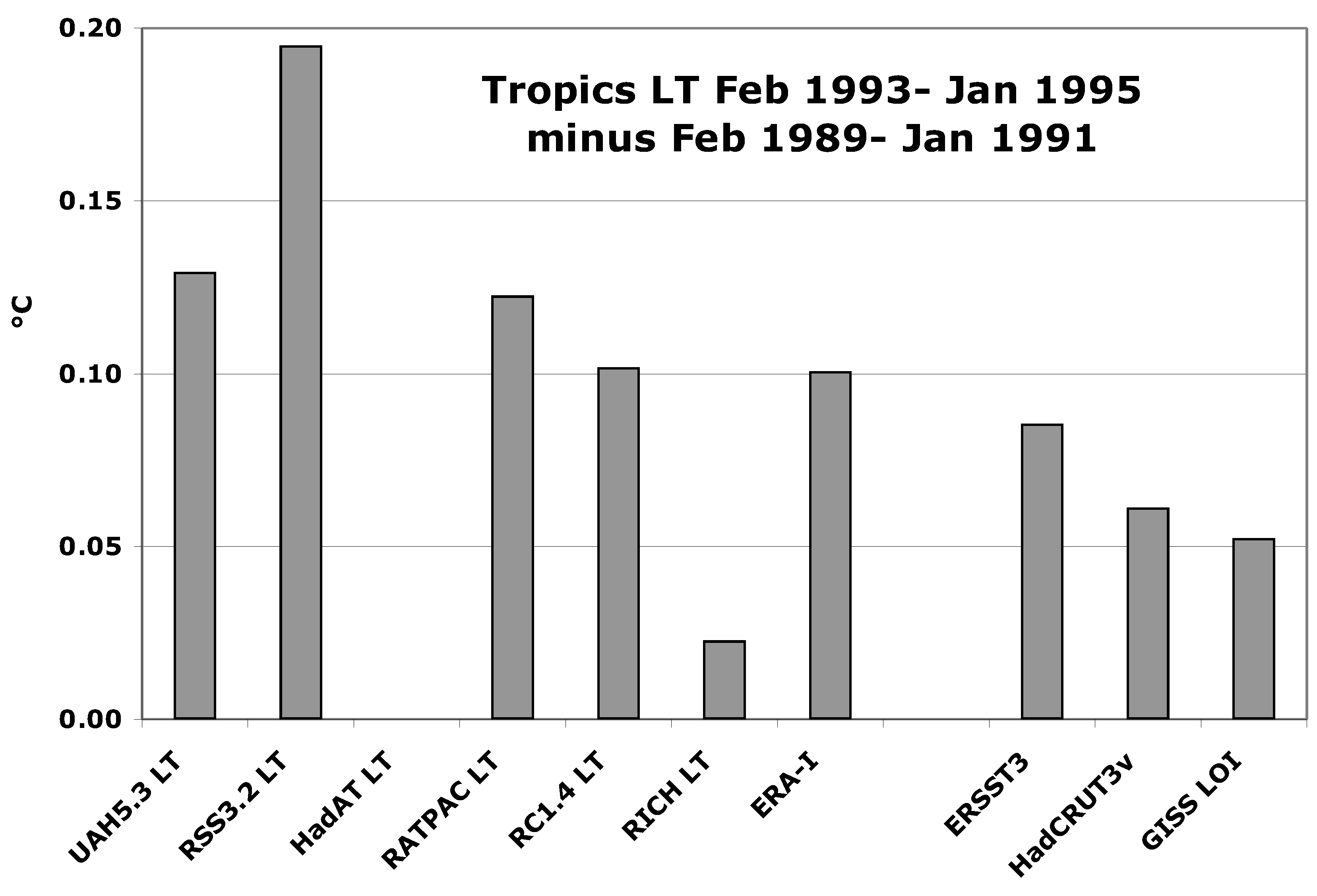
3.1.1. Radiosonde
3.1.2. Satellite
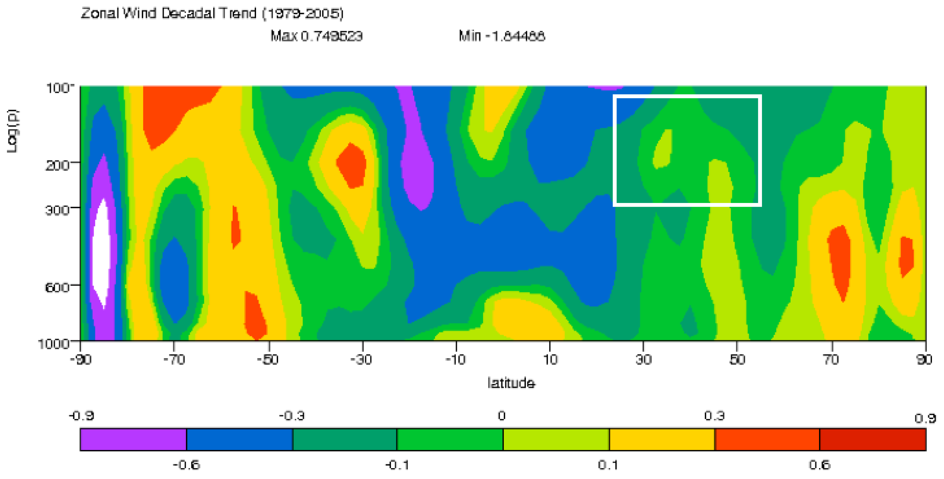
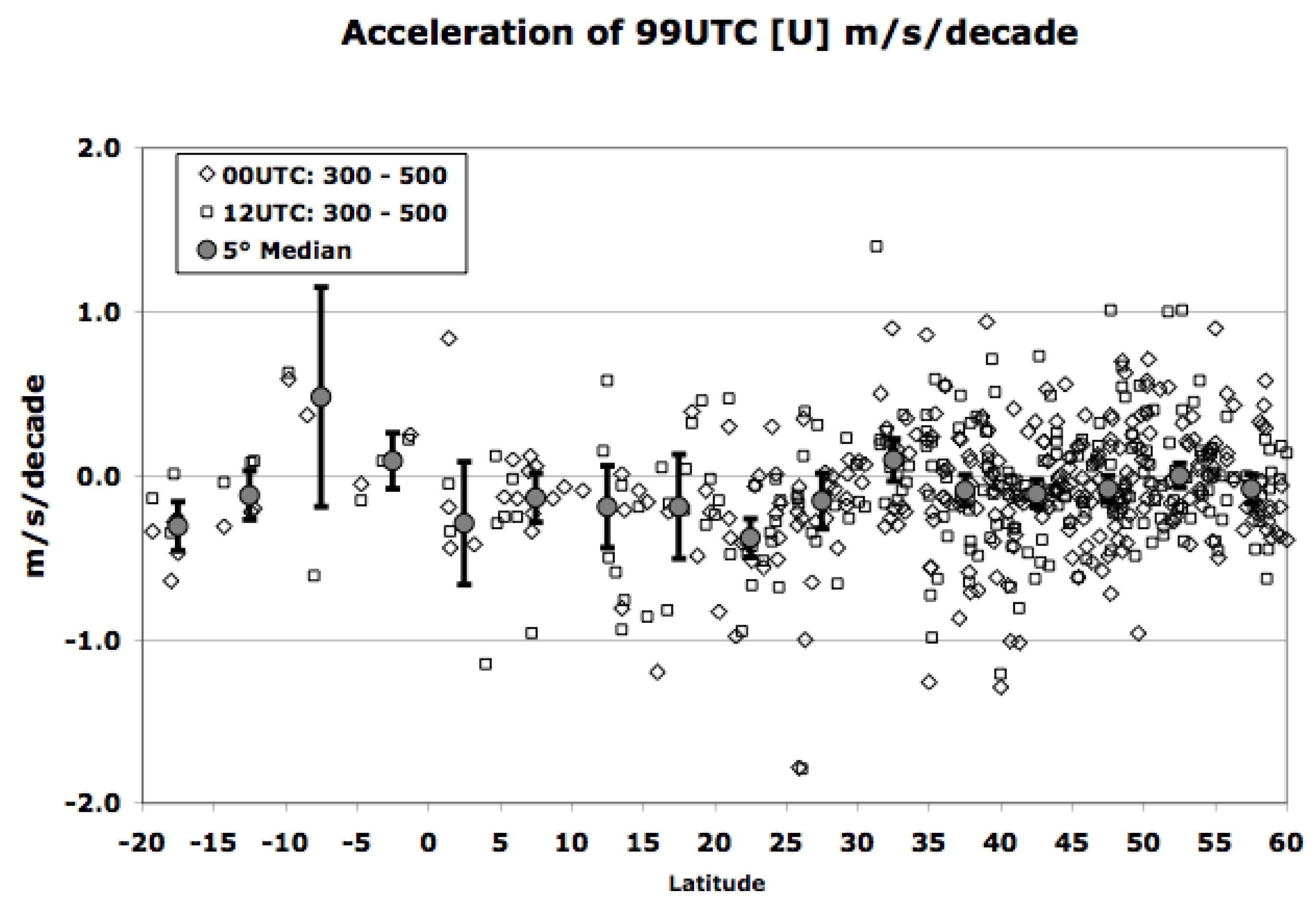
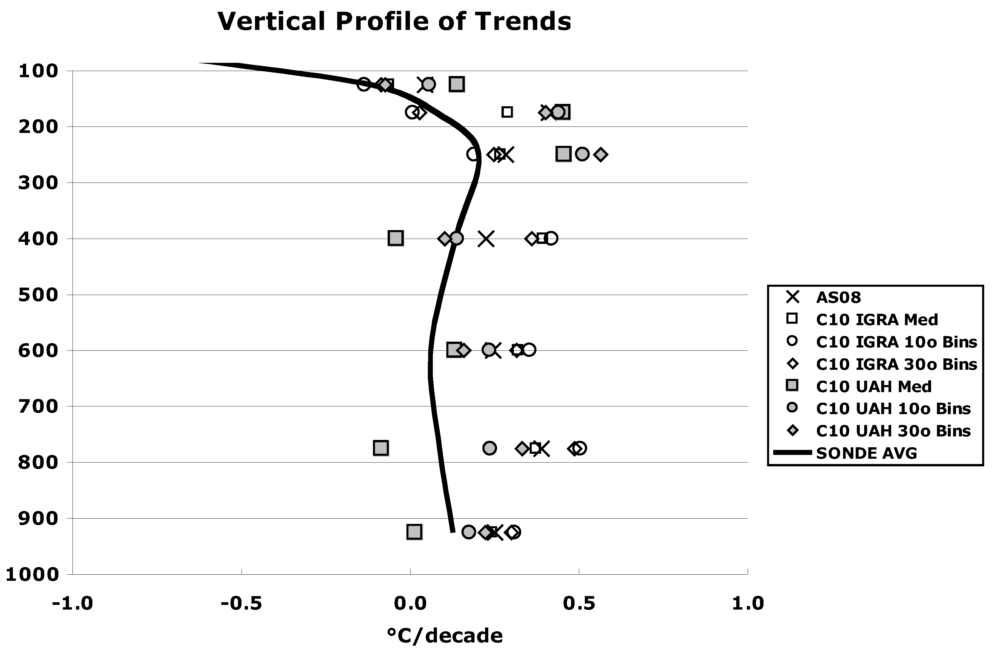
3.1.3. Thermal Wind
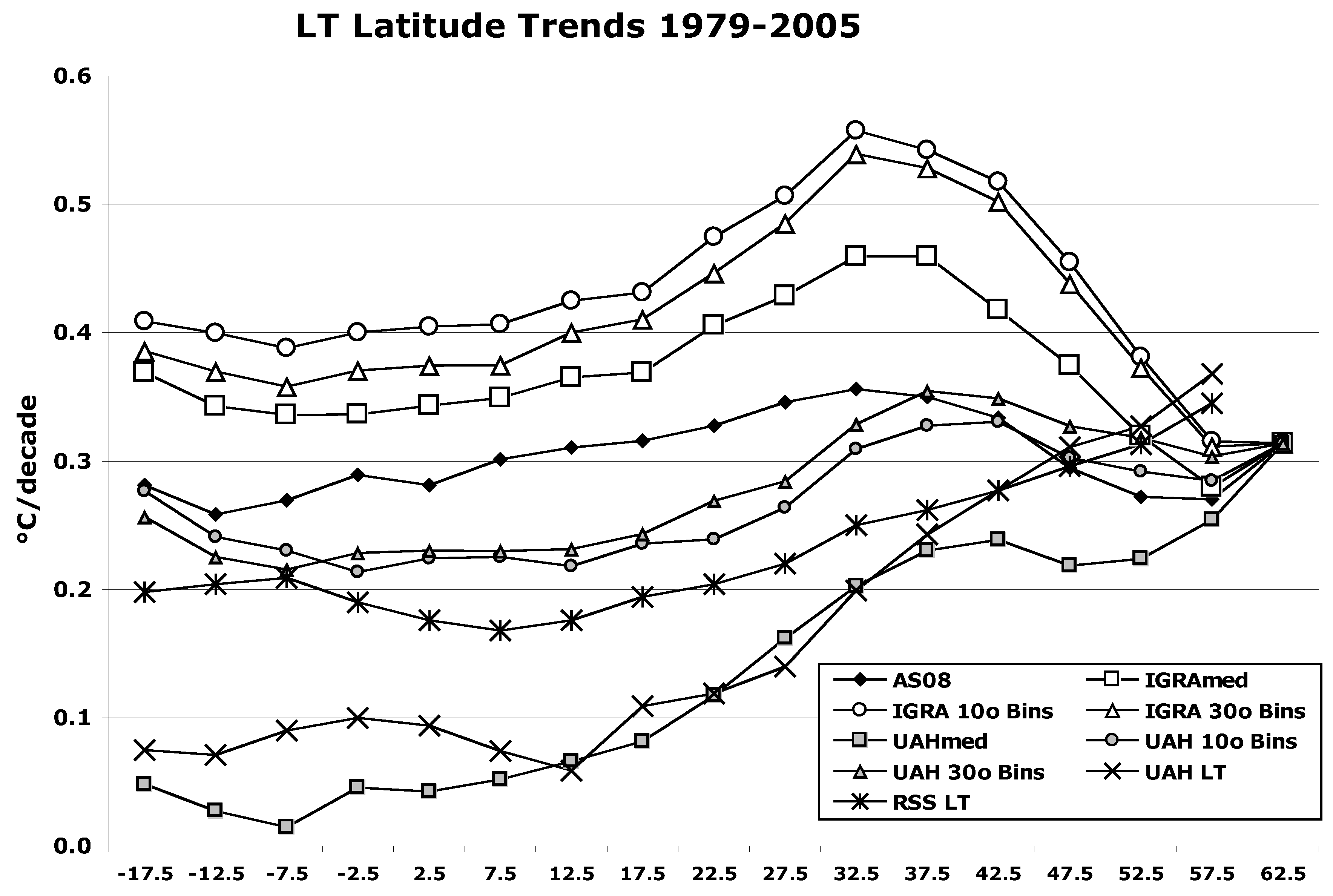
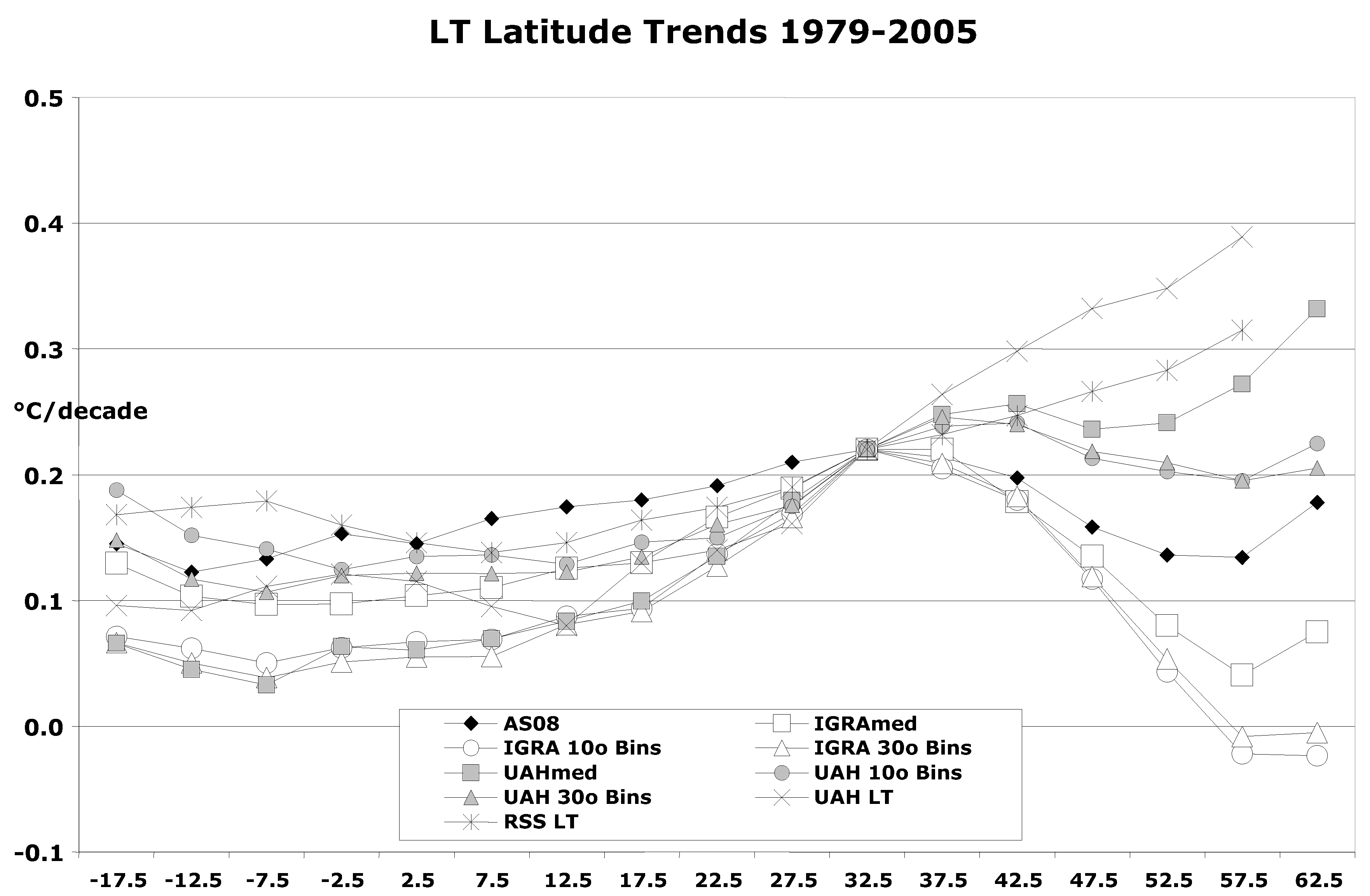
3.1.4. Determining “Best Guess”
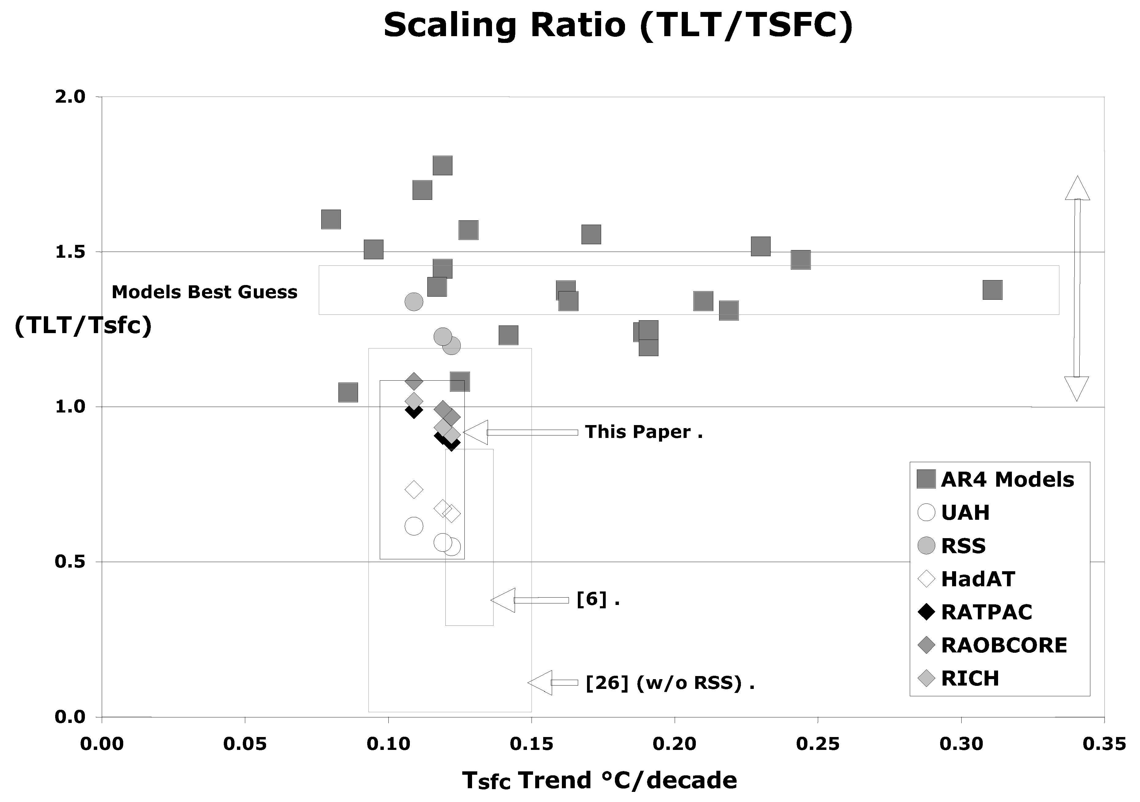
3.2. The Scaling Ratio
| Tsfc/TLT | ERSST [+0.122] | HadCRU [+0.119] | GISS [+0.109] |
|---|---|---|---|
| UAH [+0.067] | 0.55 | 0.56 | 0.61 |
| RSS [+0.146] | 1.20 | 1.23 | 1.34 |
| HadAT [+0.080] | 0.66 | 0.67 | 0.73 |
| RATPAC [+0.108] | 0.89 | 0.91 | 0.99 |
| RAOBCORE [+0.118] | 0.97 | 0.99 | 1.08 |
| RICH [+0.111] | 0.91 | 0.93 | 1.02 |
| Best Guess [+0.09 ±0.03] | 0.74 0.49 − 0.98 | 0.76 0.51 − 1.01 | 0.83 0.55 − 1.10 |
| AS08 [+0.288] | 2.10* | 2.11* | 2.23* |
| C10 [+0.275] | 2.01* | 2.02* | 2.13* |
| Best Estimate | Spread | ||
| AR4 Models | 1.38 1.30 − 1.46 | 1.38 1.00 − 1.76 |

[Note: if we collapse Figure 10 to the left axis to make a histogram of occurrences of model and observed SRs, we can apply a Chebyshev’s test of inequality assuming that the resulting distribution of observational results is not “normal.” This much less restrictive test indicates that there is a 12% chance that the observed SR (without RSS) is greater than 1.20 even though none of the 15 samples reached this value. However, the model distribution of values is indeed “normal” which implies a probability of only 2.5% that the model SR is less than 1.00. Thus a statement that the average model SR is significantly different from observed SRs holds, but that a small sample of individual model SRs do overlap with some of the observed SRs. On the other hand, none of the model SRs overlap with SRs from UAH, HadAT and RATPAC.]
4. Conclusions
References
- Christy, J.R.; McNider, R.T. Satellite greenhouse signal. Nature 1994, 367, 325. [Google Scholar] [CrossRef]
- Douglass, D.H.; Christy, J.R.; Pearson, B.D.; Singer, S.F. A comparison of tropical temperature trends with model predictions. Int. J. Climat. 2007. [Google Scholar] [CrossRef]
- Karl, T.R.; Hassol, S.J.; Miller, C.D.; Murray, W.L. Temperature Trends in the Lower Atmosphere: Steps for Understanding and Reconciling Differences; U.S. Climate Change Science Program Synthesis and Assessment Product 1.1; The Climate Change Science Program and the Subcommittee on Global Change Research: Washington, DC, USA, 2006. [Google Scholar]
- Santer, B.D.; Thorne, P.W.; Haimberger, L.; Taylor, K.E.; Wigley, T.M.L.; Lanzante, J.R.; Solomon, S.; Free, M.; Gleckler, P.J.; Jones, P.D.; Karl, T.R.; Klein, S.A.; Mears, C.; Nychka, D.; Schmidt, G.A.; Sherwood, S.C.; Wentz, F.J. Consistency of modelled and observed temperature trends in the tropical troposphere. Int. J. Climatol. 2008. [Google Scholar] [CrossRef]
- Thorne, P.W. Atmospheric science: The answer is blowing in the wind. Nature Geosci. 2008. [Google Scholar] [CrossRef]
- Christy, J.R.; Norris, W.B.; Spencer, R.W.; Hnilo, J.J. Tropospheric temperature change since 1979 from tropical radiosonde and satellite measurements. J. Geophys. Res. 2007, 112, D06102. [Google Scholar] [CrossRef]
- Klotzbach, P.J.; Pielke, R.A., Sr.; Christy, J.R.; McNider, R.T. An alternative explanation for differential temperature trends at the surface and in the lower troposphere. J. Geophys. Res. 2009. [Google Scholar] [CrossRef]
- Klotzbach, P.J.; Pielke, R.A., Jr.; Christy, J.R.; McNider, R.T. Correction to “An alternative explanation for differential temperature trends at the surface and in the lower troposphere.”. J. Geophys. Res. 2010. [Google Scholar] [CrossRef]
- Christy, J.R.; Spencer, R.W.; Norris, W.B. The role of remote sensing in monitoring global bulk tropospheric temperatures. Int. J. Rem. Sens. 2010. In press. [Google Scholar] [CrossRef]
- McKitrick, R.; McIntyre, S.; Herman, C. Panel and multivariate methods for tests of trend equivalence in climate data series. Atmos. Sci. Lett. 2010. In press. [Google Scholar] [CrossRef]
- Randel, W.J.; Wu, F. Biases in stratospheric and tropospheric temperature trends derived from historical radiosonde data. J. Climate 2006, 19, 2094–2104. [Google Scholar] [CrossRef]
- IPCC AR4. Climate Change 2007: The Physical Science Basis. Contribution of Working Group I to the Fourth Assessment Report of the Intergovernmental Panel on Climate Change; Soloman, S., Qin, D., Manning, M., Chen, Z., Marquis, M., Averyt, K.B., Tignor, M., Miller, H.L., Eds.; Cambridge University Press: Cambridge, UK and New York, NY, USA, 2007. [Google Scholar]
- Christy, J.R.; Norris, W.B. Discontinuity issues with radiosonde and satellite temperatures in the Australian region. J. Atmos. Ocean. Tech. 2009, 26, 508–522. [Google Scholar] [CrossRef]
- Hurrell, J.; Brown, S.J.; Trenberth, K.E.; Christy, J.R. Comparison of tropospheric temperatures from radiosondes and satellites: 1979–1998. Bull. Amer. Met. Soc. 2000, 81, 2165–2177. [Google Scholar] [CrossRef]
- Allen, R.J.; Sherwood, S.C. Warming maximum in the tropical upper troposphere deduced from thermal winds. Nature Geosci. 2008. [Google Scholar] [CrossRef]
- Pielke, R.A., Sr.; Chase, T.N.; Kittel, T.G.F.; Knaff, J.; Eastman, J. Analysis of 200 mbar zonal wind for the period 1958–1997. J. Geophys. Res. 2001, 106, 27287–27290. [Google Scholar] [CrossRef]
- Durre, I.; Vose, R.S.; Wuertz, D.B. Overview of the integrated global radiosonde archive. J. Climate. 2006, 19, 53–68. [Google Scholar] [CrossRef]
- Pielke, R.A., Sr.; Davey, C.A.; Niyogi, D.; Fall, S.; Steinweg-Woods, J.; Hubbard, K.; Lin, X.; Cai, M.; Lim, Y.-K.; Li, H.; Nielsen-Gammon, J.; Gallo, K.; Hale, R.; Mahmood, R.; Foster, S.; McNider, R.T.; Blanken, P. Unresolved issues with the assessment of multidecadal global land temperature trends. J. Geophys. Res. 2007, 112. [Google Scholar] [CrossRef]
- Sakamoto, M.; Christy, J.R. The influences of TOVS radiance assimilation on temperature and moisture tendencies in JRA-25 and ERA-40. J. Atmos. Ocean. Tech. 2009, 26, 1435. [Google Scholar] [CrossRef]
- Bengtsson, L.; Hodges, K. Evaluating temperature trends in the tropical troposphere. Clim. Dyn. 2010. In press. [Google Scholar]
- Mears, C.A.; Wentz, F.J. Construction of the Remote Sensing Systems V3.2 atmospheric temperature records from the MSU and AMSU microwave sounders. J. Atmos. Ocean. Tech. 2009, 26, 1040–1056. [Google Scholar] [CrossRef]
- Christy, J.R.; Norris, W.B. Satellite and VIZ-radiosonde intercomparisons for diagnosis of nonclimatic influences. J. Atmos. Ocean. Tech. 2006, 23, 1181–1194. [Google Scholar] [CrossRef]
- Christy, J.R.; Norris, W.B.; McNider, R.T. Surface temperature variations in East Africa and possible causes. J. Climate. 2009, 22, 3342–3356. [Google Scholar] [CrossRef]
- Randall, R.M.; Herman, B.M. Using limited time period trends as a means to determine attribution of discrepancies in microwave sounding unit-derived tropospheric temperature time series. J. Geophys. Res. 2008. [Google Scholar] [CrossRef]
- Douglass, D.H.; Christy, J.R. Limits on CO2 climate forcing from recent temperature data of Earth. Energy Environ. 2009, 20, 177–189. [Google Scholar] [CrossRef]
- Thorne, P.W.; Parker, D.E.; Santer, B.D.; McCarthy, M.P.; Sexton, D.M.H.; Webb, M.J.; Murphy, J.M.; Collins, M.; Titchner, H.A.; Jones, G.S. Tropical vertical temperature trends. Geophys. Res. Lett. 2007, 34. [Google Scholar] [CrossRef]
- Thorne, P.W.; Parker, D.E.; Tett, S.F.B.; Jones, P.D.; McCarthy, M.; Coleman, H.; Brohan, P.; Knight, J.R. Revisiting radiosonde upper-air temperatures from 1958 to 2002. J. Geophys. Res. 2005, 110. [Google Scholar] [CrossRef]
- Lanzante, J.R.; Klein, S.A.; Seidel, D.J. Temporal homogenization of monthly radiosonde temperature data. Part I: Methodology. J. Climate. 2003, 16, 224–240. [Google Scholar] [CrossRef]
- Free, M.; Seidel, D.J.; Angell, J.K.; Lanzante, J.; Durre, I.; Peterson, T.C. Radiosonde Atmospheric Temperature Products for Assessing Climate (RATPAC): A new data set of large-area anomaly time series. J. Geophys. Res. 2005, 110. [Google Scholar] [CrossRef]
- Haimberger, L.; Tavolato, C.; Sperka, S. Towards elimination of the warm bias in historic radiosonde temperature records—Some new results from a comprehensive intercomparison of upper air data. J. Climate. 2008, 21. [Google Scholar] [CrossRef]
- Smith, T.M.; Reynolds, R.W.; Peterson, T.C.; Lawrimore, J. Improvements to NOAA’s historical merged land-ocean surface temperature analysis (1880–2006). J. Climate. 2008, 21, 2283–2296. [Google Scholar] [CrossRef]
- Brohan, P.; Kennedy, J.J.; Harris, I.; Tett, S.F.B.; Jones, P.D. Uncertainty estimates is regional and global observed temperature changes: A new dataset from 1850. J. Geophys. Res. 2006, 111. [Google Scholar] [CrossRef]
- Hansen, J.; Ruedy, R.; Glascoe, J.; Sato, M. GISS analysis of surface temperature change. J. Geophys. Res. 1999, 104, 30997–31022. [Google Scholar] [CrossRef]
© 2010 by the authors; licensee MDPI, Basel, Switzerland. This article is an open access article distributed under the terms and conditions of the Creative Commons Attribution license (http://creativecommons.org/licenses/by/3.0/).
Share and Cite
Christy, J.R.; Herman, B.; Pielke, R., Sr.; Klotzbach, P.; McNider, R.T.; Hnilo, J.J.; Spencer, R.W.; Chase, T.; Douglass, D. What Do Observational Datasets Say about Modeled Tropospheric Temperature Trends since 1979? Remote Sens. 2010, 2, 2148-2169. https://doi.org/10.3390/rs2092148
Christy JR, Herman B, Pielke R Sr., Klotzbach P, McNider RT, Hnilo JJ, Spencer RW, Chase T, Douglass D. What Do Observational Datasets Say about Modeled Tropospheric Temperature Trends since 1979? Remote Sensing. 2010; 2(9):2148-2169. https://doi.org/10.3390/rs2092148
Chicago/Turabian StyleChristy, John R., Benjamin Herman, Roger Pielke, Sr., Philip Klotzbach, Richard T. McNider, Justin J. Hnilo, Roy W. Spencer, Thomas Chase, and David Douglass. 2010. "What Do Observational Datasets Say about Modeled Tropospheric Temperature Trends since 1979?" Remote Sensing 2, no. 9: 2148-2169. https://doi.org/10.3390/rs2092148
APA StyleChristy, J. R., Herman, B., Pielke, R., Sr., Klotzbach, P., McNider, R. T., Hnilo, J. J., Spencer, R. W., Chase, T., & Douglass, D. (2010). What Do Observational Datasets Say about Modeled Tropospheric Temperature Trends since 1979? Remote Sensing, 2(9), 2148-2169. https://doi.org/10.3390/rs2092148