Article

Forest Roads Mapped Using LiDAR in Steep Forested Terrain

1
Natural Resources Management Department, California Polytechnic State University, 1 Grand Avenue, San Luis Obispo, CA 93407, USA
2
Swanton Pacific Ranch, California Polytechnic State University, 1 Grand Avenue, San Luis Obispo, CA 93407, USA
3
BioResource and Agricultural Engineering Department, California Polytechnic State University, 1 Grand Avenue, San Luis Obispo, CA 93407, USA
*
Author to whom correspondence should be addressed.
Remote Sens. 2010, 2(4), 1120-1141; https://doi.org/10.3390/rs2041120
Submission received: 25 January 2010 / Revised: 9 March 2010 / Accepted: 13 April 2010 / Published: 15 April 2010
(This article belongs to the Special Issue LiDAR)

Abstract

:
LiDAR-derived digital elevation models can reveal road networks located beneath dense forest canopy. This study tests the accuracy of forest road characteristics mapped using LiDAR in the Santa Cruz Mountains, CA. The position, gradient, and total length of a forest haul road were accurately extracted using a 1 m DEM. In comparison to a field-surveyed centerline, the LiDAR-derived road exhibited a positional accuracy of 1.5 m, road grade measurements within 0.53% mean absolute difference, and total road length within 0.2% of the field-surveyed length. Airborne LiDAR can provide thorough and accurate road inventory data to support forest management and watershed assessment activities.

1. Introduction

Roads are essential for forest management by providing corridors for travel, haul routes for forest products, access for recreation and education, and infrastructure for fire protection. Vast road networks have been constructed across public and private forestlands in the US to meet these various needs. In steep, managed, forest lands, roads are closely scrutinized because of their potential to adversely impact watershed conditions.
The hydrologic and geomorphic effects of roads are well documented [1]. Accelerated runoff produced from impervious road surfaces and concentrated flow that may result from poorly-designed drainage features often exacerbate sediment delivery to stream channels [2,3]. The production of fine sediment and the enhanced delivery of sediment to stream channels can degrade water quality and impair aquatic habitat. These concerns are particularly important in watersheds that support anadromous fish populations [4]. Given the need to protect aquatic habitat, policies aimed at mitigating the effects of roads continue to shape land management, and particularly forest management practices across many regions [5,6].
Mapping forest road features within a watershed is an important first step to identify problems and guide management decisions. Mapping can indicate road position, density, and hydrologic connection to the stream channel network, each of which are important indicators of adverse watershed effects [7]. This information is used at a variety of scales. In broad-scale analyses, the position and length of roads near stream channels is used as an index of cumulative watershed effects [8]. When more quantitative analyses are undertaken, roads data are incorporated into empirical or processed-based erosion and sediment transport models such as WARSEM [9], SEDMODL2 [10], and WEPP [11], or into geographic information system (GIS) models, such as GRAIP [12]. Many of these tools operate at several scales or levels of analysis, from broad-scale screening, to evaluating individual road segments. Unfortunately, mapping un-inventoried forest roads for such analyses, and maintaining this information over large areas can be time-consuming and expensive, especially in mountainous areas [13]. As a result, many forested watersheds lack a thorough and up-to-date inventory of road features [14].
The need for improved road datasets is highlighted by the uncertainties of current data sources. The true length of roads that exist in forested areas is difficult to determine. Of the 600,300 km of roads maintained within the USDA Forest Service road system, an additional 96,500 km of “non-system roads” are thought to exist [15]. Similar estimates were reported from the Interior Columbia Basin Ecosystem Management Project [16], where 200,000 km of roads from public lands were included for analysis, though an additional 30% to 50% of road length was projected to be missing from the assessment [17]. Forested areas in private ownership are subject to greater uncertainties, as the length of roads is rarely reported due to lack of data, though road densities are considered to be higher than on National Forest lands [18,19].
There is a need for effective road inventories in forested watersheds, yet there are few methods available to remotely map roads in these landscapes. Light Detection and Ranging (LiDAR) has emerged as the standard remote sensing technique for acquiring accurate topographic data over large areas. LiDAR can be particularly valuable in forested areas by providing accurate measurements of ground surface elevations, permitting high-resolution topographic mapping, even under dense vegetation [20]. With this capability, LiDAR terrain data can reveal important topographic features, such as roads, and offers multiple new opportunities for watershed assessment and forest management.

2. Light Detection and Ranging

2.1. LiDAR Introduction

Airborne Light Detection and Ranging (LiDAR) is an active remote sensing technology used to collect highly accurate elevation measurements of above-ground features and ground surface topography. LiDAR surveys are often conducted using fixed-wing aircraft mounted with a small-footprint discrete return laser scanner, a global positioning system (GPS), and an inertial measurement unit (IMU). The laser scanner measures distances to the landscape by emitting pulses of infrared light at a rapid frequency (up to 150 kHz or more [21]), and recording the time-of-flight duration until returns are reflected back to the sensor. Multiple returns from a single outgoing pulse can be recorded, which allows for vertical sampling of multi-story vegetation and the ground surface below. Positional data from the GPS, and aircraft orientation data, recorded from the IMU, are combined with the laser range data to produce precise X, Y, and Z coordinates for each return reflected back to the laser scanner. The result is a dense, three-dimensional point cloud representing the vegetation and ground surface topography of the surveyed landscape [22].
Over the past ten years, LiDAR has revolutionized the capture of accurate, high resolution elevation data over large areas. The growing accessibility of LiDAR has generated extensive interest among natural resource managers [23]. LiDAR is a versatile tool for resource management, being applicable to both topographic mapping and measurement of forest stand characteristics [24,25]. Where forestry is practiced in rugged, mountainous conditions, such as the Coast Range of California, topographic analyses are especially important for informing management decisions. Since these areas are often densely forested with structurally-complex forest types, traditional remote sensing approaches are often insufficient for performing detailed terrain analyses. In these conditions, LiDAR provides a key advantage since the active illumination of infrared pulses can penetrate between the gaps in forest canopies to produce an accurate Digital Elevation Model (DEM) of the ground surface [20]. This ability has helped to overcome the limitations of passive remote sensing techniques, such as traditional photogrammetry, in densely forested regions [26]. Detailed terrain data are becoming more widely available for forested areas, and are being used for a multitude of resource mapping activities. For example, LiDAR data have been used to map landslides [27], map headwater streams and gullies [28], identify archeological features [29] and plan the alignment of new forest roads [30,31]. Despite the rapid growth of LiDAR applications, the application of mapping forest roads is scarcely documented [32,33].

2.2. Mapping Forest Roads Using LiDAR

Extracting linear features, such as roads, from remote imagery has been studied extensively over the last several decades [34], and more recently through the use of LiDAR [35]. Regardless of the type of imagery or data used, the task of road extraction is generally approached in three steps; road detection, tracking, and vectorization. A variety pattern recognition and computer vision techniques have been applied to road extraction including mathematical morphology, image transformations, segmentation and classification, dynamic programming, rule-based approaches, and others [36]. Selecting an appropriate method often depends on characteristics of the source imagery (pixel resolution, spectral range), characteristics of the target road features (width, contrast, local curvature), and the nature of the background environment (urban, rural, forested). The recent emergence of LiDAR provides a new source data to which existing road extraction methods can be applied [32]. New road classification and extraction techniques have also been introduced, capitalizing on elevation, intensity, and point cloud structure available from LiDAR surveying [33,37]. A majority of studies utilizing LiDAR, focus on the problem of extracting roads in urban, or at least open environments, often using LiDAR intensity and elevation to distinguish road and non-road areas [35,38]. It is unlikely that intensity-based classification techniques developed for use in these areas will transfer effectively to detecting roads in forested environments. However, many existing feature extraction techniques currently applied to imagery may be adapted for use in forested areas, where LiDAR bare-earth topography and point cloud derivatives shed new light on these formerly obscured features.
Analysis of LiDAR terrain data presents an opportunity to map forest roads with unprecedented completeness and accuracy. Traditional remote sensing data such as satellite imagery and aerial photography are often insufficient for identifying forest roads because passive sensors are unable penetrate dense canopy [32,39]. When photo interpretation is inadequate, road locations may be obtained in the field using GPS. However, even a field-based approach may not guarantee a complete road map due to access restrictions across property boundaries, unknown road locations, and limitations in GPS signal reception.
LiDAR data analysis offers several advantages for mapping road features. Roads built on steep slopes display a topographic profile that is easily recognized from high resolution terrain data. Rieger et al. [32], present an effective semi-automated technique for extracting forest roads that takes advantage of this property. In this method, a very high resolution 0.2 m × 0.2 m terrain slope grid was produced from a DEM of the same resolution. An adaptive contour method, referred to as “twin snakes” image processing, was used to detect parallel road edges from the grayscale slope image. Compared to field-measurements, the extracted road edges were located within one to two meters of the field-measured location and road width was accurately depicted [32].
In addition to the distinct topographic shape that roads impart on the landscape, larger primary roads also interrupt the structure of nearby vegetation and exhibit a spectral contrast relative to undisturbed surroundings. These attributes can be exploited through analysis of the LiDAR point cloud and LiDAR intensity values. David et al. [33] present a prototype, semi-automated workflow to extract the centerline and edges of forest roads using a surface elevation model and LiDAR intensity image derived from all LiDAR returns. Road cross-sections were also extracted at regular intervals perpendicular the mapped road centerline. These cross-sections are used to precisely locate significant breaks in slope that mark the road edges. Since the surface elevation model and intensity values are derived from all returns, including vegetation returns, this method may be limited to identifying roads that are mostly clear of overhanging vegetation.
Detecting small roads or skid trails that are completely occluded by overhead vegetation, or roads constructed in areas of low relief, may be difficult to detect using either of the previous methods. The approach developed by Lee et al. [40] offers advantages in such situations. Here, forest trails are identified as continuous, linear voids in near-ground vegetation. These voids can be identified using the three-dimensional LiDAR point cloud. Visibility and movement through non-trail areas in the forest is blocked by the presence of vegetation, as indicated by near-ground LiDAR returns, and by the presence of trees. Linking continuous forward and background visibility through gaps in near-ground vegetation and trees was used to identify likely trail locations. A connection of linear visibility vectors bounded by areas of blocked visibility was considered likely to be a trail. The method was successful in detecting small forest paths (2 m to 3 m wide), located under dense canopy.
In areas outside of dense forest cover, LiDAR has been used to extract more than just road location. Other three-dimensional attributes, such as road grade, cross-sectional slope, and road prism geometry have also been determined. Road parameters extracted from LiDAR data on US highways include; evaluation of line-of-sight visibility and stopping distance for horizontal and vertical road curves [41], use of road slope data to model precipitation runoff from road surfaces, and assessment of slope-length limitations for heavy trucks [42]. While LiDAR has proven useful in a variety of transportation planning and natural resources applications, it is regarded as a relatively new technology, and one which requires a considerable investment [43]. For many, the role of LiDAR in supporting resource management activities remains unclear. Important questions regarding the accuracy, capabilities, and efficiency of LiDAR-based methods must still be addressed before these methods can be justified and more broadly adopted into resource management workflows.

3. Study Approach

3.1. Study Objectives
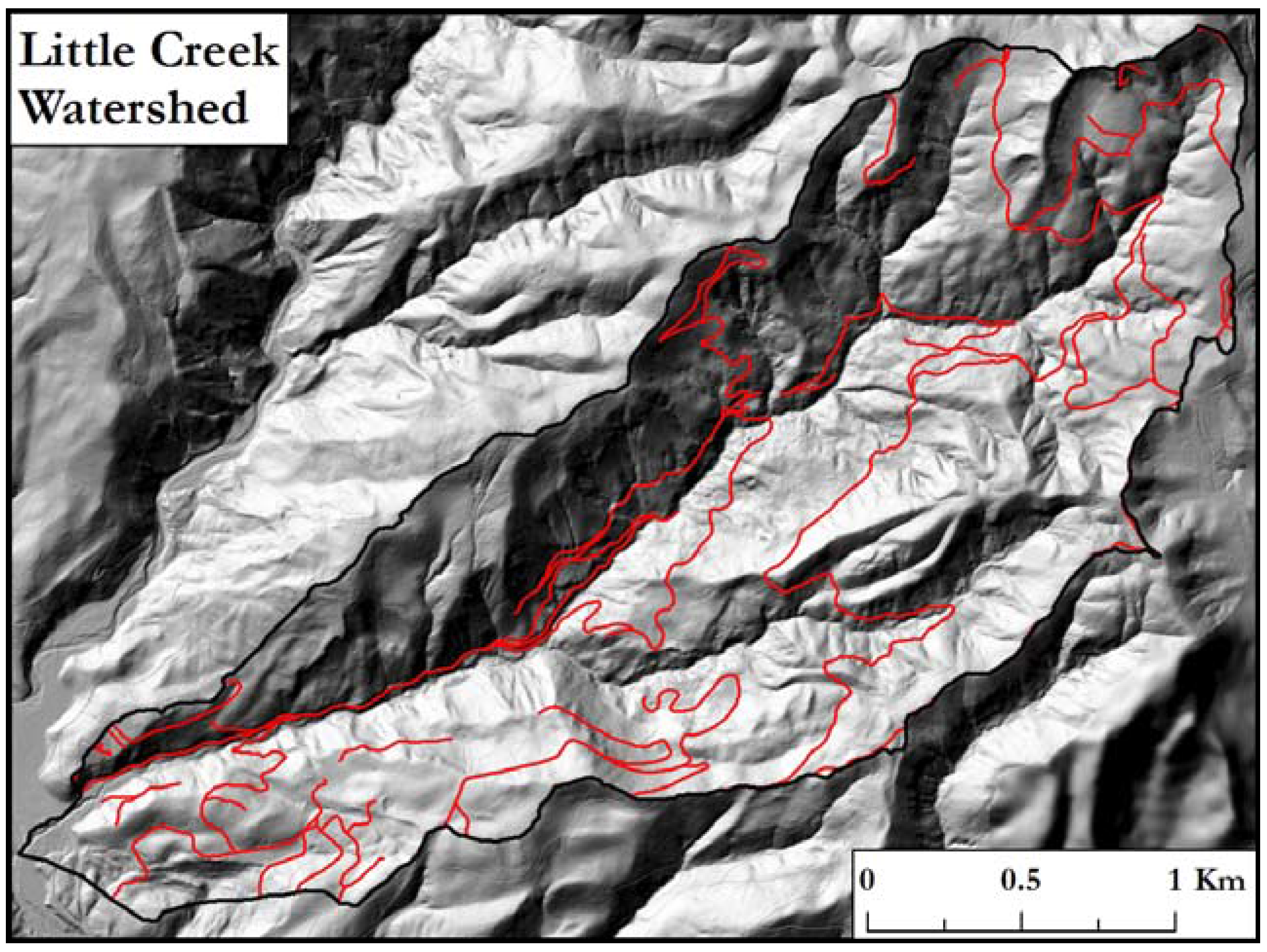
The purpose of this study was to determine the suitability of LiDAR for mapping forest roads in areas of dense forest canopy and steep, complex terrain. Initial objectives of the study included an assessment of the overall quality of LiDAR terrain data collected within the study area. LiDAR quality was evaluated based on the density of ground returns achieved, and the vertical accuracy of the DEM compared to field-surveyed elevation checkpoints. The main objective of the study was to assess the accuracy of road characteristics derived from the LiDAR terrain data, relative to a conventional centerline survey for a four kilometer forest haul road. The limited extent of ground survey data in the study area narrowed the focus of this analysis to the primary forest haul road feature. While this constitutes a relatively small dataset for verification, it serves to demonstrate the suitability of LiDAR terrain data mapping for typical forest road features in steep and forested environments.
Road characteristics were evaluated with the following criteria: (1) completeness; determine the percentage of road length that could be identified and mapped with the LiDAR terrain data, (2) positional accuracy; determine the 95th percentile horizontal distance separating the LiDAR-derived and field-surveyed centerline; (3) road grade; determine the difference in road grade measurements obtained using the LiDAR-derived and field-survey longitudinal profiles, (4) road length; determine the difference in total road length between the LiDAR-derived and field-surveyed centerline.

3.2. Study Area

The geographic setting for this study is the Santa Cruz Mountains on California’s Central Coast. The study site is located 19 km north of the City of Santa Cruz in the Little Creek watershed, a 526-hectare tributary to the Scotts Creek watershed. The lower portion of the Little Creek drainage lies within Swanton Pacific Ranch, a 1,320 hectare educational and research facility owned by the Cal Poly Corporation and managed by Cal Poly State University’s College of Agriculture, Food, and Environmental Sciences.
Topography within the Little Creek watershed is steep and rugged, with elevations ranging from 12 m to 488 m with ground surface slopes exceeding 80% to 100% in some areas. The watershed contains approximately 6.5 km of stream length, for a drainage density of 1.2 km/km2. Streams include first- and second-order streams, as defined by Strahler [44], based on the USGS 1:24,000 topographic map.
Overstory forest canopy in the Little Creek watershed is dominated by second-growth coast redwood Sequoia sempervirens (D. Don) Endl., but also includes components of Douglas-fir Pseudotsuga menziesii (Mirb.) Franco var. menziesii and Tanoak Lithocarpus densiflora (Hook. & Arn.) Rehder. Mature red alder Alnus rubra Bong. is a dominant component of the riparian community and among the few deciduous overstory species in the watershed. The percentage of overstory canopy cover was measured using a vertical densitometer at thirty forest inventory plots throughout the study area. Canopy cover estimates based on these measurements range between 40% and 96%, with an average of 80%.
Figure 1. Little Creek watershed and Swanton Pacific Ranch boundaries shown within the context of the Scotts Creek watershed.
Remotesensing 02 01120 g001

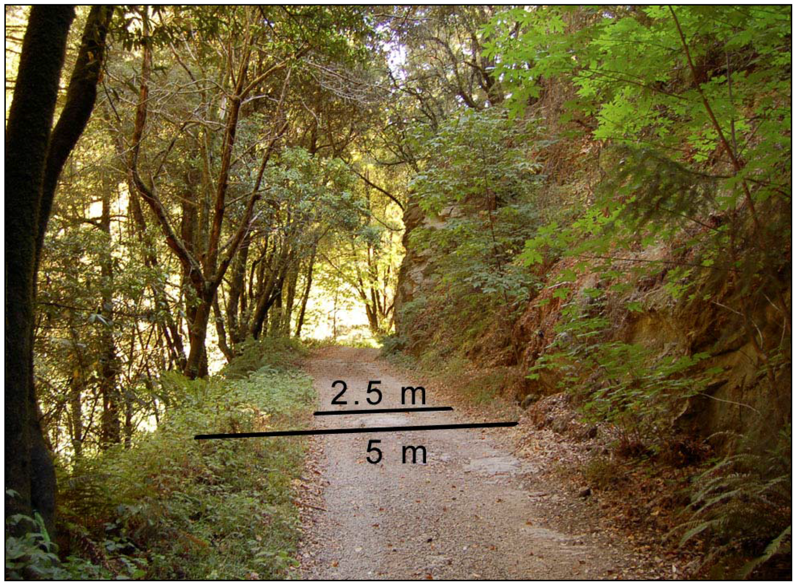
3.3. Target Road Feature

The Little Creek road is a private forest haul road used to access the Little Creek watershed for forest management, field research, and educational activities. Nearly half of the 4 km haul road follows the alignment of a former railroad grade, which was constructed in the early 1900’s. Newer portions of the road were constructed using more modern practices in the late 1980’s. The road segment built on the former railroad grade maintains a low, consistent slope of approximately 7%, originates from the base of the hillslope near the stream channel, and traverses a steep side slope. Road segments constructed using modern practices are located further from the stream channel and encompass road slopes ranging up to 15% to 20% for short distances. Continued use and maintenance of former railroad grades is a common practice in the Santa Cruz Mountains, due to the prevalence of these features and due the high costs and risk of erosion associated with new road construction [45]. The traveled surface width of the Little Creek road varies from 2.5 m to 3.5 m, while the width of the entire road bed measures 5 meters or more (Figure 2).
Figure 2. Little Creek road with dimensions, note the steep cut- and fill-slopes.
Remotesensing 02 01120 g002

4. Methods

4.1. Field Survey Methods

A conventional road centerline survey was conducted to determine centerline location and elevation along the target road feature. The survey was completed by a licensed surveying firm in the spring of 2002, coincident with an earlier LiDAR survey of the study area. The surveyors used high-precision GPS to establish primary control on five nearby High Precision Geodetic Network (HPGN) control points referenced to the North American Datum 1983 with the 1991.35 adjustment. Elevations were referenced to the North American Vertical Datum 1929, and were subsequently adjusted to NAVD 1988 using a upward datum shift of 2.65 ft., based data from the nearest NGS benchmark. A total station was used to determine the horizontal coordinates for 222 points along the road centerline, while conventional leveling with an automatic level was used to determine elevations at 126 of these points. The survey control traverse matched the GPS control by 0.07 m Northing, 0.06 m Easting and 0.07 m vertical. The average distance between points surveyed along the road was 18 m, with curved road segments surveyed at 10 m intervals. The centerline coordinates, elevations, and point descriptions were delivered as layers in a computer-aided design (CAD) file which was later exported to a geodatabase for use in ESRI® ArcGIS™ 9.3 [46].

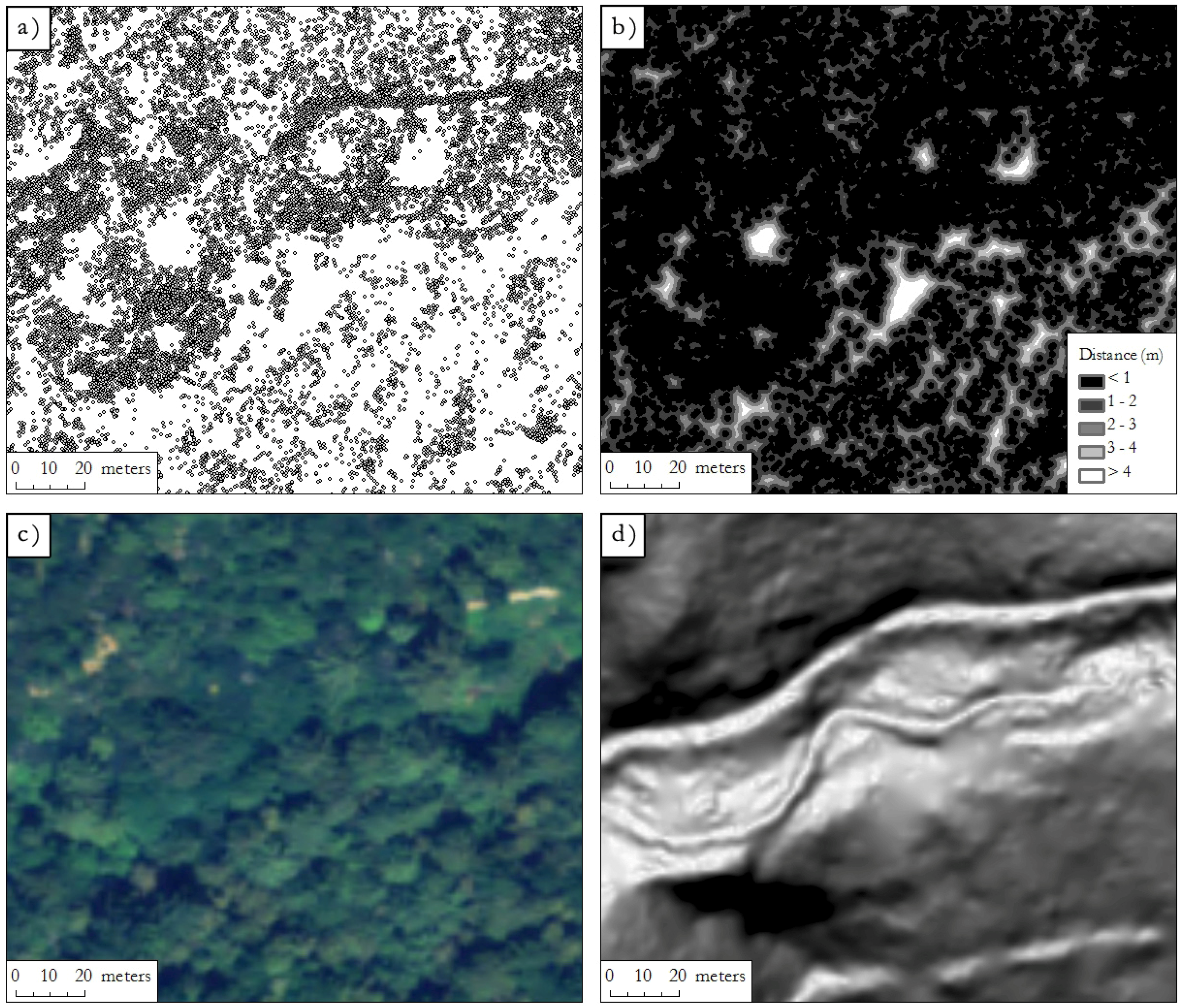
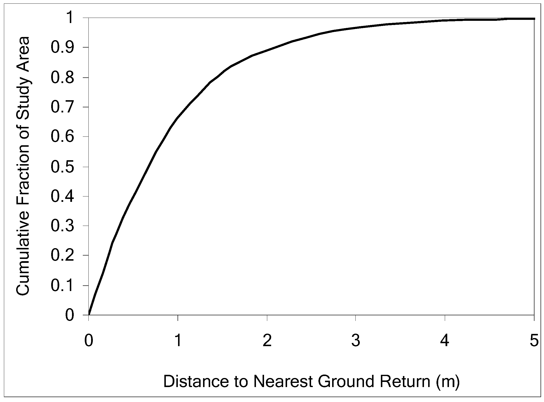
4.2. LiDAR Data Collection and Processing

Airborne LiDAR data were collected by the mapping firm Airborne 1, El Segundo, California, using an Optech ALTM 3100 sensor mounted to a fixed-wing Cessna aircraft. The survey was conducted in February 2008 during leaf-off conditions with the goal of achieving a high density of ground returns. Flight and sensor parameters for the survey are presented in Table 1. LiDAR points were classified by the vendor to identify ground and non-ground returns, while also distinguishing first pulse and last pulse returns. Ground point classification was performed using the commercial software package TerraScan™ (Terrasolid, Ltd.), which employs the adaptive TIN filtering method described by Axelssen [47]. Parameters for ground point classification were selected based on return density and terrain slope within the study area. The resulting bare-earth DEM and derived layers were visually inspected to verify the filtering results. Classified point data were delivered as ASCII text files with X, Y, Z, and intensity values with coordinates in the state plane coordinate system.
Table 1. Flight and sensor parameters.
LiDAR Survey Parameters
Altitude (m AGL)850
Beam divergence (mrad)0.23
Scan angle (º)14
Scan width (m)425
Swath overlap (%)50
Pulse rate (kHz)100
Sampling density (pulses/m2)6
Quality assurance for LiDAR elevations was provided by the vendor using 1,046 Real-Time Kinematic GPS survey points collected on an open highway near the study area. Relative to the GPS elevations, the RMSE for the LiDAR DEM was 0.03 m, with residuals ranging from −0.15 m to 0.07 m. The accuracy assessment was conducted in optimum survey conditions where LIDAR pulses are reflected from smooth terrain surfaces that are free from vegetation and other obstructions.
The quality of the bare-earth DEM and its suitability for mapping terrain features is highly dependent on the density of returns representing the true ground surface. The abundant near-ground vegetation and dense overstory canopy in the study area imposed challenging airborne survey conditions. While the survey provided a high point density (>12 pts/m2), over 94% of these returns were classified as vegetation or non-ground points. Still, the average density of ground returns, determined as the number of ground returns divided by total area, was 0.80 points per square meter, or 1.1 m average point spacing. Within a 15 m buffer of the target road feature, point density was slightly greater at 0.91 points per square meter, or 1.05 m average point spacing. In this study, spacing of ground returns under the forest canopy was highly variable, with open areas receiving a very high point density, while some areas remained completely occluded by vegetation (Figure 3a). An additional measure of ground point spacing was sought to characterize the variation in point spacing.
Figure 3. (a) LiDAR ground returns, (b) Distance to nearest ground return displayed with Euclidian distance grid, (c) 1 m color orthophoto, (d) bare-earth terrain represented with 1 m grayscale slope grid.
Remotesensing 02 01120 g003
The grid-based Euclidean Distance tool in ArcGIS was used to produce a 0.3 m grid where each cell records the distance to the nearest ground return. This approach lends a rapid visualization of point spacing, allowing for quick identification of areas with low point density (Figure 3b). In addition, a cumulative frequency distribution was constructed to display the percentage of the study area occupied by a given distance to the nearest ground return (Figure 4). This figure illustrates that for 65% of the study area, the distance to the nearest ground return was 1 m or less. Interestingly, while large gaps in ground point coverage were found (Figure 3a and Figure 3b), less than 10% of the study area was occupied by gaps where ground points are greater than 2 m distance.
Figure 4. Cumulative frequency distribution for the distance to the nearest ground return.
Remotesensing 02 01120 g004
A 1 m resolution Digital Elevation Model (DEM) was produced from ground returns using the Topo-to-Raster tool in ArcGIS. The interpolation method performed using this tool is based on the ANUDEM method developed by Hutchinson [48], and is specifically designed to model terrain surfaces from irregularly spaced elevation point data. Subsequent layers such as the slope and shaded relief grids were also produced at 1 m resolution using ArcGIS Spatial Analyst. Visually, the quality of bare earth DEM was excellent, with a smooth terrain surface free from aboveground artifacts, while small-scale topographic features such as roads, stream banks, gullies and former landslides were clearly evident.
The Little Creek road was easily identified in the shaded relief image, however, gaps in ground point coverage, particularly along abrupt road edges, degraded the appearance of the road feature (Figure 5a). Upon further investigation, it became apparent that these gaps were not caused by obstructions from dense vegetation, but from the filtering of ground points performed by the vendor. To alleviate this problem, all last return points within a 60 m buffer of the Little Creek road were re-filtered using the multiscale curvature algorithm developed by Evans and Hudak [49]. This method was developed for use in forested areas with complex terrain. Scale and tension parameters of the algorithm and can be adjusted to suit the density of input LiDAR data and topography of the study area. A scale of 2.0 m and tension of 3.0 was selected to retain ground returns located on the abrupt road edges. Newly identified ground returns were added to the original ground returns, increasing the number of ground points by 17.5%. Average point density for this near-road area was improved from 0.91 to 1.08 points per square meter, or to an average point spacing 0.96 m. A new bare-earth DEM was interpolated with inclusion of the added ground points, substantially improving the appearance of steep road edges (Figure 5b). Some manual removal of non-ground returns was employed to limit the introduction of additional noise, particularly in the riparian corridor, though some above-ground artifacts are still apparent (Figure 5b).
Figure 5. (a) Road topography degraded by over-filtering and removal of true ground returns, and (b) improvements in road topography after re-filtering.
Remotesensing 02 01120 g005

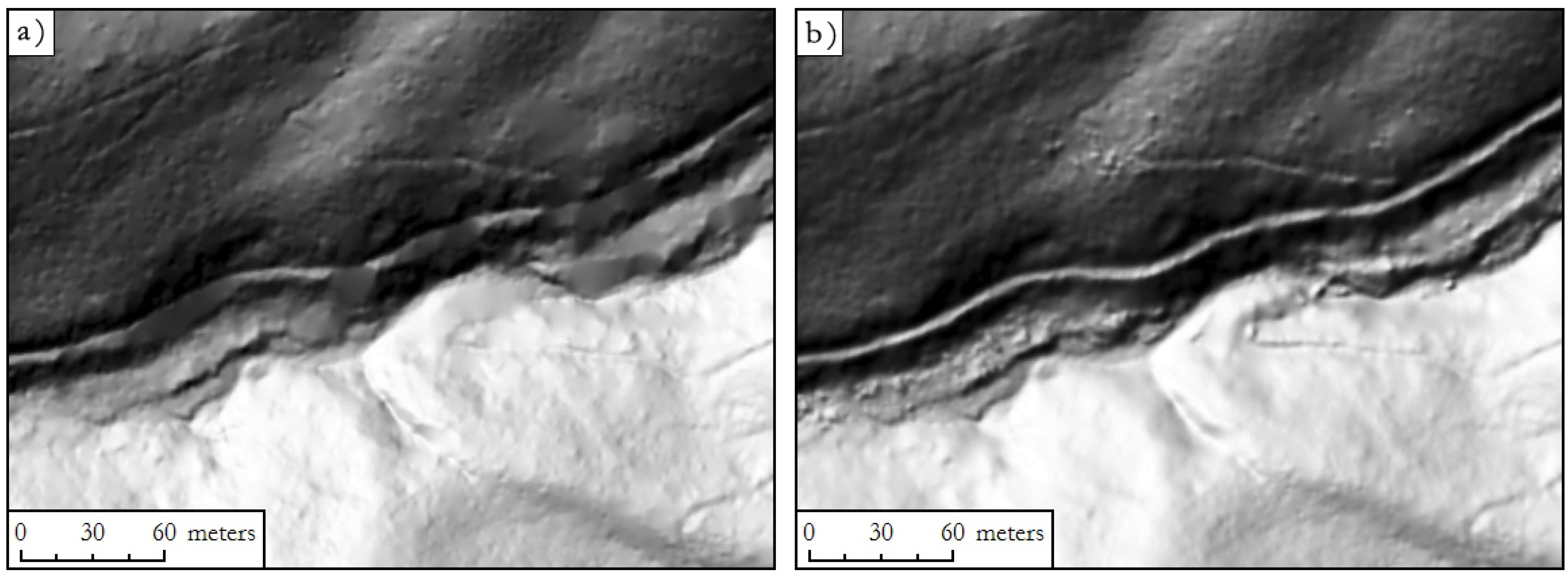
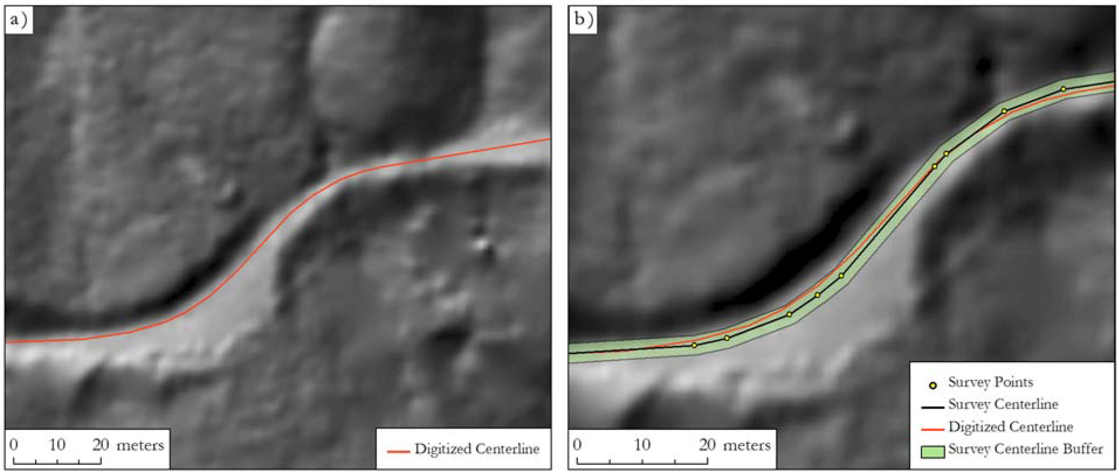
4.3. Road Feature Digitizing

The LiDAR-derived centerline of the Little Creek road was manually digitized in ArcMap through visual interpretation of the shaded relief and slope grids. Topography is relatively easy to interpret from the shaded relief image, however, the drawback is that features are most easily distinguished when illuminated from the side. That is, road features on one aspect may be well defined, while the same feature located on other aspects becomes difficult to distinguish. Here, the slope grid is a valuable complement, because the slope shading is independent of aspect. Using the slope grid can help overcome the difficulties of interpreting multiple shaded relief maps constructed from different sun angles. The slope grid was displayed as a stretched grayscale image with low slopes displayed in white and steep slopes displayed in black (Figure 3b). When viewed this way, the low gradient road surface was displayed in white and is nicely contrasted by steep adjacent road cuts rendered in black [32].
The target road feature was digitized at a map scale ranging from 1:500 to 1:1,000 and was completed within one hour. Upon completion, the digitized line was smoothed using the polynomial approximation with exponential kernel (PAEK) method using the Smooth Line tool in ArcGIS (Figure 6a). The position of the smoothed road was determined using a 15 m moving average and was suitable to smooth the angular appearance of the manually digitized line [46]. This smoothing imparts a minor effect on the horizontal position of the line, though allows the digitized line to match the assumptions of smoothly curving road [50].

4.4. Analysis Methods

LiDAR-derived data were analyzed in three steps. First, elevations from the LiDAR DEM were compared to field-surveyed elevations collected along the road centerline. DEM elevations were extracted for the exact location of the 126 field-surveyed checkpoints. The differences in elevation between the DEM and field-surveyed elevations were used to compute the vertical root mean square error for elevations along the road:
R M S E z = i = 1 n e i 2 n
where ei is the difference between the survey elevation and DEM elevation at point i, and n is the number of elevation checkpoints.
Figure 6. (a) road centerline digitized from LiDAR shaded-relief grid in ESRI ArcMap, (b) field surveyed centerline (black) and digitized centerline (red), note change in scale.
Remotesensing 02 01120 g006
Next, the position of the LiDAR-derived centerline was compared to the field-surveyed centerline location using a simple method presented by Goodchild and Hunter [51]. This approach compares a linear feature of high accuracy to a feature of lower accuracy, and determines the percentage of the low accuracy line that falls within a specified horizontal distance normal to the high accuracy line. The method was used to answer the following question: what percentage of the digitized haul road falls within (x) meters normal to the surveyed road centerline? The width of the buffer needed to achieve a given percentage, 95% of the testline, is used as a measure of overall positional accuracy. An example of this method is presented in Figure 6b where the surveyed centerline is indicated in black, the LiDAR-derived centerline in red, and a buffer of the survey centerline in green, which contains 95% of the LiDAR-derived road length. This method was implemented using a Python script to automate the geoprocessing tasks in ArcGIS. The end result was a buffer around the field-surveyed centerline that enclosed 95% of the length of the LiDAR-derived centerline.
Finally, the LiDAR-derived and field-surveyed longitudinal profiles were plotted and compared visually to examine overall correspondence. For a statistical comparison, a series of 125 road slope measurements were extracted from both the field-measured and LiDAR-derived profiles. A paired t-test was used to determine if there was a statistically-significant difference between the field-surveyed and LiDAR-derived road gradients.

5. Results

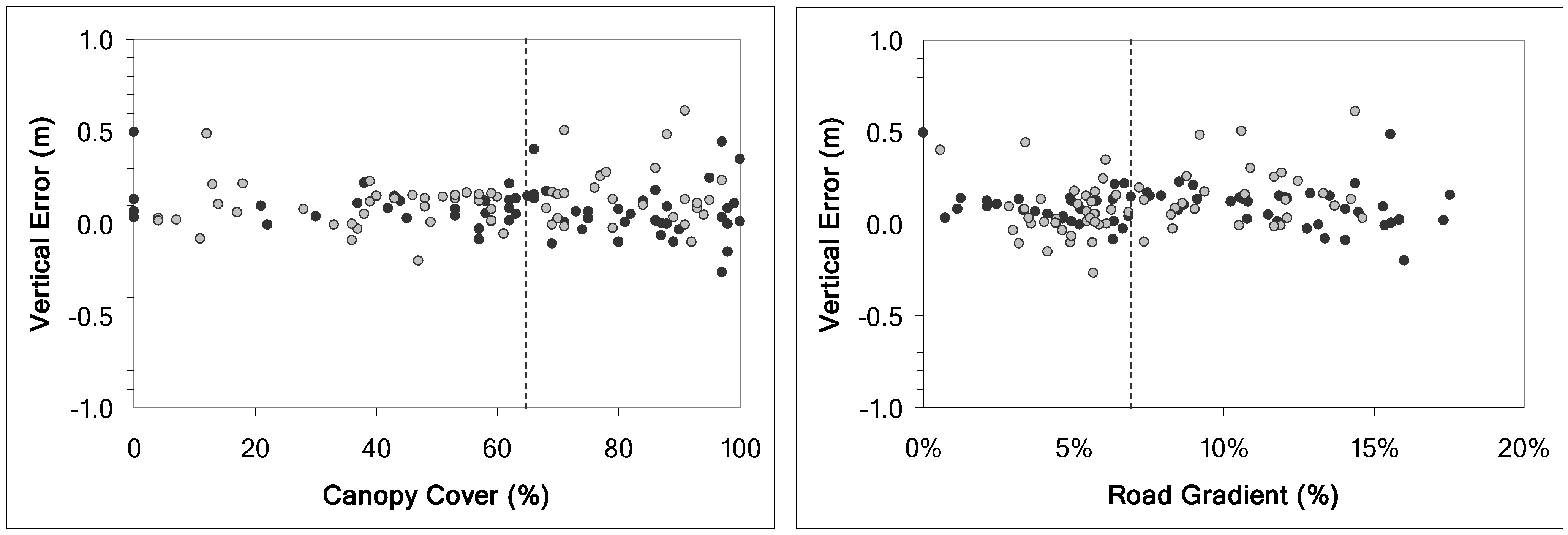
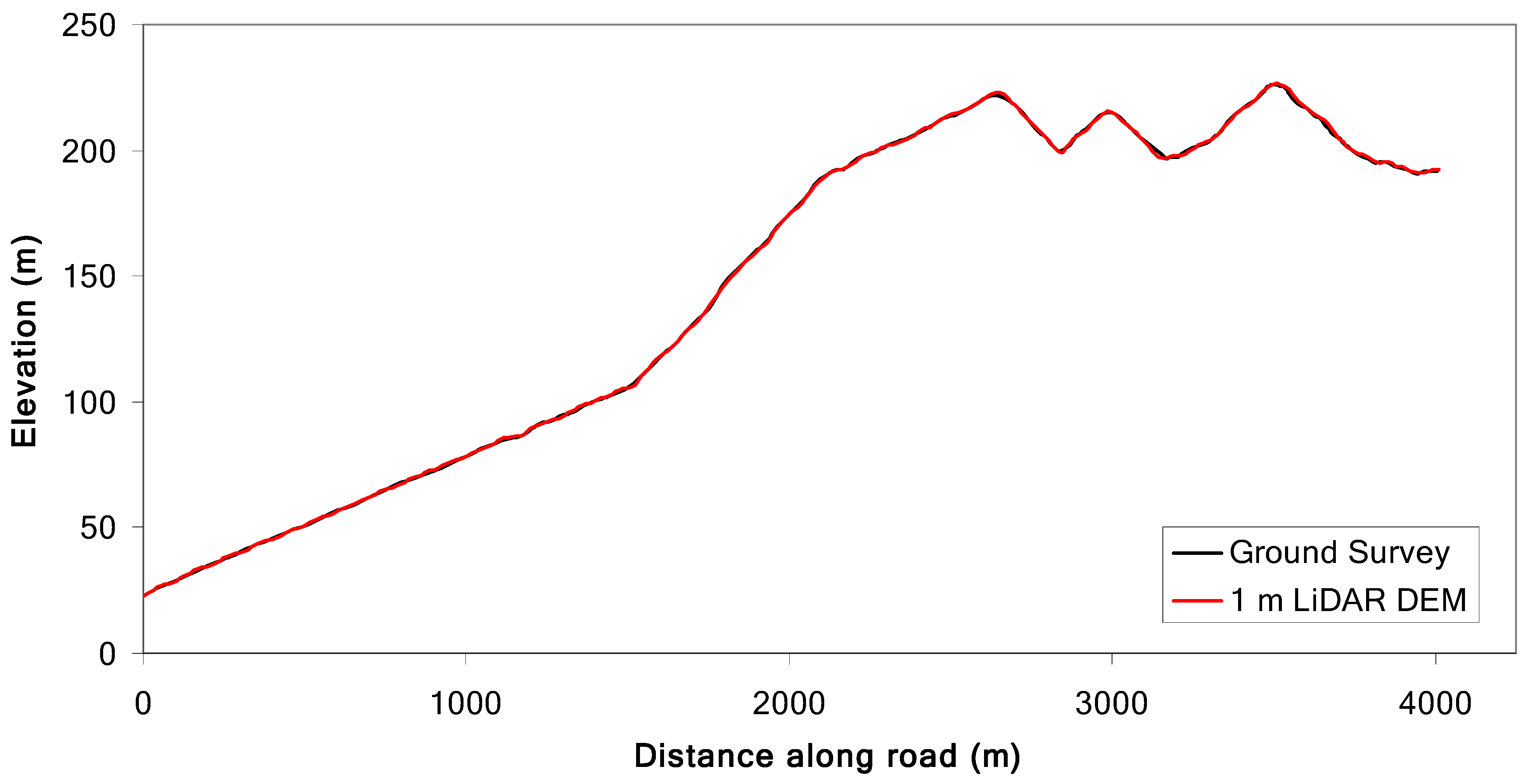
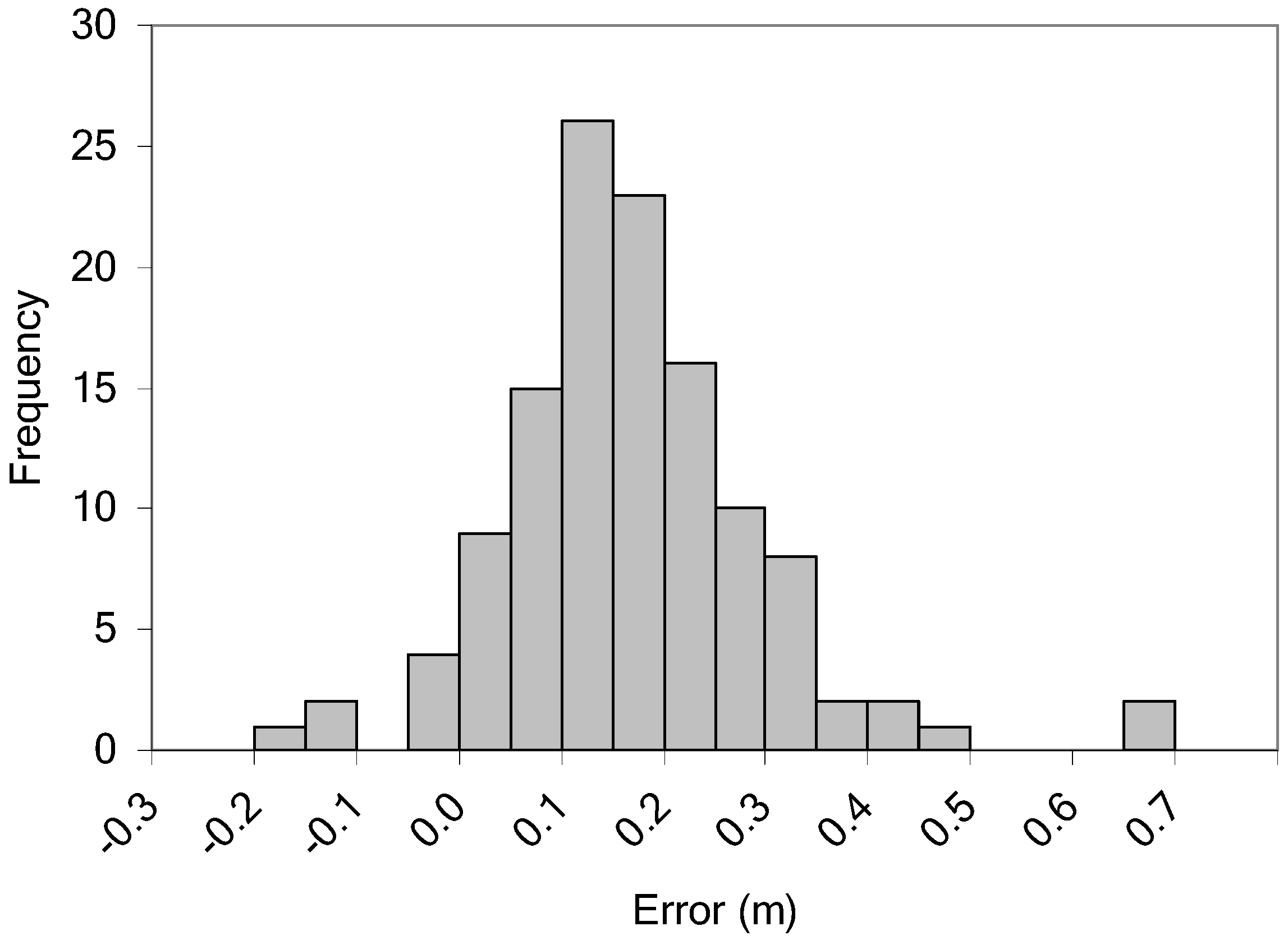
5.1. LiDAR DEM Accuracy

DEM elevations along the Little Creek road corresponded closely to ground survey elevations. The average difference between the LiDAR DEM and survey elevations was 0.10 m ± 0.14 m (mean ± SD). Differences ranged from −0.27 m to 0.61 m. The positive average of 0.10 m and the distribution of errors (Figure 7) indicate an overall bias where DEM elevations were higher on average compared to the field-surveyed elevation. The RMSE for DEM elevations was 0.17 m and falls within the range of vertical accuracies reported for forested areas, given the relatively low terrain slopes of the roadbed [20].
Figure 7. Distribution of LiDAR DEM error computed as DEM elevation—survey elevation at 126 road centerline locations.
Remotesensing 02 01120 g007
The 126 elevation checkpoints along the road centerline were further stratified by road slope and overhead canopy cover to evaluate road steepness and canopy cover effects on vertical error. Two slope classes were established using a 7% slope break, and two canopy cover classes were defined with a 65% cover break. Canopy cover was computed from all returns using the Fusion software developed by McGaughey [52] at the US Forest Service Pacific Northwest Research Station, and was defined as the ratio of vegetation returns (>2 m above the ground), versus the total number of returns within a 5 m pixel. The stratification of checkpoints resulted in a roughly even number of observations per group (Table 2). The mean and standard deviation of vertical error for the groups are presented in Table 3.
Table 2. Number of observations per group.
Low CoverHigh CoverOverall
Low Slope283563
High Slope362763
Overall6462126
Table 3. Mean and standard deviation for signed vertical error (m) for elevation checkpoints in four slope and canopy cover groups.
Low Cover High Cover Overall
MeanSD MeanSD MeanSD
Low Slope0.100.10 0.060.15 0.080.13
High Slope0.090.12 0.160.17 0.120.15
Overall0.090.110.110.160.100.14
As expected, the magnitude of vertical error appeared slightly greater for areas of higher slope and overhead canopy cover, however the differences were relatively small. Evaluated separately, a t-test between low slope and high slope groups indicated a difference in mean error of 0.04 m, though the difference was not significant at a 95% confidence level. Differences in mean error between low canopy cover and high canopy cover groups also failed to produce a significant result. Evaluated together using tukey’s pairwise comparison (family error rate 0.05), only the high slope, high cover group demonstrated a significant difference to any other group, the low slope and high cover group. Figure 8 displays the vertical errors plotted by increasing canopy cover (left) and increasing road grade (right). Again, only slight differences in vertical error are observed across the x-axis in each graph. If anything, higher magnitude errors appear as grey points on the right side of each graph, indicating that high magnitude errors were observed in areas of both high slope and high cover.
Figure 8. Left: DEM elevation error versus canopy cover. Grey points denote errors within high slope group. Right: DEM elevation error versus road gradient. Grey points denote errors within the high canopy cover group. Dashed vertical line denotes division between groups.
Remotesensing 02 01120 g008

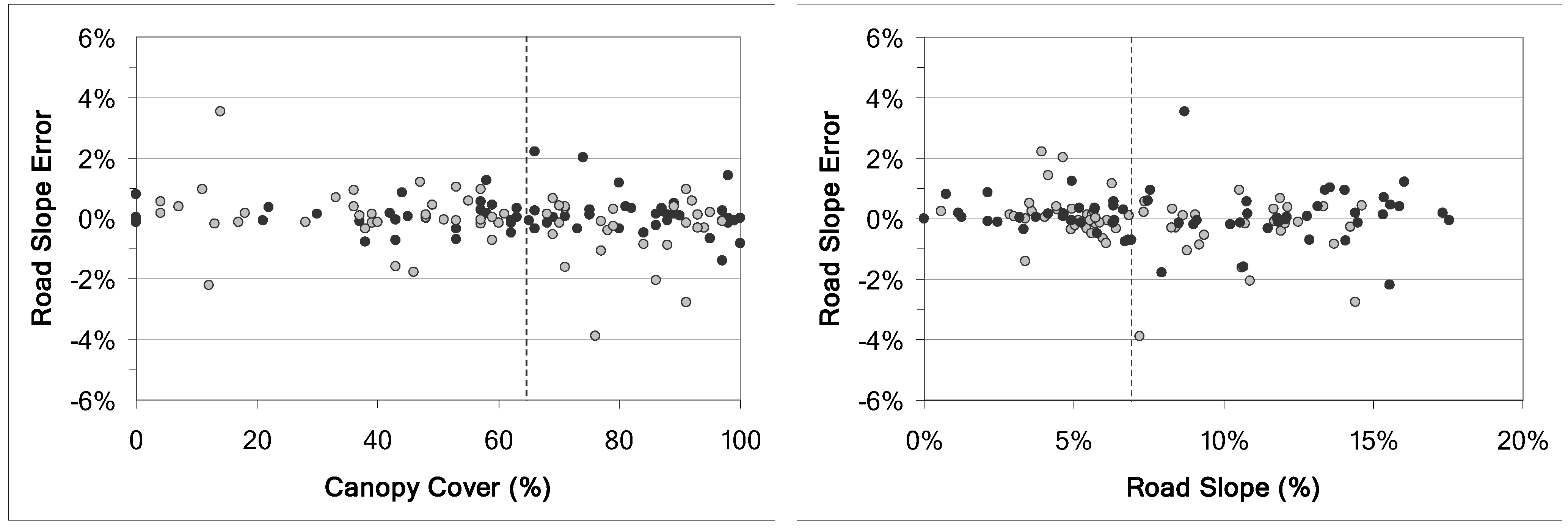
5.2. LiDAR-Derived Feature Accuracy

An extensive network of current forest roads, historic roads, skid trails, and other recreational trails were visible within the Little Creek watershed. A total of 30 kilometers of road and trail features were digitized, though only the Little Creek road was used in the accuracy assessment (Figure 9). In terms of completeness, the full length (100%) of the target road feature was clearly visible in the 1 m resolution shaded-relief and slope grids. By comparison, only 15% of the road feature was directly visible from a 1 m color orthophoto.
Figure 9. LiDAR-derived roads in the Little Creek watershed.
Remotesensing 02 01120 g009
Road edges were well-defined in the LiDAR-derived layers and enabled an accurate digitizing of centerline location. Ninety-five percent of the LiDAR-derived road (3.8 km of 4 km) was digitized within 1.5 m normal to the field-surveyed centerline (Figure 6). The remaining five percent of the road length (0.2 km) was located further than 1.5 m from the surveyed centerline, though the maximum separation between the field-surveyed and digitized centerline did not exceed 2.0 m.
Differences between field-surveyed and LiDAR-derived slope from 125 road segments were compared using a paired t-test. A p-value of 0.972 indicated that the differences in road slope were not significantly different from zero. The mean absolute difference (MAD) in measured road slope over all 125 segments was 0.53%. A maximum slope error of nearly 3.5% was observed in two locations. Given that DEM elevation errors for these points were significantly different only at locations of high road slope and high canopy cover, it was expected that slope measurement were similarly affected. Indeed, analysis of variance for signed slope errors stratified by road slope and canopy cover indicated that higher-magnitude slope errors occurred in areas of high slope and high canopy cover, though these differences were not statistically significant. Mean and standard deviation of slope errors are presented in Table 4.
Table 4. Mean and standard deviation for signed slope error (%) for road segments in four slope and canopy cover groups.
Low Cover High Cover Overall
MeanSD MeanSD MeanSD
Low Slope0.070.47 0.120.94 0.110.16
High Slope0.150.69 −0.401.09 −0.111.03
Overall0.100.77 −0.090.92 0.000.09
LiDAR-derived slope errors are plotted by canopy cover and by road gradient in Figure 10. Slope errors display little discernable pattern across the x-axis. Slope errors plotted by road grade did exhibit a slight tendency to under-predict surveyed slope at higher gradients, similar results were reported by Hodgson et al. [53].
Figure 10. Left: Slope measurement error versus canopy cover. Gray points denote errors within the high road slope group. Right: Slope measurement error versus road gradient. Gray points denote errors within the high canopy cover group. Dashed vertical line denotes division between groups.
Remotesensing 02 01120 g010
A highly reliable longitudinal profile (Figure 11) was obtained given the accuracy of the DEM elevations and LiDAR-derived road position. The total length of the LiDAR-derived centerline was 4,012.9 m, slightly longer than the field-surveyed centerline. The 6.4 m difference can be expressed as a 0.2% difference or as a ratio of error of 1:600. That is, for every 600 m of true road length, one meter of error is encountered in the digitized road length.
Figure 11. Longitudinal profiles derived from ground survey and LiDAR data.
Remotesensing 02 01120 g011

6. Discussion

Forest road information generated from LiDAR can serve a variety of purposes for resource managers. Producing a thorough and updated map of road features is among the most valuable and easily attained products of LiDAR data analysis. In this study, a substantial number of current and former roads, skid trails, and other recreational trails were mapped. In general, all major forest roads suitable for vehicle traffic were identified, though only the target road feature was verified using ground survey data. Some skid trails, particularly those that do not have a pronounced topographic cross-section, were difficult to identify using LiDAR surface grids. Road features mapped using LiDAR were typically not visible using the traditional orthophoto. Only 15% of the target road feature was directly visible from the 1 m color orthophoto.
From an operational standpoint, particularly in the field of resource management, road extraction largely remains a manual process, despite the growing number of automated and semi-automated software tools [54]. In this study, manual digitizing provided a simple, effective. and relatively efficient method for mapping road features, though there are some disadvantages. Due to the level of user interpretation required in manual digitizing, additional errors would be expected from examining multiple trials from different digitizers. The level of positional error associated with manual road extraction among different individuals will vary depending a number of factors, but has been reported to vary by approximately 3 meters between different individuals [54]. Errors introduced through user interpretation and digitizing style can be reduced through focused training [50]. Finally, if mapping were conducted over larger extents, hundreds to thousands of square kilometers, automated and semi-automated road extractions techniques may offer substantial time-savings, though these methods also require additional training to achieve improvements in efficiency [54].
For forest management, access to high-resolution terrain data can provide better agreement between initial office-based plans and true field conditions. With LiDAR-derived background layers, foresters can identify important topographic conditions before entering the field, aiding the initial planning and harvest layout. Mapping remnant and previously unknown road features may also allow existing infrastructure to be used for timber harvest operations or for wildland fire preparedness. Identifying road infrastructure is essential for wildland fire planning and suppression measures. In the Santa Cruz Mountains, large and small private landowners maintain extensive road networks, though these are generally not collectively organized for purposes of watershed assessment or fire planning. The 2009 Lockheed Fire, which burned over 7,800 acres including 92% of the Little Creek watershed, provided a dramatic, local example of the need to coordinate data regarding resources and infrastructure among landowners and wildland firefighters.
In addition to providing complete road features, road characteristics measured using LiDAR and GIS methods were highly accurate. The ±1.5 m positional accuracy for road features is a substantial improvement to the ±12 m accuracy of road features appearing on the USGS 1:24,000 topographic maps [55]. A similar level of positional accuracy of one to two meters for an extracted road centerline was reported by Rieger et al. [32]. The level of positional accuracy needed for GIS datasets varies substantially with their intended uses. For analysis conducted at the scale of this study, positional accuracy affects the accuracy of other attributes, such as road length and gradient. A simple criterion for horizontal accuracy in this study was that the digitized centerline must lie within the width of the actual road bed. Elevations for the road profile were extracted from the DEM along the road centerline and these elevations must represent the elevation of the road bed rather than the elevation of the adjacent side slopes. The maximum distance between the field-survey centerline and the digitized line was 2.0 m and was essentially one-half of the width of the Little Creek road.
Road gradient is a key parameter used to estimate rates of road erosion [2]. LiDAR-derived road slope measurements compared to surveyed slopes with an overall mean absolute difference of 0.53%. In addition, the accuracy of road slope measurements was not significantly affected by increases in overhead canopy cover or road slope. A relatively small sample size was used for this analysis, though results fall in-line with previously reported values for forested areas [20,53]. While road grade measurements may be used with confidence, a host of other road characteristics are typically needed to accurately estimate road erosion. Inventory data, such as road surface material, evidence of splash, sheet, and rill erosion, amount of traffic, and the specific location of road drainage features (waterbars, rolling dips, or cross drains) are usually collected in the field [12] and are not likely to be reliably extracted from LiDAR data. Similar needs to verify field conditions were identified by Krogstad and Schiess [30] when planning the alignment of new forest roads. Important field conditions such as saturated soils or exposed bedrock cannot be identified from the LiDAR-derived products. Field observations and verification and remain essential for many management activities. For these reasons, LiDAR data analysis is not intended to wholly replace field-based surveys or detailed road inventories, rather, it serves to support these activities by providing the background topography, layout, and fundamental measurements of the road system.
Access to high resolution LiDAR terrain data is likely to expand rapidly in the coming decade through collaborative efforts of regional consortia and county, state, and nationwide mapping initiatives (http://lidar.cr.usgs.gov/). Efficient mapping techniques must be developed to take full advantage of the scale and detail of these improved datasets. Automated or semi-automated road extraction techniques are important areas for future research. Of the available commercial software, RoadTracker™ distributed by Overwatch Geospatial (http://geospatial.overwatch.com/) is designed to extract road features from imagery, though has yet to be applied to LiDAR-derived imagery in forested areas. Likewise, methods for extracting other road parameters such as cross-sectional geometry, cut slope height, and estimating the volume of sediment for fill slopes and stream crossings are worth further investigation.

7. Conclusion

High quality LiDAR-derived data were produced in the challenging survey conditions of the densely forested and rugged Santa Cruz Mountains, CA, USA. While over 94% of LiDAR returns were filtered as vegetation points, the remaining ground points supported a 1 m resolution DEM. The shaded-relief and slope layers derived from the bare-earth DEM highlighted forest road features that could not be mapped though traditional aerial photography. Over 30 km of forest roads and trail features were mapped within the study area. The ability to identify and map road networks in forested areas was substantially improved compared to traditional data sources. In this study, a high level of positional accuracy was achieved for the LiDAR-derived road feature. Ninety-five percent of the digitized road length was located within 1.5 m normal to the conventional field-surveyed centerline. This level of positional accuracy permitted highly reliable measurement of other road characteristics, with total road length measured to within 0.2% and road segment slopes measured with a mean absolute difference of 0.53%.
Road position, length, and gradient are important inventory parameters for forest management and watershed assessment. These measurements can be obtained accurately and efficiently using high-resolution LiDAR data, reducing the need for field-based surveys for these basic parameters. Greater opportunities now exist for broad-scale analyses that incorporate thorough and accurate measurements of forest road systems. LiDAR-derived road data can address gaps that exist in current data sources, especially for forested areas, and represent a valuable tool to assess forest roads at scales not previously feasible.

Acknowledgements

Partial funding for this research was provided through the CSU Agricultural Research Initiative with support from Cal Poly Swanton Pacific Ranch. The authors would like to thank the anonymous reviewers for their contributions to this manuscript.

References and Notes

  1. Montgomery, D.R. Road surface drainage, channel initiation, and slope instability. Water Resour. Res. 1994, 30, 1925–1932. [Google Scholar] [CrossRef]
  2. Luce, C.H.; Black, T.A. Sediment production from forest roads in western Oregon. Water Resour. Res. 1999, 35, 2561–2570. [Google Scholar] [CrossRef]
  3. Bilby, R.E.; Sullivan, K.; Duncan, S.H. The generation and fate of road-surface sediment in forested watersheds in Southwestern Washington. Forest Sci. 1989, 35, 453–468. [Google Scholar]
  4. Frissell, C.A. Topology of extinction and endangerment of native fishes in the Pacific Northwest and California (USA). Conserv. Biol. 1993, 7, 342–354. [Google Scholar] [CrossRef]
  5. USDA Forest Service. Roads Analysis: Informing Decisions about Managing the National Forest Transportation System; USDA Forest Service: Washington, DC, USA, 1999.
  6. CDF. California Forest Practice Rules; California Department of Forestry and Fire Protection: Sacramento, CA, USA, 2009.
  7. Jones, J.A.; Swanson, F.J.; Wemple, B.C.; Snyder, K.U. Effects of roads on hydrology, geomorphology, and disturbance patches in stream networks. Conserv. Biol. 1999, 14, 76–85. [Google Scholar] [CrossRef]
  8. McGurk, B.J.; Fong, D.R. Equivalent roaded area as a measure of cumulative effect of logging. Environmen. Manage. 1995, 19, 609–621. [Google Scholar]
  9. Dubé, K.V.; Megahan, W.F.; McCalmon, M. Washington Road Surface Erosion Model; Washington Department of Natural Resources: Olympia, WA, USA, 2004.
  10. Dubé, K.; McCalmon, M. Technical Documentation for Sedmodl, Version 2.0 Road Erosion/Delivery Model. 2004. Available online: http://www.ncasi.org/support/downloads (accessed on 7 December 2009).
  11. Brooks, E.S.; Boll, J.; Elliot, W.J.; Tom, D. Global positioning system/GIS-based approach for modeling erosion from large road networks. J. Hydrol. Eng. 2006, 11, 418–426. [Google Scholar] [CrossRef]
  12. Prasad, A.; Tarboton, D.G.; Luce, C.H.; Black, T.A. A GIS tool to analyze forest road sediment production and stream impacts. In Proceedings of the 25th ESRI Users Conference, San Diego, CA, USA, July 2005.
  13. Jazouli, R.; Verbyla, D.L.; Murphy, D.L. Evaluation of spot panchromatic digital imagery for updating road locations in a harvested forest area. Photogramm. Eng. Remote Sens. 1994, 60, 1449–1452. [Google Scholar]
  14. Gucinski, H.; Furniss, M.J.; Ziemer, R.R.; Brookes, M.H. Forest Roads: A Synthesis of Scientific Information; PNW-GTR-509; USDA Forest Service, Pacific Northwest Research Station: Corvallis, OR, USA, 2001.
  15. Coghlan, G.; Sowa, R. National Forest Road System and Use (Draft Report); USDA Forest Service: Washington, DC, USA, 1998.
  16. Keane, R.E.; Long, D.G.; Menakis, J.P.; Hann, W.J.; Bevins, C.D. Simulating Coarse Scale Vegetation Dynamics Using the Columbia River Basin Succession Model-CRBSUM; USDA Forest Service, Intermountain Research Station: Ogden, UT, USA, 1996.
  17. Lee, D.C.; Scedell, J.R.; Thurow, R.F.; Williams, J.E.; Burns, D.; Clayton, J.; Decker, L.; Gresswell, R.; House, R.; Howell, P.; Lee, K.M.; Overton, C.T.; Perkinson, D.; Tu, K.; Van Eimeren, P. Broadscale assessment of aquatic species and habitats. In The Interior Columbia Basin Ecosystem Management Project: Scientific Assessment; Quigley, T.M., Ed.; U.S. Department of Agriculture, Forest Service, Pacific Northwest Research Station: Portland, OR, USA, 1997; pp. 1057–1713. [Google Scholar]
  18. Forman, R.T.; Sperling, T.D.; Bissonette, J.A.; Clevenger, A.P.; Cutshall, C.D.; Dale, V.H.; Fahrig, L.; France, R.; Goldman, C.R.; Heanue, K.; Jones, J.A.; Swanson, F.J.; Turrentine, T.; Winter, T.C. Road ecology: Science and Solutions; Island Press: Washington, DC, USA, 2003. [Google Scholar]
  19. Menning, K.M.; Erman, D.C.; Johnson, K.N.; Sessions, J. Modeling Aquatic and Riparian Systems, Assessing Cumulative Watershed Effects, and Limiting Watershed Disturbance; Sierra Nevada Ecosystem Project: Final Report to Congress, Addendum; University of California, Centers for Water and Wildland Resources: Davis, CL, USA, 1996; pp. 33–51. [Google Scholar]
  20. Reutebuch, S.E.; McGaughey, R.J.; Andersen, H.-E.; Carson, W. Accuracy of a high-resolution LiDAR terrain model under a conifer forest canopy. Can. J. For. Res. 2003, 29, 527–535. [Google Scholar] [CrossRef]
  21. Evans, J.; Hudak, A.; Faux, R.; Smith, A.M.S. Discrete return LiDAR in natural resources: recommendations for project planning, data processing, and deliverables. Remote Sens. 2009, 1, 776–794. [Google Scholar] [CrossRef]
  22. Shrestha, R.L.; Carter, W.E.; Lee, M.; Finer, P.; Satori, M. Airborne laser swath mapping: Accuracy assessment for surveying and mapping applications. Surveying and Land Information Systems 1999, 59, 83–94. [Google Scholar]
  23. Hudak, A.T.; Evans, J.S.; Smith, A.M.S. LiDAR utility for natural resource managers. Remote Sensing 2009, 1, 934–951. [Google Scholar] [CrossRef]
  24. Reutebuch, S.E.; Andersen, H.-E.; McGaughey, R.J. Light detection and ranging (LiDAR): An emerging tool for multiple resource inventory. J. Forest. 2005, 103, 286–292. [Google Scholar]
  25. Falkowski, M.J.; Evans, J.S.; Martinuzzi, S.; Gessler, P.E.; Hudak, A.T. Characterizing forest succession with LiDAR data: An evaluation for the Inland Northwest, USA. Remote Sens. Environ. 2009, 113, 946–956. [Google Scholar] [CrossRef]
  26. Kraus, K.; Pfeifer, N. Determination of terrain models in wooded areas with airborne laser scanner data. J. Photogramm. Remote Sens. 1998, 53, 193–203. [Google Scholar] [CrossRef]
  27. Schulz, W.H. Landslides susceptibility revealed by LiDAR imagery and historical records, Seattle, Washington. Eng. Geol. 2007, 89, 67–87. [Google Scholar] [CrossRef]
  28. James, L.A.; Watson, D.G.; Hansen, W.F. Using LiDAR data to map gullies and headwater streams under forest canopy: South Carolina, USA. Catena 2007, 71, 132–144. [Google Scholar] [CrossRef]
  29. Crow, P.; Benham, S.; Devereux, B.J.; Amable, G.S. Woodland vegetation and its implications for archaeological survey using LiDAR. Forestry 2007, 80, 241–252. [Google Scholar] [CrossRef]
  30. Krogstad, F.; Schiess, P. The allure and pitfalls of using LiDAR topography in harvest and road design. In Proceedings of The International Mountain Logging Conference, Vancouver, BC, Canada; 2004. [Google Scholar]
  31. Aruga, K.; Sessions, J.; Miyata, E.S. Forest road design with soil sediment evaluation using a high resolution DEM. J. For. Res. 2005, 10, 471–479. [Google Scholar] [CrossRef]
  32. Rieger, W.; Kerschner, M.; Reiter, T.; Rottensteiner, F. Roads and buildings from laser scanner data within a forest enterprise. In Proceedings of the ISPRS Workshop “Mapping Surface Structure And Topography By Airborne And Spaceborne Lasers”, La Jolla, CA, USA.International Archives of Photogrammetry and Remote Sensing; Csatho, B.M. (Ed.) 1999; Volume XXXII, pp. 185–191.
  33. David, N.; Mallet, C.; Pons, T.; Chauve, A.; Bretar, F. Pathway detection and geometrical description from ALS data in forested mountainous area. In Proceedings of Laser Scanning 2009, Paris, France; Bretar, F., Pierrot-Deseilligny, M., Vosselman, G., Eds.; 2009; Volume XXXVIII. [Google Scholar]
  34. Quackenbush, L. A review of techniques for extracting linear features from imagery. Photogramm. Eng. Remote Sens. 2004, 70, 1383–1392. [Google Scholar] [CrossRef]
  35. Clode, S.; Rottensteiner, F.; Kootsookos, P.; Zelniker, E. Detection and vectorization of roads from LiDAR data. Photogramm. Eng. Remote Sens. 2007, 73, 517–536. [Google Scholar] [CrossRef]
  36. Auclair-Fortierm, M.-F.; Ziou, D.; Armenakis, C.; Wang, S. Survey of Work on Road Extraction in Aerial and Satellite Images; Tech. Rep. TR-247; Department of Mathematics and Computer Science, University of Sherbrooke: Québec, Canada, 2000. [Google Scholar]
  37. Clode, S.P.; Zelniker, E.E.; Kootsookos, P.J.; Clarkson, I.V.L. A phase coded disk approach to thick curvilinear line detection. In Proceedings of the XII European Signal Processing Conference, Vienna, Austria, September 2004; pp. 1147–1150.
  38. Alharthy, A.; Bethel, J. Automated road extraction from LiDAR data. In Proceedings of American Society of Photogrammetry and Remote Sensing Annual Conference, Anchorage, AK, USA, 2004.
  39. Asner, G.P.; Keller, M.; Pereira, R.; Zweede, J. Remote sensing of selective logging in Amazonia assessing limitations based on detailed field observations, Landsat ETM+, and textural analysis. Remote Sens. Environ. 2002, 80, 483–496. [Google Scholar] [CrossRef]
  40. Lee, H.; Slatton, K.C.; Jhee, H. Detecting forest trails occluded by dense canopies using alsm data. In Proceedings of the Geoscience and Remote Sensing Symposium, Seoul, South Korea, July 2005.
  41. Shamayleh, H.; Khattak, A. Utilization of LiDAR technology for highway inventory. In Proceedings of the 2003 Mid-Continent Transportation Research Symposium, Ames, IA, USA, August 2003.
  42. Souleyrette, R.; Hallmark, S.; Pattnaik, S.; O’Brien, M.; Veneziano, D. Grade and cross slope estimation from LiDAR-based surface models. In Application of Advanced Remote Sensing Technology to Asset Management; Hallmark, S., Ed.; Midwest Transportation Consortium: Ames, IA, USA, 2003. [Google Scholar]
  43. Carson, W.W.; Andersen, H.-E.; Reutebuch, S.E.; McGaughey, R.J. LiDAR applications in forestry—An overview. In Proceedings of the American Society of Photogrammetry and Remote Sensing Annual Conference, Denver, CO, USA, May 2004.
  44. Strahler, A. Quantitative geomorphology of drainage basins and channel networks. In Handbook of Applied Hydrology; Chow, V.T., Ed.; McGraw-Hill: New York, NY, USA, 1964. [Google Scholar]
  45. Weaver, W.E.; Hagans, D.K. Handbook for Forest and Ranch Roads; Pacific Watershed Associates: Arcata, CA, USA, 1994. [Google Scholar]
  46. ESRI. ArcGIS; Environmental Systems Research Institute: Redlands, CA, USA, 2008. [Google Scholar]
  47. Axelsson, P. DEM generation from laser scanner data using adaptive TIN models. In Proceedings of XIXth ISPRS Congress, Amsterdam, The Netherlands; 2000. [Google Scholar]International Archives of Photogrammetry and Remote Sensing; 2000; Volume XXXIII, Part B4.
  48. Hutchinson, M.F. A new procedure for gridding elevation and stream line data with automatic removal of spurious pits. J. Hydrol. 1989, 106, 211–232. [Google Scholar] [CrossRef]
  49. Evans, J.S.; Hudak, T. A multiscale curvature algorithm for classifying discrete return LiDAR in forested environments. IEEE Trans.Geosci. Remote Sens. 2007, 45, 1029–1038. [Google Scholar] [CrossRef]
  50. Jenks, G. Lines, computers, and human frailties. Ann. Assn. Amer. Geogr. 1981, 71, 1–10. [Google Scholar] [CrossRef]
  51. Goodchild, M.F.; Hunter, G.J. A simple positional accuracy measure for linear features. Int. J. Geogr. Inf. Sci. 1997, 11, 299–306. [Google Scholar] [CrossRef]
  52. McGauhey, R.J. FUSION/LDV: Software for LiDAR Data Analysis and Visualization; USDA Forest Service, Pacific Northwest Research Station: Seattle, WA, USA, 2009.
  53. Hodgson, M.E.; Jensen, J.; Raber, G.; Tullis, J.; Davis, B.A.; Thompson, G.; Schuckman, K. An Evaluation of LiDAR-derived elevation and terrain slope in leaf-off conditions. Photogramm. Eng. Remote Sens. 2005, 71, 817–823. [Google Scholar] [CrossRef]
  54. Doucette, P.; Grodecki, J.; Clelland, R.; Hsu, A.; Nolting, J.; Malitz, S.; Kavanagh, C.; Barton, S.; Tang, M. Evaluating automated road extraction in different operational modes. In Algorithms and Technologies for Multispectral, Hyperspectral, and Ultraspectral Imagery XV; Shen, S.S., Lewis, P.E., Eds.; SPIE: Bellingham, WA, USA, 2009; Proceedings of SPIE Series; Volume 7334. [Google Scholar]
  55. US Bureau of the Budget. United States National Map Accuracy Standards; US Bureau of the Budget: Washington, DC, USA, 1947.

