Individual Tree Species Classification by Illuminated—Shaded Area Separation


Abstract
:
1. Introduction
1.1. Use of Species Classification in Forest Management
1.2. LIDAR and Aerial Image Based Methods
1.3. Methodology Comparison Studies
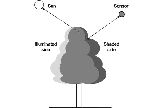
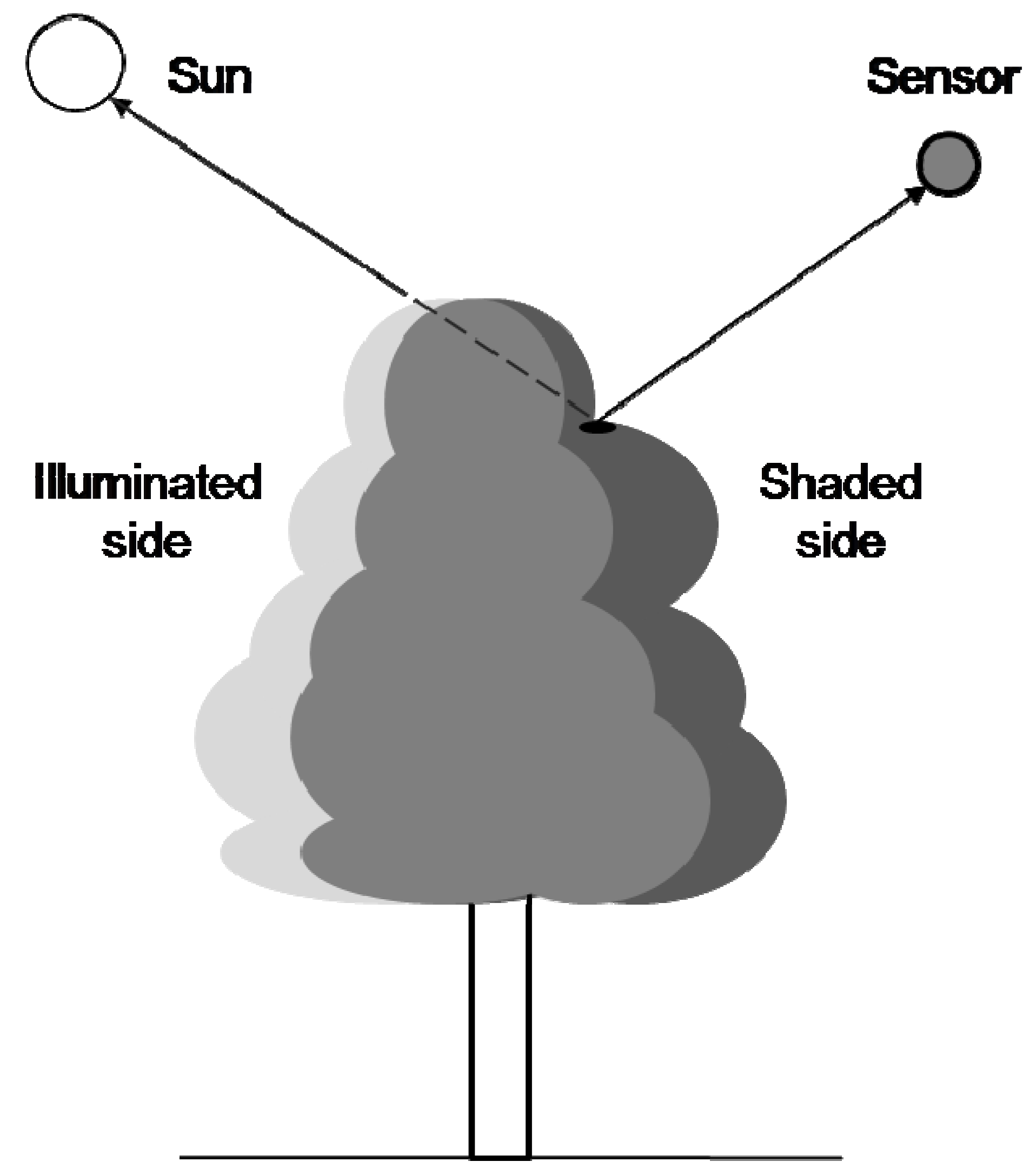
1.4. Tree Canopy Division into Illuminated and Shaded Parts
2. Data Acquisition
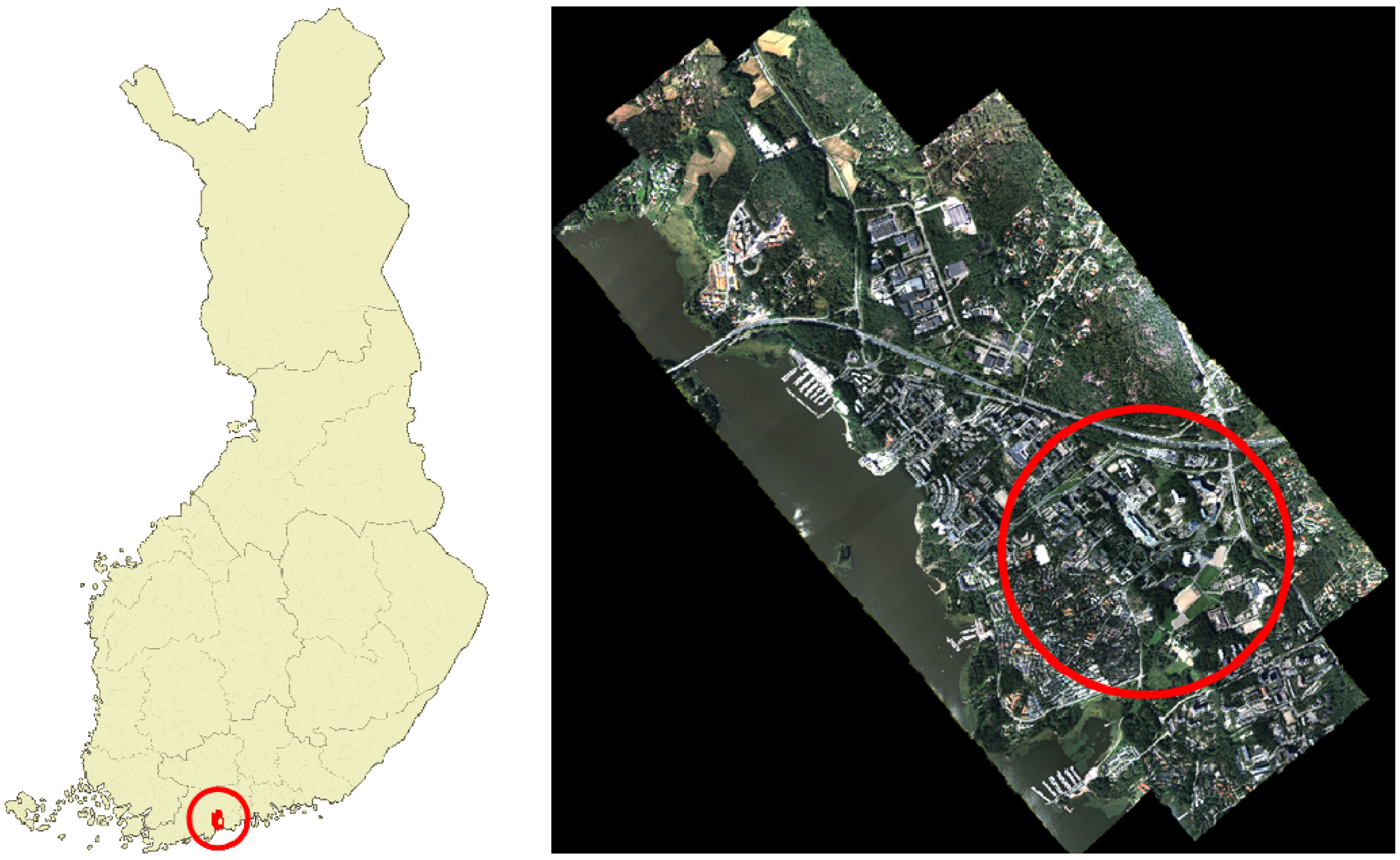
2.1. Test Area
2.2. ALS Data
2.3. Digital Aerial Images
2.4. Tree Sample Data
3. Methods
3.1. Tree Crown Delineation
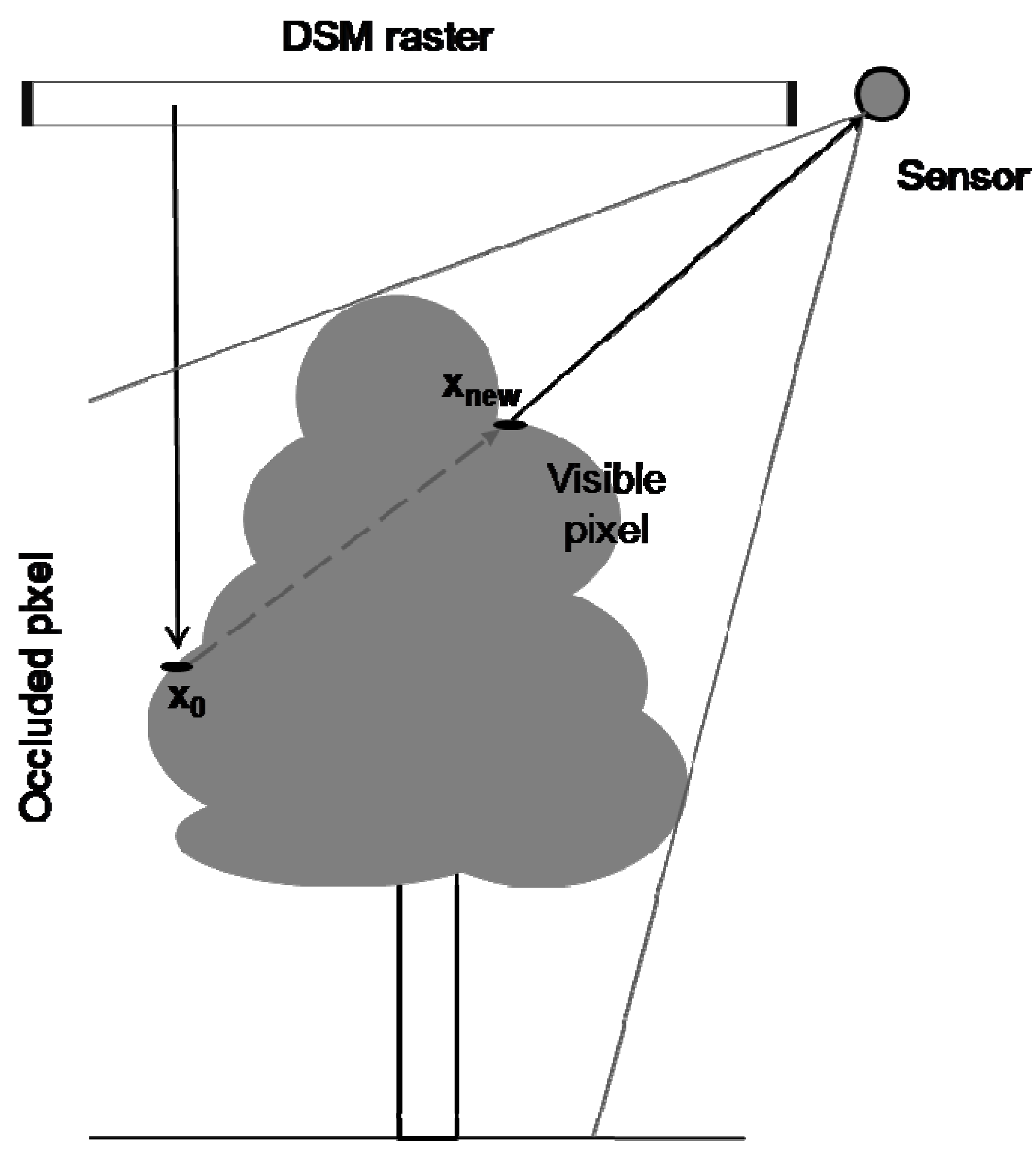
3.2. Data Cell Visibility and Shading Determination

3.3. Colour Value Extraction

3.4. Feature Set Selection
3.4.1. Illumination Dependent Colour Channels (IDCC)
3.4.2. Reference Feature Set
3.4.3. Classification Methods
4. Results
4.1. Classification Results

| Reference data | |||||||
|---|---|---|---|---|---|---|---|
| Aerial images, no filtering (linear) | Reference (Persson, [11] (linear) | ||||||
| Classification results | Birch | Pine | Spruce | Birch | Pine | Spruce | |
| Birch | 104 | 13 | 8 | 123 | 36 | 8 | |
| Pine | 34 | 73 | 14 | 17 | 45 | 15 | |
| Spruce | 13 | 13 | 23 | 11 | 18 | 22 | |
| Correctly classified | 104 | 73 | 23 | 123 | 45 | 22 | |
| Total | 151 | 99 | 45 | 151 | 99 | 45 | |
| Completeness | 68.9% | 73.7% | 51.1% | 81.5% | 45.5% | 48.9% | |
| Overall accuracy | 67.8% | 64.4% | |||||
| Coniferous vs. deciduous | 76.9% | 75.6% | |||||
| IDCC (quadratic) | Five step classifier (linear & quadratic) | ||||||
| Classification results | Birch | Pine | Spruce | Birch | Pine | Spruce | |
| Birch | 106 | 12 | 8 | 114 | 10 | 4 | |
| Pine | 32 | 78 | 12 | 25 | 77 | 12 | |
| Spruce | 13 | 9 | 25 | 12 | 12 | 29 | |
| Correctly classified | 106 | 78 | 25 | 114 | 77 | 29 | |
| Total | 151 | 99 | 45 | 151 | 99 | 45 | |
| Completeness | 70.2% | 78.8% | 55.6% | 75.5% | 77.8% | 64.4% | |
| Overall accuracy | 70.8% | 74.5% | |||||
| Coniferous vs. deciduous | 78.0% | 82.7% | |||||
4.2. Factors Affecting the Quality of Results
4.3. Further Development
5. Conclusions
Acknowledgements
References
- Næsset, E. Determination of mean tree height of forest stands using airborne laser scanner data. ISPRS J. Photogramm. Remote Sens. 1997, 52, 49–56. [Google Scholar] [CrossRef]
- Næsset, E. Predicting forest stand characteristics with airborne scanning laser using a practical twostage procedure and field data. Remote Sens. Environ. 2002, 80, 88–99. [Google Scholar] [CrossRef]
- Hyyppä, J.; Inkinen, M. Detecting and estimating attributes for single trees using laser scanner. Photogramm. J. Finl. 1999, 16, 27–42. [Google Scholar]
- Goetz, S.; Steinberg, D.; Dubayah, R.; Blair, B. Laser remote sensing of canopy habitat heterogeneity as a predictor of bird species richness in an eastern temperate forest, USA. Remote Sens. Environ. 2007, 108, 254–263. [Google Scholar] [CrossRef]
- Maltamo, M.; Packalén, P.; Peuhkurinen, J.; Suvanto, A.; Pesonen, A.; Hyyppä, J. Experiences and possibilities of ALS based forest inventory in Finland. Int. Arch. Photogramm. Remote Sens. Spatial Inf. Sci. 2007, 36, 270–279. [Google Scholar]
- Franklin, J.; Phinn, S.R.; Woodcock, C.E.; Rogan, J. Rationale and Conceptual Framework for Classification Approaches to Assess Forest Resources and Properties; Kluwer Academic Publishers: Boston, MA, USA, 2003. [Google Scholar]
- Falkowski, M.J.; Evans, J.S.; Martinuzzi, S.; Gessler, P.E.; Hudak, A.T. Characterizing forest succession with LIDAR data: an evaluation for the Inland Northwest, USA. Remote Sens. Environ. 2009, 113, 946–956. [Google Scholar] [CrossRef]
- Donoghue, D.N.M.; Watt, P.J.; Cox, N.J.; Wilson, J. Remote sensing of species mixtures in conifer plantations using LiDAR height and intensity data. Remote Sens. Environ. 2007, 110, 509–522. [Google Scholar] [CrossRef]
- Ørka, H.O.; Næsset, E.; Bollandsås, O.M. Classifying species of individual trees by intensity and structure features derived from airborne laser scanner data. Remote Sens. Environ. 2009, 113, 1163–1174. [Google Scholar] [CrossRef]
- Korpela, I.; Tuomola, T.; Tokola, T.; Dahlin, B. Appraisal of seedling stand vegetation with airborne imagery and discrete-return LiDAR an exploratory analysis. Silva Fenn. 2008, 42, 753–772. [Google Scholar] [CrossRef]
- Persson, Å.; Holmgren, J.; Söderman, U.; Olsson, H. Tree species classification of individual trees in Sweden by combining high resolution laser data with high resolution near-infrared digital images. Int. Arch. Photogramm., Remote Sens. Spatial Inf. Sci. 2004, 36, 204–207. [Google Scholar]
- Heinzel, J.N.; Weinacker, H.; Koch, B. Full automatic detection of tree species based on delineated single tree crowns a data fusion approach for airborne laser scanning data and aerial photographs. In Proceedings of Silvilaser 2008: 8th International Conference on LiDAR Appli-cations in Forest Assortment and Inventory, Edinburgh, UK, September 17–19, 2008.
- Bork, E.W.; Su, J.G. Integrating LIDAR data and multispectral imagery for enhanced classification of rangeland vegetation: a meta-analysis. Remote Sens. Environ. 2007, 111, 11–24. [Google Scholar] [CrossRef]
- Waser, L.T.; Ginzler, C.; Kuechler, M.; Baltsavias, E. Potential and limits of extraction of forest attributes by fusion of medium point density LiDAR data with ADS40 and RC30 images. In Proceedings of Silvilaser 2008: 8th International Conference on LiDAR Applications in Forest Assortment and Inventory, Edinburgh, UK, September 17–19, 2008.
- Kim, S.; McGaughey, R.J.; Andersen, H.E.; Schreuder, G. Tree species differentiation using intensity data derived from leaf-on and leaf-off airborne laser scanner data. Remote Sens. Environ. 2009, 113, 1575–1586. [Google Scholar] [CrossRef]
- Meyer, P.; Staenz, K.; Itten, K.I. Semi-automated procedures for tree species identification in high spatial resolution data from digitized colour infrared aerial photography. ISPRS J. Photogramm. Remote Sens. 1996, 51, 5–16. [Google Scholar] [CrossRef]
- Kaartinen, H.; Hyyppä, J. Tree Extraction. In EuroSDR Official Publication; Report of EuroSDR project, 53; EuroSDR: Frankfurt, A.M., Germany, 2008; p. 60. [Google Scholar]
- Kaasalainen, S.; Rautiainen, M. Backscattering measurements from individual Scots pine needles. Appl. Opt. 2007, 46, 4916–4922. [Google Scholar] [CrossRef] [PubMed]
- Chen, J.M.; Leblanc, S.G. Multiple-scattering scheme useful for geometric optical modeling. IEEE Trans. Geosci. Remote Sens. 2001, 39, 1061–1071. [Google Scholar] [CrossRef]
- Hall, F.G.; Hilker, T.; Coops, N.; Lyapustin, A.; Huemmrich, K.F.; Middleton, E.; Margolis, H.; Drolet, G.; Black, T.A. Multi-angle remote sensing of forest light use efficiently by observing PRI variation with canopy shadow fraction. Remote Sens. Environ. 2008, 112, 3201–3211. [Google Scholar] [CrossRef]
- Hilker, T.; Coops, N.; Hall, F.G.; Black, T.A.; Wulder, M.A.; Krishnan, Z.N.P. Separating physiologically and directionally induced changes in PRI using BRDF models. Remote Sens. Environ. 2008, 112, 2777–2788. [Google Scholar] [CrossRef]
- Korpela, I. Individual Tree Measurements by Means of Digital Aerial Photogrammetry. Ph.D. Thesis, University of Helsinki, Helsinki, Finland, 2004. [Google Scholar]
- Larsen, M. Single tree species classification with a hypothetical multi-spectral satellite. Remote Sens. Environ. 2007, 110, 523–532. [Google Scholar] [CrossRef]
- Dralle, K.; Rudemo, M. Stem number estimation by kernel smoothing of aerial photos. Can. J. For. Res. 1996, 1228–1236. [Google Scholar] [CrossRef]
- Gougeon, F.A. A crown-following approach to the automatic delineation of individual tree crowns in high spatial resolution aerial images. Can. J. Remote Sens. 1995, 274–284. [Google Scholar] [CrossRef]
- Larsen, M.; Rudemo, M. Optimizing templates for finding trees in aerial photographs. Pattern Recognit. Lett. 1998, 19, 1153–1162. [Google Scholar] [CrossRef]
- Bang, K.; Habib, A.; Shin, S.; Kim, K. Comparative analysis of alternative methodologies for true ortho-photo generation from high resolution satellite imagery. In Am. Soc. Photogramm. Remote Sens. (ASPRS) Annual Conference: Identifying Geo-Spatial Solution, Tampa, FL, USA, May 7–11, 2007.
- Roy, V. Sun position calculator for MATLAB. 2004. Available online: http://www.mathworks.com/matlabcentral/fileexchange/4605 (accessed on August 5, 2008).
- Reda, I.; Andreas, A. Solar Position Algorithm for Solar Radiation Application; Technical Report NREL/TP-560-34302; NREL Golden, Co, USA, 2003. Available online: http://www.nrel.gov/docs/fy08osti/34302.pdf (accessed on August 5, 2008).
- Kraus, K. Photogrammetry: Fundamentals and Standard Processes, 4th ed.; Kraus, K., Ed.; Dümmler: Bonn, Germany, 1993. [Google Scholar]
- Rautiainen, M.; Nilson, T.; Lükk, T. Seasonal reflectance trends of hemiboreal birch forests. Remote Sens. Environ. 2009, 113, 805–815. [Google Scholar] [CrossRef]
- Litkey, P.; Rönnholm, P.; Lumme, J.; Liang, X. Waveform features for tree identification. Int. Arch. Photogramm. Remote Sens. Spatial Inf. Sci. 2007, 36, 258–263. [Google Scholar]
- Hyyppä, J.; Hyyppä, H.; Litkey, P.; Yu, X.; Haggrèn, H.; Rönnholm, P.; Pyysalo, U.; Pitkänen, J.; Maltamo, M. Algoritms and methods of airborn laser scanner for forest measurements. Int. Arch. Photogramm. Remote Sens. Spatial Inf. Sci. 2004, 36, 82–89. [Google Scholar]
- Koch, B.; Heyder, U.; Weinacker, H. Detection of individual tree crowns in airborne LIDAR data. Photogramm. Eng. Remote Sens. 2006, 72, 357–363. [Google Scholar] [CrossRef]
- Pouliot, D.A.; King, D.J.; Pitt, D.G. Development and evaluation of an automated tree detection-delineation algorithm for monitoring regenerating coniferous forests. Can. J. For. Res. 2005, 35, 2332–2345. [Google Scholar] [CrossRef]
- Erikson, M.; Olofsson, K. Comparison of three individual tree crown detection methods. Mach. Vis. Appl. 2005, 16, 258–265. [Google Scholar] [CrossRef]
© 2010 by the authors; licensee Molecular Diversity Preservation International, Basel, Switzerland. This article is an open-access article distributed under the terms and conditions of the Creative Commons Attribution license (http://creativecommons.org/licenses/by/3.0/).
Share and Cite
Puttonen, E.; Litkey, P.; Hyyppä, J. Individual Tree Species Classification by Illuminated—Shaded Area Separation. Remote Sens. 2010, 2, 19-35. https://doi.org/10.3390/rs2010019
Puttonen E, Litkey P, Hyyppä J. Individual Tree Species Classification by Illuminated—Shaded Area Separation. Remote Sensing. 2010; 2(1):19-35. https://doi.org/10.3390/rs2010019
Chicago/Turabian StylePuttonen, Eetu, Paula Litkey, and Juha Hyyppä. 2010. "Individual Tree Species Classification by Illuminated—Shaded Area Separation" Remote Sensing 2, no. 1: 19-35. https://doi.org/10.3390/rs2010019