Dynamic Spatial–Spectral Feature Optimization-Based Point Cloud Classification

Abstract

With the development and popularization of LiDAR technology, point clouds are becoming widely used in multiple fields. Point cloud classification plays an important role in segmentation, geometric analysis, and vegetation description. However, existing point cloud classification algorithms have problems such as high computational complexity, a lack of feature optimization, and low classification accuracy. This paper proposes an efficient point cloud classification algorithm based on dynamic spatial–spectral feature optimization. It can eliminate redundant features, optimize features, reduce computational costs, and improve classification accuracy. It achieves feature optimization through three key steps. First, the proposed method extracts spatial, geometric, spectral, and other features from point cloud data. Then, the Gini index and Fisher score are used to calculate the importance and relevance of features, and redundant features are filtered. Finally, feature importance factors are used to dynamically enhance the discriminative power of highly distinguishable features to strengthen their contribution to point cloud classification. Four real-scene datasets from STPLS3D are utilized for experimentation. Compared to the other five algorithms, the proposed algorithm achieves at least a 37.97% improvement in mean intersection over union (mIoU). Meanwhile, the results indicate that the proposed algorithm can achieve high-precision point cloud classification with low computational complexity.

1. Introduction

LiDAR has been widely used in many fields, such as urban planning [1], autonomous driving [2], agricultural development [3], and land use change [4]. Unlike 2D detection based on image data from optical sensors, LiDAR’s spatial sensing capabilities are advantageous for object recognition in 3D spaces [5]. LiDAR is a radar system that detects a target’s position, velocity, and other characteristic parameters by emitting a laser beam [6]. Compared to traditional two-dimensional remote sensing data, the point cloud contains geometric information and potentially encompasses information about color or intensity [7]. Due to these advantages, more researchers have begun exploring the area of 3D space. Three-dimensional point cloud semantic segmentation and recognition algorithms hold significance in computer vision as a long-standing research topic [8]. However, the disorder and irregularity of point clouds in 3D space pose challenges for the automatic and accurate classification of point clouds [9,10].

In early research on the topic, some scholars employed the technique of rasterizing 3D point clouds. The underlying principle involves projecting the 3D point cloud onto a 2D plane and subsequently leveraging existing 2D image processing methods to extract features for further processing [11]. RangeNet++, proposed by Milioto et al., is one of these representative methods [12], which is inspired by the TangentConv network [13] and SqueezeSeg V2 network [14] methods. RangeNet++ preserves the projection of point cloud data onto a sphere, resulting in a 2D image representation akin to a distant image. Classification is performed on the 2D image, and the results are subsequently mapped back to the 3D space. However, this projection process inevitably leads to losing geometric relationships and structural information in the 3D point cloud space [7].

Drawing inspiration from the processing of 2D images, Maturana et al. were the first to propose voxelized point clouds by dividing them into evenly spaced voxel grids and feeding them into a convolutional neural network [15]. Since then, OctNet [16], MV3D [17], and other networks and algorithms have been proposed. While voxel-based point cloud classification techniques, to some extent, preserve the 3D geometric relationships and structures of point clouds, the choice of voxel size during the voxelization process can influence the classification results. Using overly large voxels can lead to the loss of geometric details, while using overly small voxels can increase computational costs [7].

Methods that transform point cloud data into regular and structured 3D voxel grids or collections of images can result in unnecessarily large data. Therefore, researchers have proposed deep learning-based approaches that handle point cloud data directly. Qi Charles first proposed PiontNet, which is pioneering in the direct classification of original point clouds [18]. Based on PointNet and PointNet++ [19], RandLA-Net [9] introduces an efficient local feature aggregation module that progressively increases the receptive field of each point, allowing for better learning and the preservation of complex geometric structures within large-scale point clouds. The experiments demonstrate that RandLA-Net achieves high efficiency in terms of memory and computation while achieving significant overall performance. Although those deep learning-based methods mentioned above have achieved good performances in extracting local features, some of these methods have a high computational complexity. This prevents the design of deeper network structures, leading to insufficient semantic information extraction and compromised accuracy, especially in large-scale point cloud scenes [20].

Some researchers have attempted to combine traditional features with machine learning (ML) and deep learning (DL) for point cloud classification. Zhao et al. combined existing DL network models with four shallow features: normalized height, surface roughness, intensity, and the normalized vegetation index, to classify the ISPRS dataset. The classification accuracy reached 87.1% [21]. Poliyapram et al. proposed the PMNet network, which utilizes the combination of intensity and RGB features to classify ALS point clouds of Osaka City. The experiments demonstrated that the overall accuracy was improved from 65% to 79% [22]. Li et al. employed geometric matrix enhancement to describe the geometric features of point clouds [23]. Additionally, they utilized spectral information from multispectral point cloud data to further enhance classification accuracy. Xiu et al. associated point cloud data with color features from orthoimages in a point cloud classification. By incorporating color features, the overall accuracy improved by 2% [24]. These methods are prone to overfitting, and due to their large model sizes, they require significant computational resources. Harith Aljumaily et al. [25] utilized five point descriptors (density, standard deviation, clustered points, fitted plane, and plane’s angle) and two voxel location attributes (elevation and neighbors) to describe the distribution of points within voxels and the geographical location of voxels. Finally, they employed a random forest (RF) classifier for data analysis. The experimental results indicate excellent average precision performance. RF is a computationally efficient ML method that can achieve a higher accuracy than other methods without requiring extensive training time [25]. Furthermore, due to its strong robustness and resistance to overfitting [26], since its first application in point cloud data classification, it has been consistently used in this field and still holds great potential [27].

In summary, existing methods that combine traditional feature extraction with machine learning are known for their real-time performance and their ability to achieve a high classification accuracy. However, these methods often lack feature optimization and selection and face the risk of dimension explosion and performance degradation as the number of features to be processed increases. At the same time, these methods require substantial computational resources and time investments. Therefore, this paper designs multiple spectral-spatial feature extraction algorithms and uses the RF algorithm, with its strong anti-overfitting and excellent deep-shallow feature extraction ability, as the classifier to propose a large-scale point cloud classification method based on dynamic spatial–spectral feature optimization. Through experiments, it has been proven that this method can achieve robustness and a high classification accuracy. The main contributions of this paper are as follows:

(1) This paper adopts a multi-domain feature extraction method based on statistical analysis and machine learning to obtain spatial, geometric, spectral, and other deep features from point cloud data. It also proposes using the Gini Index and Fisher Score to calculate feature importance and correlation. Finally, comprehensively assessing importance and relevance promotes effectively filtering shallow and deep features, thereby eliminating feature redundancy.

(2) This paper proposes a point cloud classification method based on spatial–spectral feature-weighted fusion and RF. After feature filtering, it dynamically enhances the discriminative power of features with a high separability using feature importance factors, effectively combines multiple shallow and deep features, and improves their contribution to point cloud classification, thereby ensuring high-precision point cloud classification.

2. Materials and Methods

2.1. Datasets

Semantic Terrain Points Labeling–Synthetic 3D dataset (STPLS3D) [28] has four real-world sites, including the University of Southern California Park Campus (USC), Wrigley Marine Science Center (WMSC) located on Catalina Island, Orange County Convention Center (OCCC), and a residential area (RA). These four regions are shown in Figure 1. This dataset was collected using a crosshatch-type flight pattern with flight altitudes ranging from 25–70 m in 2021.

All four regions have distinct features, with significant differences in land cover categories and quantities. Each data sample category and quantity are displayed in the

Table 1. The proportion information in each category in the STPL3D dataset.

	RA	WMSC	OCCC	USC
Building	2,388,323 (34.99%)	996,180 (9.98%)	14,742,339 (37.88%)	40,094,389 (42.34%)
Low vegetation	1,460,336 (21.10%)	2,086,770 (20.91%)	6,685,428 (17.18%)	27,996,830 (29.57%)
Vehicle	133,085 (1.95%)	42,033 (0.42%)	964,766 (2.48%)	478,130 (0.50%)
Light Pole	18,870 (0.28%)	6,232 (0.06%)	74,233 (0.19%)	179,555 (0.19%)
Clutter	32,383 (0.47%)	134,859 (1.35%)	145,289 (0.37%)	2,112,812 (2.23%)
Fence	333,862 (4.89%)	76,296 (0.76%)	56,405 (0.14%)	819,305 (0.87%)
Road	2,054,448 (30.10%)	754,171 (7.56%)	8,636,482 (22.19%)	16,051,158 (16.95%)
Dirt	32,315 (0.47%)	4,700,616 (47.11%)	1,393,234 (3.58%)	828,581 (0.88%)
Grass	371,443 (5.44%)	1,180,607 (11.83%)	6,216,458 (15.97%)	6,134,089 (6.48%)
Total	6,825,065 (100%)	9,977,764 (100%)	38,914,634 (100%)	94,694,849 (100%)

and Figure 2.

RA: The RA region is a typical residential area. The buildings are neatly arranged, and their height does not exceed three floors.

WMSC: The WMSC region is an area which is different to the urban environment. There are fewer buildings, and a larger portion is covered by bare land and grassland.

OCCC: The OCCC region includes a large convention center and its surrounding environment. Fewer tall buildings, mostly scattered vegetation, and concentrated parking lots exist.

USC: The USC area is mainly covered by tall buildings, accounting for approximately 42% of land cover. The grassland coverage rate is about 6.5%. The proportions of categories such as vehicles, light poles, fences, and dirt are all less than 1%.

From Figure 2, it can be seen that there is a significant difference in the label counts between different categories within the same dataset. The “Light Pole” category is consistently the least represented across different datasets. Comparing the data in Table 1, it can be observed that there are significant differences in the proportions of the same category across different datasets. The phenomenon of the same category also has similar proportions across different datasets. These phenomena indicate that the experimental data have the capability of cross-validation. The experimental data can be used as training and testing samples for each other.

2.2. The Proposed Method

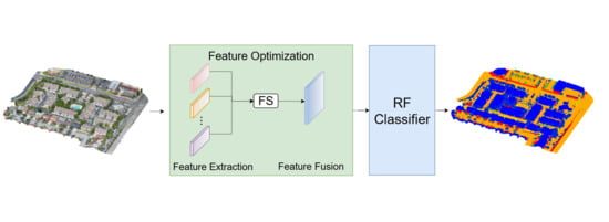
The proposed point cloud classification method comprises five main steps: ① Voxel downsampling is applied to the experimental data. ② Feature extraction is performed on the data. ③ Feature importance and correlation are calculated for the extracted features, and low-importance features are removed. ④ Feature fusion is conducted based on step three’s results, considering feature importance. ⑤ The feature set obtained after weighted fusion is fed into an RF classifier to generate classification results. To clearly illustrate the algorithm flow, the overall description of the proposed method is shown in Algorithm 1. The details of the main steps will be described in the following sections.

2.2.1. Voxel Preprocessing

The principle of voxel grid filtering involves partitioning the point cloud data into a grid of cubic voxels, computing representative points for each grid, and replacing all the points within a voxel with its representative point. This process achieves downsampling. Due to the different choice of representative points, two voxel downsampling methods, voxel grid (Equation (1)) and approximate voxel grid (Equation (2)), have been generated. The former employs the center point of each voxel as the representative point, while the latter uses the centroid of each voxel as the representative point. This paper illustrates the difference between the two downsampling methods through specific examples. The voxel size for both methods was set to 0.5 × 0.5 × 0.5. The experimental results are shown in Figure 3. The original point cloud consisted of 7501 points, and after downsampling, the point counts were reduced to 674 and 1156, respectively. With the same voxel block size, the two methods will filter out different numbers of points, resulting in different results. The three images in Figure 3 show that, although the Voxel Grid method results in roughly complete object contours, some fine-grained local shape details in the original point cloud are lost. The results of approximate voxel grid method still retain the detailed information from the original point cloud, which will be beneficial for improving the subsequent classification accuracy. Therefore, this paper chooses the approximate voxel grid method.

$$\left\{\begin{array}{c}x=\frac{{\sum }_i^m{x}_i}{m}\hfill \\ y=\frac{{\sum }_i^m{y}_i}{m}\hfill \\ z=\frac{{\sum }_i^m{z}_i}{m}\hfill \end{array}\right.$$

(1)

where $(x,y,z)$ represent the centroid within a voxel containing m points. $(x_i,y_i,z_i)$ represent points within the voxel.

$$\left\{\begin{array}{c}{x}_{center}=x_{min}+(c_i-0.5)\ast 0.5\hfill \\ y_{center}=y_{min}+(r_i-0.5)\ast 0.5\hfill \\ z_{center}=z_{min}+(l_i-0.5)\ast 0.5\hfill \end{array}\right.$$

(2)

where $(x_{center},y_{center},z_{center})$ are the center of the voxel being solved. $(c_i,r_i,l_i)$ represent the number of rows and columns in which $(x_i,y_i,z_i)$ are located. $(x_{min},y_{min},z_{min})$ represent the minimum coordinate value in the voxel.

Algorithm 1 Large-scale point cloud classification using random forest based on weighted feature spatial transformation

Input: $D={\left\{x_n,y_n,z_n\right\}}_{n=1}^N$: Point cloud dataset 1: Preprocess D using voxel filter to obtain $D_1={\left\{x_i,y_i,z_i\right\}}_{i=1}^M$ 1. 2: Extract features from $D_1$ to obtain the feature set $\mathbf{F}={\left[F_{1g},F_{2g},F_{3g},\cdots ,F_{kg}\right]}^T$2. The features include the following: ① Comparative features of spectral information: $F_{1g}=I\left(P_g,c_g\right)-I\left(P_{g+1},c_{g+1}\right)$; ② Spatial information distribution feature: $F_{2g}$; ③ Global feature: $F_{3g}$; ④ Localized spatial enhancement features: $F_{4g}$; ⑤ Elevation feature: $F_{5g}$; ⑥ Plane roughness: $F_{6g}=\left|A{x}_o+B{y}_o+C{z}_o+D\right|/\phantom{\left|A{x}_o+B{y}_o+C{z}_o+D\right|\sqrt{A^2+B^2+C^2}}\sqrt{A^2+B^2+C^2}$. 3: Calculate feature importance using the Gini Index (Equation (11)) to obtain feature importance factors $W={\left\{w_k\right\}}_{k=1}^6$. Calculate feature correlation using the Fisher Score (Equation (12)). 4: Select the optimal feature set. Comprehensively evaluate the importance and relevance of features and conduct feature selection to obtain feature set ${\mathbf{F}}_s={\left[F_{1g},F_{2g},\cdots ,F_{sg}\right]}^T$. 5: Fuse feature set ${\mathbf{F}}_s$ to obtain $F_f$. Combine the optimal feature set ${\mathbf{F}}_s$ with feature importance factors using Equation (13) to obtain $F_f$. 6: Input $F_f$ into the RF classifier. Output: The classification results. 1 M represents the number of point clouds in data. 2 $F_{k}g$ represents the feature of a point.

2.2.2. Feature Extraction Based on Statistical Analysis and Spatial–Spectral Information

Point cloud data attributes typically include three coordinates (x,y,z) and intensity data or color information [25]. Point cloud data contain more comprehensive and detailed information about the target objects. This paper extracts the comparative features of spectral information, spatial information distribution features, global features, localized spatial enhancement features, elevation features, and plane roughness to better describe the target objects within the point cloud dataset.

• Comparative features of spectral information

Comparative features of spectral information are a type of feature used to calculate the similarity or dissimilarity between different points [29,30]. It typically involves comparing the attributes of two points, such as color, depth, etc., to determine the similarity or dissimilarity between the two points. We randomly select two adjacent points for each point and calculate the difference between them using Equation (3).

$$F_{1g}=I\left(p+\frac{{\delta }_1}{D\left(p\right)},c_1\right)-I\left(p+\frac{{\delta }_2}{D\left(p\right)},c_2\right)$$

(3)

where p is the m-th pixel, $\delta$ represents the window offset, $D\left(p\right)$ represents the depth pixel, and $I\left(p,c\right)$ denotes the RGB pixel lookup in channel c.

Since this feature is represented by comparing the RGB and depth information from adjacent points, it contains detailed contextual information, making it easy to capture the details of the target in complex scenes [31].

• Spatial information distribution features

The spatial information distribution features mainly describe the distribution of points. This paper employs the Density-Based Spatial Clustering of Applications with Noise (DBSCAN) [32] clustering algorithm. The DBSCAN algorithm is a density-based clustering method used to identify dense regions in data and group them into clusters. The basic diagram of the definition of DBSCAN is shown in Figure 4. It is based on a set of “neighborhood” parameters $\left(\in ,MinPts\right)$ to characterize the tightness of the sample distribution. Unlike traditional distance-based clustering algorithms like K-means, DBSCAN determines the shape and size of clusters based on the density relationships between data points. This paper generates features represented as $F_{2g}$ by counting the number of points in each cluster. And then associates each point in the point cloud data with each cluster.

$$F_{2g}=\left\{b_1,b_2,b_g,\cdots b_M\right\}$$

(4)

where $b_m$ represents the number of points associated with the m-th point in the cluster.

The advantage of DBSCAN lies in its ability to discover clusters of arbitrary shapes and its robustness against noisy data [33]. It can automatically determine the number of clusters and is not constrained by the shape or size of clusters [34].

• Global features

Global features are used to describe the characteristics of the entire dataset or object. It focuses on describing not only individual data points or object attributes but also the data’s overall distribution, relationships, or attributes. For point cloud data $D_1$ composed of M points, first use Equation (5) to determine its symmetric positive definite covariance matrix. Calculate the eigenvalues and eigenvectors of matrix $\mathbf{T}$. The eigenvalues are represented by ${\overrightarrow{e}}_1$,${\overrightarrow{e}}_2$ and ${\overrightarrow{e}}_3$, respectively, and the eigenvectors are represented by ${\lambda }_1$, ${\lambda }_2$ and ${\lambda }_3$, with ${\lambda }_1\ge {\lambda }_2\ge {\lambda }_3$. Then, ${\lambda }_1$, $\left({\lambda }_1-{\lambda }_2\right){\overrightarrow{e}}_1$, and $\left({\lambda }_2-{\lambda }_3\right){\overrightarrow{e}}_3$ define the three-dimensional local structure points, curvature, and surface degree. Finally, the three-dimensional local structural features of each point and its neighborhood are counted by using histograms. And data calculations can be carried out on the results to convert the 3D local features into global features ($F_{3g}$).

$$\mathbf{T}=\frac{1}{M}\sum _{i=1}^M\left(X_i-\overline{X}\right){\left(X_i-\overline{X}\right)}^T$$

(5)

where $\left\{X_j\right\}=\left\{{\left(x_j,y_j,z_j\right)}^T\right\}$ and $\overline{X}=\left(1/\phantom{1M}M\right){\sum }_{j=1}^M{X}_i$.

$$F_{3g}=\left\{f_{3g},f_{3g},\cdots ,f_{3g},\cdots ,f_{3G}\right\}$$

(6)

• Localized spatial enhancement features

Localized spatial enhancement features enhance feature representations by incorporating contextual information within a local spatial region. First, the k-Nearest Neighbor algorithm (KNN) [35] is used to collect the neighboring points of the g-th point. Then, Equation (7) encodes point g and its neighboring points based on Euclidean distance. Afterward, through Equation (8), $v_g$ is associated with its corresponding point feature $f_g$ to obtain enhanced feature $F_{4g}^k$.

$$u_g=MLP\left(v_g\oplus v_g^k\oplus \left(v_g-v_g^k\right)\oplus ∥v_g-v_g^k∥\right)$$

(7)

where ⊕ is series operation. $v_g$ and $v_g^k$ represent the x–y–z coordinates of point g and its K-nearest neighbor points. $∥·∥$ is used to calculate the Euclidean distance between the adjacent point and the center point [9,18].

$$F_{4g}=\left\{u_1:f_1,u_2:f_2,\cdots ,u_g:f_g,\cdots ,u_M:f_M\right\}$$

(8)

where $f_g$ represents the geometric feature corresponding to point g.: represents the association operator.

• Elevation features and plane roughness

This paper uses the standard deviation (Equation (9)) to describe the elevation features in the point cloud. It is commonly used to characterize the variability or dispersion among points in point cloud data.

$$F_{5g}=\sqrt{\sum _{g=1}^M{\left(z_g-\overline{z}\right)}^2}/\phantom{\sqrt{\sum _{g=1}^M{\left(z_g-\overline{z}\right)}^2}\sqrt{M}}\sqrt{M}$$

(9)

where $z_g$ represents the elevation of the g-th point, and $\overline{z}$ represents the mean elevation.

Plane roughness refers to a feature that describes the irregularity of a planar surface within a point cloud. Typically, it is quantified by calculating the distance from a selected point to the plane that best fits that point, as expressed in Equation (10).

$$F_{6g}=\left|A{x}_o+B{y}_o+C{z}_o+D\right|/\phantom{\left|A{x}_o+B{y}_o+C{z}_o+D\right|\sqrt{A^2+B^2+C^2}}\sqrt{A^2+B^2+C^2}$$

(10)

where $A{x}_o+B{y}_o+C{z}_o+D=0$ represents the fitted plane obtained based on the least squares principle.

2.2.3. Feature Selection and Feature Fusion

This section provides a detailed explanation of feature selection based on feature importance and correlation. Firstly, feature importance and correlation are calculated using the Gini Index and Fisher Score. Subsequently, comprehensively assessing importance and relevance promotes effective filtering of shallow and deep features, thereby eliminating feature redundancy. After completing feature selection, feature fusion is implemented. This dynamically enhances the discriminative power of features with high separability using feature importance factors.

• Feature selection based on feature importance and correlation

Learning methods often tend to overfit in situations with many irrelevant and/or redundant features, leading to reduced interpretability [36,37,38]. Therefore, this paper proposes a feature selection based on importance and correlation to improve the efficiency and performance of the algorithm.

Feature importance is a measure used to assess each feature’s relative importance in or contribution to predicting the target variable. In this paper, the Gini Index is chosen to calculate the importance of features. Supposing that n features are extracted, the importance of feature $F_m^k$ is calculated by Equation (11).

$$G{I}_m^K=1-\sum _{k=1}^K\left(f_m^k\right)$$

(11)

where K represents the number of features, and $F_m^k$ represents the proportion of the k-th feature in node m.

As shown in Figure 5, for the experimental data, the first four features are relatively important: comparative features of spectral information, spatial information distribution features, global features, and localized spatial enhancement features.

Feature correlation refers to the degree of association between different features within a dataset. It is used to measure whether there is a relationship between features and to assess the strength and direction of this relationship. Fisher score is one of the most widely used supervised feature selection methods [36]. In this paper, the fisher scores [39] are selected to calculate the relevance of features. The equation is as follows:

$$S_k=\frac{{\displaystyle \sum _{j=1}^C}\frac{n_j}{n}{\left({\overline{F}}_{jm}^k-{\overline{F}}^k\right)}^2}{\frac{1}{n}{\displaystyle \sum _{j=1}^C}{\displaystyle \sum _{x\in w_j}}{\left(x^k-{\overline{F}}_{jm}^k\right)}^2}$$

(12)

where C is the total number of categories, $n_j$ is the number of j-th category points, n is the total number of samples, ${\overline{F}}_{jm}^k$ is the mean value of the m-th point on the k-th feature, ${\overline{F}}^k$ is the mean value of all category points on the k-th feature, $x^k$ is the value of point m on the k-th feature, and $w_j$ is the j-th category.

• Multi-features weighted fusion

Feature fusion refers to the process of combining data from different information sources or feature extraction methods to enhance the performance and expressive capabilities of a model [40]. Feature fusion is commonly employed to combine features of different types, origins, or representations to help the model better understand data for prediction or classification [41]. So far, numerous feature fusion methods have been proposed. Among them, using operations like summation or concatenation to achieve feature fusion is a simple method [42]. For different network scenarios, this might not always be the optimal choice [43].

To ensure that more informative features contribute significantly to the fused result, this paper employs a weighted fusion approach based on feature importance and correlation. After feature selection, feature fusion is performed by combining the features with feature importance factors using the following formula:

$$F_f=\sum _{k=1}^K{w}_k{F}_{km}$$

(13)

where $w_k$ is the feature importance factor of the k-th feature, which is numerically equal to $I_{Fq}^k$.

2.2.4. Classification with RF

First, the features extracted in this paper are subjected to feature selection and feature fusion. Then, the obtained effective feature tensors $F_f$ are input into the RF classifier for point cloud classification. RF is an ensemble learning method based on decision trees [44,45]. It enhances prediction accuracy and stability by constructing multiple decision trees. Each decision tree consists of split points and leaf nodes. Nodes represent features, and leaf nodes represent a class or a value. That is, each decision tree is constructed from random samples and random features. Therefore, RF can avoid over-fitting phenomena (Figure 6 shows a schematic diagram of the working principle of the RF classifier). Compared to the Support Vector Machine (SVM) and K-means algorithm, RF has features such as high accuracy and strong robustness [46]. Among them, the ability to handle a large number of input features randomly is the main reason for choosing this classifier.

2.2.5. Evaluation Index

In this paper, mean intersection over union (mIoU), overall accuracy (OA), average accuracy (AA), F-Measure, minRecall, G-mean, and confusion matrix are utilized for quantitative evaluation of the classification results. Here is a brief introduction to IoU, OA, and the confusion matrix. IoU, which evaluates the performance of the approach, calculates the intersection between predicted value and ground truth divided by the union of both. mIoU averages all IoU values by each class, which is defined in Equation (14). OA, which evaluates the classification accuracy of a classification method, is the ratio between the number of samples classified in a specific class and the total number of samples (Equation (15)). The confusion matrix summarizes the records in the dataset in the form of a matrix according to two criteria: the real category and the category judgment predicted by the classification model.

$$mIoU=\frac{1}{L}\sum _{i=1}^L\frac{P\cap G}{P\cup G}$$

(14)

where P is the prediction number of the i-th class. G is the ground truth number of the i-th class.

$$OA=\sum _{i=1}^L\frac{con{f}_{ii}}{{\sum }_j^{L}con{f}_{ij}}$$

(15)

where $con{f}_{ij}$ represents the value of the i row and j column in the confusion matrix.

3. Results

3.1. Classification Accuracy

Figure 7 shows the classification accuracy of each category in the four datasets after applying the proposed algorithm. Figure 8 shows the mIoU of each category in the four datasets after applying the proposed algorithm. The blue line in the figure represents the classification accuracy and mIoU of each category in the RA data. Referring to Table 1, it can be observed that the clutter and dirt categories have a proportion of around 0.47%. However, the accuracy of clutter is only about 40%, while the accuracy of sirt is approximately 90%. Even for the light pole category, which accounts for only 0.28% of the data, the accuracy exceeds 65%, significantly surpassing that of the clutter category.

The figure’s red line represents each category’s classification accuracy and mIoU in WMSC data. The proportion of the light pole category is approximately 0.06% (Table 1), the lowest among all categories. However, its classification accuracy reached 83%. This indicates that the extracted features can vividly describe the category of light poles.

By observing the yellow and green lines in the graph, it can be observed that the same situation occurs in both the OCCC and USC data. Compared to the RA and WMSC data, OCCC and USC have a considerable amount of data, and the proportion of each category varies greatly. However, for categories with a data volume ratio of less than 1%, some accuracies are still above 60%, and some even exceed 80%. This indicates that the proposed algorithm is beneficial to some extent in improving the problem of imbalanced data categories. Among these two datasets, the classification accuracy of the light pole category is the lowest.

Figure 9 shows the evaluation results of OA, AA, mIoU, Fmeasure, and other indicators for the classification results for the four datasets. Comparing the results of the RA, WMSC, and OCCC datasets, the OCCC dataset consistently has a higher accuracy regarding OA and AA. The mIoU indicator for the USC data results is below 80%. The mIoU indicators for the other three datasets are all above 80%, and the mIoU of the WMSC data is even close to 90%. The F-measure indicators for the four datasets all performed well; all were higher than 80%. Among them, the F-measure value for the OCCC data exceeded 90%. The G-mean index values of the four datasets vary significantly. The G-mean value for OCCC data exceeds 85%, while the G-mean value for the RA dataset is less than 50%.

Figure 10 shows a confusion matrix for the four data classification results. The road category’s prediction accuracy in the RA data’s confusion matrix is the highest, reaching 97.69%. The accuracy of the building category is 97.44%, with suboptimal performance. The accuracy of the clutter category is the lowest, below 50%. Observing the confusion matrix for the RA data in Figure 10a, it can be observed that there are different numbers of clutter categories mistakenly classified into other categories. Among them, there is a high possibility of being incorrectly identified as a fence, light pole, or low vegetation. We think that the reason for this occurrence can be attributed to the attributes of the clutter category. The clutter category contains many small-proportion objects, which are challenging to describe vividly, thus hindering accurate classification.

3.2. Classification Results

In the confusion matrix for the WMSC data, the building category performs the best with an accuracy of 98.32%. The road category performs suboptimally, with an accuracy of 94.96%. The fence category has the lowest accuracy. However, compared to the clutter category in the RA data, the fence category’s accuracy reaches 70.91%. In the confusion matrix for the OCCC data, the accuracy of the building category is the highest, reaching 99.75%. The dirt category has the lowest accuracy at 74.95%. In the confusion matrix for the USC data, the building category still has the highest accuracy. The light pole category has the lowest accuracy at 53.07%. Across the four datasets, the proportion of the building category varies significantly (Refer to Table 1), yet the accuracy remains consistently high with slight variation. This is due to the highly consistent density features of the building class.

Figure 11 shows a visualization of the classification results of the proposed method and the ground truth in Cloud Compare. A comparative analysis of the ground truth and classification results for the four datasets shows that the majority of land cover types can be accurately classified. All categories can be accurately classified without apparent errors.

Comparing the ground truth (Figure 11c) and classification results (Figure 11d) for the RA data, it can be found that the light pole category in the red box can be accurately classified. The tree category and vehicle categories in the figure are also clearly classified. Comparing the ground truth (Figure 11g) and classification results (Figure 11h) for the USC data, the light pole, grass, and low vegetation categories in the white box can be accurately classified. Comparing the ground truth (Figure 11f) and classification results (Figure 11e) for the OCCC data, it can be seen that the low vegetation in the white box can be accurately classified. Moreover, the category details obtained from the classification results are consistent with those in the ground truth. However, the light pole category portion in the black box was mistakenly identified as another category.

Figure 12 shows a visualization of the ground truth and classification results for the RA data light pole, low vegetation, and building categories in Cloud Compare. Figure 12b shows the light pole categories in the classification results separately. It can be seen that all light poles in the RA data have been clearly marked. Compared to Figure 12c, although there are scattered points in Figure 12d, the detailed description of the low vegetation in Figure 12d is complete. Figure 12e shows the building category’s ground truth and classification results separately. It can be seen that there are other categories marked as building categories. However, the building categories have all been classified.

3.3. Comparison with Other Methods

Five representative approaches were selected as comparison algorithms, including PointTransformer [47], RandLA-Net [9], SCF-Net [48], MinkowskiNet [49], and KPConv [50].

To be consistent with the official data categories, we have classified nine features into six categories. The ground category includes grass, roads, and dirt. The tree category is low vegetation. The car category is vehicles. The building category remains unchanged.

Using the same experimental data, the comparison results from the other algorithms are shown in

Table 2. Comparison of the classification accuracy, mIoU, and per-class IoU of different algorithms on WMSC data. The best-performing results are shown in bold black.

Method	mIoU (%)	oAcc (%)	Per Class IoU (%)
			Ground	Building	Tree	Car	Light Pole	Fence
PointTransformer [47]	36.27	54.31	39.95	20.88	62.57	36.13	49.32	8.76
RandLA-Net [9]	42.33	60.19	46.13	24.23	72.46	53.37	44.82	12.95
SCF-Net [48]	45.93	75.75	68.77	37.27	65.49	51.5	31.22	21.34
MinkowskiNet [49]	46.52	70.44	64.22	29.95	61.33	45.96	65.25	12.43
KPConv [50]	45.22	70.67	60.87	32.13	69.05	53.8	52.08	3.4
The proposed method	84.49	96.83	95.65	96.39	88.31	83.38	78.25	64.92

. Compared with different algorithms, the proposed method performs excellently in mIoU, OA, and perIoU. From Table 2, it can be observed that the proposed method achieves an accuracy of over 95% in the ground and building categories. However, the accuracy in the fence category is only 64.92%. For the fence category, where IoU is generally low across all algorithms, the proposed method achieves an accuracy of 64.92%, showing an improvement of at least 43.58%. The accuracy in the ground, building, tree, car, and light pole categories have increased by at least 15.85–59.12%, respectively. Compared to other algorithms, the proposed method demonstrates a minimum improvement of 37.97% in mIoU and at least a 21.08% increase in average classification accuracy. The results indicate that the proposed algorithm performs better with the same experimental data. At the same time, the significant improvement in the accuracy of the fence category with a small amount of data indicates that the proposed algorithm is beneficial for improving category-imbalance issues.

4. Discussion

Through an analysis of the results of the experiments and comparative experiments, it was found that the classification accuracy in the fence category has dramatically improved. The Fence category accounts for 0.76% of the WMSC dataset (Table 1). It can be seen that the classification accuracy of other algorithms in the fence category in Table 2 is lower than 25%. The classification accuracy of the proposed algorithm for the fence category exceeds 60%. Referring to Figure 10b, it can be observed that the fence category is not classified as being in the light pole and car categories. This indicates that the features of the fence category differ significantly from those of the light pole and car categories. The building category accounts for about 10%, but the classification accuracy reaches 96%. Compared with other algorithms in Table 2, the classification accuracy has improved by at least 59.12%. To some extent, the above analysis indicates that the proposed algorithm has significant advantages in feature expansion and selection.

The experimental stage also tested the support vector machine (SVM) algorithm for feature expansion and selection. However, due to the huge time cost, it is challenging to obtain effective experimental results. RF has significant advantages when using many features and samples for classification. Meanwhile, for imbalanced datasets, RF can provide an effective method to balance dataset errors. The comparative experimental results in Table 2 also verify the above content.

By analyzing Figure 9 and Figure 10b it can be found that the F-measure, G-mean, and Recall evaluation indicators are also applicable here. The closer the F-measure value is to 1, the better the classification model is. The classification accuracy of OCCC data exceeds 95%, and the mIoU value is close to 90%. From the confusion matrix for the OCCC data, the misclassification proportion into other categories is also relatively low. The F-measure value is higher than 0.9. Meanwhile, the G-mean value for the OCCC data exceeded 85%. This also demonstrates the effectiveness of the proposed method. This experiment jointly evaluates the performance of the proposed algorithm by using multiple indicators, taking into account the recall rate, true negative rate, F-measure, and accuracy of the classifier, which can comprehensively evaluate the performance of the proposed algorithm.

Compared with other algorithms, the algorithm proposed in this paper performs better. In subsequent related research, experiments with end-to-end RF classification models should be carried out. After feature expansion, the model adaptively performs feature selection and fusion by inputting the selected features into the RF classifier to complete the classification.

5. Conclusions

This paper proposes a point cloud classification algorithm based on dynamic spatial–spectral feature optimization to address the challenges faced by point cloud data classification, such as high computational complexity, lack of feature optimization, and class imbalance. By performing feature expansion and feature selection on the data, feature importance factors are used to optimize features dynamically, enhance the separability of categories, and improve the robustness of the model. Compared with the existing PointTransformer, RandLA-Net, SCF-Net, MinkowskiNet, and KPConv algorithms, the proposed algorithm has an improved classification accuracy by at least 21.08% and mIoU by at least 37.97%. This method has somewhat alleviated the impact of category imbalance by analyzing the results. It can achieve high classification accuracy with minimal computational costs. After further research, this method can achieve end-to-end and adaptive feature expansion and selection, thereby unleashing its potential in large-scale point cloud classification applications.

References

- Höfle, B.; Hollaus, M.; Hagenauer, J. Urban vegetation detection using radiometrically calibrated small-footprint full-waveform airborne LiDAR data. Isprs J. Photogramm. Remote Sens. 2012, 67, 134–147. [Google Scholar] [CrossRef]
- Chen, T.W.; Lu, M.H.; Yan, W.Z.; Fan, Y.C. 3D LiDAR Automatic Driving Environment Detection System Based on MobileNetv3-YOLOv4. In Proceedings of the 2022 IEEE International Conference on Consumer Electronics (ICCE), Taipei, Taiwan, 6–8 July 2022; pp. 1–2. [Google Scholar] [CrossRef]
- Jin, S.; Su, Y.; Gao, S.; Wu, F.; Guo, Q. Separating the Structural Components of Maize for Field Phenotyping Using Terrestrial LiDAR Data and Deep Convolutional Neural Networks. IEEE Trans. Geosci. Remote Sens. 2019, 58, 2644–2658. [Google Scholar] [CrossRef]
- Zhou, X.; Li, W. A Geographic Object-Based Approach for Land Classification Using LiDAR Elevation and Intensity. IEEE Geosci. Remote Sens. Lett. 2017, 14, 669–673. [Google Scholar] [CrossRef]
- Tan, S.; Stoker, J.; Greenlee, S. Detection of foliage-obscured vehicle using a multiwavelength polarimetric lidar. In Proceedings of the 2007 IEEE International Geoscience and Remote Sensing Symposium, Barcelona, Spain, 23–28 July 2007; pp. 2503–2506. [Google Scholar] [CrossRef]
- Barnefske, E.; Sternberg, H. Evaluation of Class Distribution and Class Combinations on Semantic Segmentation of 3D Point Clouds With PointNet. IEEE Access 2023, 11, 3826–3845. [Google Scholar] [CrossRef]
- Wu, Y.; Wang, Y.; Zhang, S.; Ogai, H. Deep 3D Object Detection Networks Using LiDAR Data: A Review. IEEE Sens. J. 2021, 21, 1152–1171. [Google Scholar] [CrossRef]
- Guiotte, F.; Pham, M.T.; Dambreville, R.; Corpetti, T.; Lefvre, S. Semantic Segmentation of LiDAR Points Clouds: Rasterization Beyond Digital Elevation Models. IEEE Geosci. Remote Sens. Lett. 2020, 17, 2016–2019. [Google Scholar] [CrossRef]
- Hu, Q.; Yang, B.; Xie, L.; Rosa, S.; Guo, Y.; Wang, Z.; Trigoni, N.; Markham, A. RandLA-Net: Efficient Semantic Segmentation of Large-Scale Point Clouds. In Proceedings of the 2020 IEEE/CVF Conference on Computer Vision and Pattern Recognition (CVPR), Seattle, WA, USA, 13–19 June 2020; pp. 11105–11114. [Google Scholar] [CrossRef]
- Lin, X.; Xie, W. A segment-based filtering method for mobile laser scanning point cloud. Int. J. Image Data Fusion 2022, 13, 136–154. [Google Scholar] [CrossRef]
- Wei, X.; Yu, R.; Sun, J. View-GCN: View-Based Graph Convolutional Network for 3D Shape Analysis. In Proceedings of the 2020 IEEE/CVF Conference on Computer Vision and Pattern Recognition (CVPR), Seattle, WA, USA, 13–19 June 2020; pp. 1847–1856. [Google Scholar] [CrossRef]
- Milioto, A.; Vizzo, I.; Behley, J.; Stachniss, C. Rangenet++: Fast and accurate lidar semantic segmentation. In Proceedings of the 2019 IEEE/RSJ International Conference on Intelligent Robots and Systems (IROS), Macau, China, 3–8 November 2019; pp. 4213–4220. [Google Scholar] [CrossRef]
- Tatarchenko, M.; Park, J.; Koltun, V.; Zhou, Q.Y. Tangent convolutions for dense prediction in 3d. In Proceedings of the IEEE Conference on Computer Vision and Pattern Recognition, Salt Lake City, UT, USA, 18–23 June 2018; pp. 3887–3896. [Google Scholar] [CrossRef]
- Wu, B.; Zhou, X.; Zhao, S.; Yue, X.; Keutzer, K. Squeezesegv2: Improved model structure and unsupervised domain adaptation for road-object segmentation from a lidar point cloud. In Proceedings of the 2019 International Conference on Robotics and Automation (ICRA), Montreal, QC, Canada, 20–24 May 2019; pp. 4376–4382. [Google Scholar] [CrossRef]
- Maturana, D.; Scherer, S. VoxNet: A 3D Convolutional Neural Network for real-time object recognition. In Proceedings of the 2015 IEEE/RSJ International Conference on Intelligent Robots and Systems (IROS), Hamburg, Germany, 28 September 2015–2 October 2015; pp. 922–928. [Google Scholar] [CrossRef]
- Riegler, G.; Osman Ulusoy, A.; Geiger, A. Octnet: Learning deep 3d representations at high resolutions. In Proceedings of the IEEE Conference on Computer Vision and Pattern Recognition, Honolulu, HI, USA, 21–26 July 2017; pp. 3577–3586. [Google Scholar] [CrossRef]
- Chen, X.; Ma, H.; Wan, J.; Li, B.; Xia, T. Multi-view 3d object detection network for autonomous driving. In Proceedings of the IEEE Conference on Computer Vision and Pattern Recognition, Honolulu, HI, USA, 21–26 July 2017; pp. 1907–1915. [Google Scholar] [CrossRef]
- Charles, R.Q.; Su, H.; Kaichun, M.; Guibas, L.J. PointNet: Deep Learning on Point Sets for 3D Classification and Segmentation. In Proceedings of the 2017 IEEE Conference on Computer Vision and Pattern Recognition (CVPR), Honolulu, HI, USA, 21–26 July 2017; pp. 77–85. [Google Scholar] [CrossRef]
- Qi, C.R.; Yi, L.; Su, H.; Guibas, L.J. Pointnet++: Deep hierarchical feature learning on point sets in a metric space. Adv. Neural Inf. Process. Syst. 2017, 30. [Google Scholar] [CrossRef]
- He, P.; Gao, K.; Liu, W.; Song, W.; Hu, Q.; Cheng, X.; Li, S. OFFS-Net: Optimal Feature Fusion-Based Spectral Information Network for Airborne Point Cloud Classification. IEEE J. Sel. Top. Appl. Earth Obs. Remote Sens. 2023, 16, 141–152. [Google Scholar] [CrossRef]
- Zhao, C.; Yu, D.; Xu, J.; Zhang, B.; Li, D. Airborne LiDAR point cloud classification based on transfer learning. In Proceedings of the International Conference on Digital Image Processing, Guangzhou, China, 10–13 May 2019. [Google Scholar]
- Poliyapram, V.; Wang, W.; Nakamura, R. A Point-Wise LiDAR and Image Multimodal Fusion Network (PMNet) for Aerial Point Cloud 3D Semantic Segmentation. Remote Sens. 2019, 11, 2961. [Google Scholar] [CrossRef]
- Li, D.; Shen, X.; Guan, H.; Yu, Y.; Wang, H.; Zhang, G.; Li, J.; Li, D. AGFP-Net: Attentive geometric feature pyramid network for land cover classification using airborne multispectral LiDAR data. Int. J. Appl. Earth Obs. Geoinf. 2022, 108, 102723. [Google Scholar] [CrossRef]
- Xiu, H.; Vinayaraj, P.; Kim, K.S.; Nakamura, R.; Yan, W. 3D Semantic Segmentation for High-Resolution Aerial Survey Derived Point Clouds Using Deep Learning (Demonstration). In Proceedings of the 26th ACM SIGSPATIAL International Conference on Advances in Geographic Information Systems, New York, NY, USA, 6 November 2018; SIGSPATIAL ’18. pp. 588–591. [Google Scholar] [CrossRef]
- Aljumaily, H.; Laefer, D.F.; Cuadra, D.; Velasco, M. Point cloud voxel classification of aerial urban LiDAR using voxel attributes and random forest approach. Int. J. Appl. Earth Obs. Geoinform. 2023, 118, 103208. [Google Scholar] [CrossRef]
- Chehata, N.; Guo, L.; Mallet, C. Airborne lidar feature selection for urban classification using random forests. In Proceedings of the Laserscanning, Paris, France, 1–2 September 2009. [Google Scholar]
- Farnaaz, N.; Jabbar, M. Random Forest Modeling for Network Intrusion Detection System. Procedia Comput. Sci. 2016, 89, 213–217. [Google Scholar] [CrossRef]
- Chen, M.; Hu, Q.; Hugues, T.; Feng, A.; Hou, Y.; McCullough, K.; Soibelman, L. STPLS3D: A large-scale synthetic and real aerial photogrammetry 3D point cloud dataset. arXiv 2022, arXiv:2203.09065. [Google Scholar] [CrossRef]
- Lepetit, V.; Fua, P. Keypoint recognition using randomized trees. IEEE Trans. Pattern Anal. Mach. Intell. 2006, 28, 1465–1479. [Google Scholar] [CrossRef]
- Shotton, J.; Glocker, B.; Zach, C.; Izadi, S.; Criminisi, A.; Fitzgibbon, A. Scene Coordinate Regression Forests for Camera Relocalization in RGB-D Images. In Proceedings of the 2013 IEEE Conference on Computer Vision and Pattern Recognition, Portland, OR, USA, 23–28 June 2013; pp. 2930–2937. [Google Scholar] [CrossRef]
- Guo, L.; Chehata, N.; Mallet, C.; Boukir, S. Relevance of airborne lidar and multispectral image data for urban scene classification using Random Forests. ISPRS J. Photogramm. Remote Sens. 2011, 66, 56–66. [Google Scholar] [CrossRef]
- Ester, M.; Kriegel, H.P.; Sander, J.; Xu, X. A Density-Based Algorithm for Discovering Clusters in Large Spatial Databases with Noise. In Proceedings of the Second International Conference on Knowledge Discovery and Data Mining, New York, NY, USA, 27–31 August 1998; AAAI Press: Portland, Oregon, 1996; pp. 226–231. [Google Scholar]
- Deng, D. DBSCAN Clustering Algorithm Based on Density. In Proceedings of the 2020 7th International Forum on Electrical Engineering and Automation (IFEEA), Hefei, China, 25–27 September 2020; pp. 949–953. [Google Scholar] [CrossRef]
- Louhichi, S.; Gzara, M.; Ben Abdallah, H. A density based algorithm for discovering clusters with varied density. In Proceedings of the 2014 World Congress on Computer Applications and Information Systems (WCCAIS), Hammamet, Tunisia, 17–19 January 2014; pp. 1–6. [Google Scholar] [CrossRef]
- Cover, T.; Hart, P. Nearest neighbor pattern classification. IEEE Trans. Inf. Theory 1967, 13, 21–27. [Google Scholar] [CrossRef]
- Gu, Q.; Li, Z.; Han, J. Generalized Fisher Score for Feature Selection. In Proceedings of the Twenty-Seventh Conference on Uncertainty in Artificial Intelligence, Arlington, VG, USA, 14–17 July 2011; pp. 266–273. [Google Scholar] [CrossRef]
- Guyon, I.; Elisseeff, A. An Introduction to Variable and Feature Selection. J. Mach. Learn. Res. 2003, 3, 1157–1182. [Google Scholar] [CrossRef]
- Yang, Y.; Pedersen, J.O. A Comparative Study on Feature Selection in Text Categorization. In Proceedings of the International Conference on Machine Learning, Nashville, TN, USA, 8–12 July 1997. [Google Scholar]
- Duda, R.O.; Hart, P.E.; Stork, D.G. Pattern Classification; Wiley: Hoboken, NJ, USA, 2004. [Google Scholar] [CrossRef]
- Kim, T.; Park, S.; Lee, K.T. Depth-Aware Feature Pyramid Network for Semantic Segmentation. In Proceedings of the 2023 Fourteenth International Conference on Ubiquitous and Future Networks (ICUFN), Paris, France, 4–7 July 2023; pp. 487–490. [Google Scholar] [CrossRef]
- Zhu, L.; Huang, J.; Ye, S. Unsupervised Semantic Segmentation with Feature Fusion. In Proceedings of the 2023 3rd Asia-Pacific Conference on Communications Technology and Computer Science (ACCTCS), Shenyang, China, 25–27 February 2023; pp. 162–167. [Google Scholar] [CrossRef]
- Zhao, W.; Kang, Y.; Chen, H.; Zhao, Z.; Zhao, Z.; Zhai, Y. Adaptively Attentional Feature Fusion Oriented to Multiscale Object Detection in Remote Sensing Images. IEEE Trans. Instrum. Meas. 2023, 72, 1–11. [Google Scholar] [CrossRef]
- Dai, Y.; Gieseke, F.; Oehmcke, S.; Wu, Y.; Barnard, K. Attentional Feature Fusion. In Proceedings of the 2021 IEEE Winter Conference on Applications of Computer Vision (WACV), Waikoloa, HI, USA, 3–8 January 2021; pp. 3559–3568. [Google Scholar] [CrossRef]
- Breiman, L. Random Forests. Mach. Learn. 2001, 45, 5–32. [Google Scholar] [CrossRef]
- Zhou, Z.; Feng, J. Deep forest. Natl. Sci. Rev. 2018, 6, 74–86. [Google Scholar] [CrossRef] [PubMed]
- Belgiu, M.; Drăguţ, L. Random forest in remote sensing: A review of applications and future directions. ISPRS J. Photogramm. Remote Sens. 2016, 114, 24–31. [Google Scholar] [CrossRef]
- Zhao, H.; Jiang, L.; Jia, J.; Torr, P.H.; Koltun, V. Point transformer. In Proceedings of the IEEE/CVF international conference on computer vision, Montreal, BC, Canada, 11–17 October 2021; pp. 16259–16268. [Google Scholar] [CrossRef]
- Fan, S.; Dong, Q.; Zhu, F.; Lv, Y.; Ye, P.; Wang, F.Y. SCF-Net: Learning Spatial Contextual Features for Large-Scale Point Cloud Segmentation. In Proceedings of the 2021 IEEE/CVF Conference on Computer Vision and Pattern Recognition (CVPR), Nashville, TN, USA, 20–25 June 2021; pp. 14499–14508. [Google Scholar] [CrossRef]
- Choy, C.; Gwak, J.; Savarese, S. 4D Spatio-Temporal ConvNets: Minkowski Convolutional Neural Networks. In Proceedings of the 2019 IEEE/CVF Conference on Computer Vision and Pattern Recognition (CVPR), Long Beach, CA, USA, 15–20 June 2019; pp. 3070–3079. [Google Scholar] [CrossRef]
- Thomas, H.; Qi, C.R.; Deschaud, J.E.; Marcotegui, B.; Goulette, F.; Guibas, L. KPConv: Flexible and Deformable Convolution for Point Clouds. In Proceedings of the 2019 IEEE/CVF International Conference on Computer Vision (ICCV), Seoul, Republic of Korea, 27 October–2 November 2019; pp. 6410–6419. [Google Scholar] [CrossRef]
Figure 1.
Visualization display of experimental data in Cloud Compare. (a) Residential Area (RA). (b) Wrigley Marine Science Center (WMSC). (c) Orange County Convention Center (OCCC). (d) University of Southern California Park Campus (USC).
Figure 2.
The distribution of categories for each type of data. The x-axis represents the category, and the y-axis represents the number of point clouds. Red represents the RA dataset, blue represents the WMSC dataset, yellow represents the OCC dataset, and green represents the USC dataset.
Figure 3.
The original image and the results of two voxel downsampling methods. (a) Original image. (b) The result of the voxel grid. (c) The result of the approximate voxel grid.
Figure 4.
The basic concepts defined by DBSCAN (): The dashed line represents the ∈ neighborhood, is the core object, is directly density reachable from , is density reachable from , and and are density connected.
Figure 5.
The calculation results for feature importance. They are comparative features of spectral information, spatial information distribution features, global features, localized spatial enhancement features, elevation features and plane roughness, respectively.
Figure 6.
Working principle of RF classifier.
Figure 7.
Each category’s accuracy results are obtained using the proposed algorithm on the four datasets. The x-axis represents categories, and the y-axis represents percentages. The blue polyline represents the RA dataset, the red polyline represents the WMSC dataset, the green polyline represents the OCCC dataset, and the yellow polyline represents the USC dataset.
Figure 8.
Each category’s IoU results are obtained using the proposed algorithm on the four datasets. The x-axis represents categories, and the y-axis represents percentages. The blue polyline represents the RA dataset, the red polyline represents the WMSC dataset, the green polyline represents the OCCC dataset, and the yellow polyline represents the USC dataset.
Figure 9.
Histogram of experimental results of multi-metric evaluation of the proposed algorithm on four datasets. The x-axis represents the indicator name, and the y-axis represents the percentage. Blue represents RA data, red represents WMSC data, green represents OCC data, and yellow represents USC data.
Figure 10.
Confusion matrices obtained using the proposed algorithm on the four datasets. The number in each grid represents its percentage in the category. (a) RA dataset. (b) WMSC dataset. (c) OCCC dataset. (d) USC dataset.
Figure 11.
The classification results of this study are compared with the ground truth. (a) The ground truth of WMSC data. (b) The classification results from WMSC data. (c) The ground truth of RA data. (d) The classification results from RA data. (e) The ground truth of OCCC data. (f) The classification results from OCCC data. (g) The ground truth of USC data. (h) The classification results from USC data.
Figure 12.
The ground truth of a single category in the RA data is compared with the classification results from this study. (a) The ground truth of the light pole category. (b) The classification results for light pole category. (c) The ground truth of the low vegetation category. (d) The classification results for the low vegetation category. (e) The ground truth (left) and classification results (right) for the building category.