
Temporal and Spatial Evolution Analysis and Correlation Measurement of Urban–Rural Fringes Based on Nighttime Light Data


1
Institute of Applied Ecology, Chinese Academy of Sciences, Shenyang 110016, China
2
University of Chinese Academy of Sciences, Beijing 101408, China
3
Chair of Circular Economy and Recycling Technology, Technical University of Berlin, 10623 Berlin, Germany
*
Author to whom correspondence should be addressed.
Remote Sens. 2024, 16(1), 88; https://doi.org/10.3390/rs16010088
Submission received: 16 November 2023
/
Revised: 19 December 2023
/
Accepted: 19 December 2023
/
Published: 25 December 2023
(This article belongs to the Special Issue Remote Sensing of Interaction between Human and Natural Ecosystem)
Abstract
:Rural–urban fringe areas serve as crucial transitional zones within urban structures, and their spatiotemporal evolution holds significant reference value for scientifically planning urban configurations. The existing research predominantly focuses on large cities, overlooking the spatiotemporal evolution mechanisms of small- to medium-sized cities. This study employs nighttime light data as the data source to ensure continuous and consistent data, overcoming administrative boundaries. Taking Taizhou City as a case study, a combination of the threshold method and an improved Mann–Kendall algorithm is employed to reveal the evolution process of fringe areas. And a gravity model is utilized to unearth the interaction relationships among regions. The results indicate that from 2010 to 2020, the urban area expanded from 1097 km2 to 2791 km2, with fringe areas experiencing initial contraction followed by gradual expansion. The central urban areas of Jiaojiang, Luqiao, and Huangyan gradually merged, forming a concentrated region. Linhai maintained a high level of attraction, while spatial gravity weakened in other areas. This study quantitatively analyzes the expansion trends of fringe areas in small- to medium-sized cities, elucidating the attractive effects of time–cost distance and land resources on development and providing valuable support for subsequent spatial planning and governance.
1. Introduction
The urban–rural fringe denotes the transitional region situated between urban centers and rural landscapes, facilitating interconnected development in a coordinated fashion [1,2,3]. It serves as a vital nexus between urban and rural progress, contributing significantly to the synchronized growth of urban and rural areas [4]. Accurately delineating the spatial boundaries of urban–rural fringes and exploring their interrelationships can empower governmental decision-making processes aimed at enhancing urban spatial arrangements and fortifying the management of these transitional zones. Consequently, the extraction of boundaries and the computation of spatial correlations within urban–rural fringe regions have emerged as salient topics in urban planning and remote sensing [5,6]. The distinctive nature of urban fringe areas lies in their statuses as zones of maximal interaction between urban and rural realms, manifesting the intricate, transitional, and dynamic characteristics inherent to both settings [7]. Consequently, urban–rural fringe areas become focal points for conflicts stemming from diverse factors such as population dynamics, economic activities, and land utilization [8]. For instance, the heightened reliance on land resources in these peripheral regions often leads to ambiguities in land use categorization [9]. The substantial influx and concentration of population exacerbate social tensions due to the lag in the development of public services [10]. These social tensions often surpass the capacity of governance mechanisms to effectively mitigate them [11]. These challenges are intrinsic to the urbanization process and are recurrent in various regions worldwide. China has witnessed one of the most rapid urbanization trajectories since surpassing the global average in 2013, especially in its eastern coastal areas [12]. Hence, selecting Chinese cities as case studies for the identification of urban–rural fringe boundaries and to measureme their associations holds significant representative value. Such research can contribute to optimizing urban spatial arrangements and advancing the integration of urban and rural development.
The identification of urban–rural fringe areas primarily revolves around quantitative research, with a focus on statistical analysis and the utilization of indicators such as population density, industrial and economic output, distance from the city center, and landscape fragmentation within administrative units [13,14,15,16]. Recent advancements in remote sensing technology have led to a shift in the approach towards identifying fringe areas, emphasizing the acquisition of geospatial big data [17,18]. These datasets are then subjected to methods such as information entropy analysis, mutation detection, and breakpoint analysis [19,20,21,22,23,24]. Empirical studies have highlighted the critical significance of identifying fringe areas, particularly in the context of large cities. Challenges in this identification process include data discontinuity, non-standardized statistical criteria, and data acquisition difficulties [25,26]. The primary challenges in delineating these areas lie in establishing spatial correlations between regions, which often necessitate the practical application of relevant models [27]. Among these models, the gravity model stands out as the most widely employed spatial association model [28]. Many scholars have attempted to characterize the quality of regions by selecting appropriate indicators, including gross domestic product, CO2 emissions, city size, and population [29,30,31,32]. It is worth noting that the use of comprehensive indicators holds greater importance than relying on single indicators alone. Nonetheless, selecting indicators and defining statistical boundaries based on administrative units can pose issues of inconsistency [33]. Recognizing that nighttime lighting data provide a comprehensive reflection of a region’s socio-economic status, these data have emerged as a pivotal data source for studying human activities and their impacts [34,35,36,37,38,39]. Nighttime lighting data offer the advantage of transcending administrative boundaries, coupled with easy accessibility, data continuity, and standardized statistical criteria [40]. Consequently, these data have been widely applied in estimating socio-economic indicators, analyzing urban structures, monitoring emergency situations, and assessing the repercussions of conflicts on cities and populations [41,42,43,44].
Currently, the identification of urban spatial structures relies on remote sensing imagery data, with methodological and theoretical research incorporating the integration of statistical information [45]. Research endeavors predominantly concentrate on densely populated urban areas, particularly within built-up regions, neglecting due attention to urban–rural fringe areas [46]. Concerning research scales, the primary focus centers on megalopolis and large cities, emphasizing spatial empirical investigations [47,48]. Emphasis is placed on the spatial empirical research of certain periods’ urban spatial patterns, informing urban scientific planning and policy guidance [49]. However, this approach falls short of fully exploring the dynamic evolution characteristics of urban areas over extended time series and the interplay between regions.
In light of the aforementioned considerations, the primary objective of this study is to address the overlooked urban spatial area of urban fringe areas, utilizing nighttime light data as a foundation to overcome administrative constraints. Taking Taizhou City as a representative example of a medium-sized city, this study aims to unveil the spatial evolution mechanisms of peri-urban areas during different periods. By integrating threshold analysis and variation detection methods, this study delineates the boundaries of urban fringe areas in 2010, 2015, and 2020. Furthermore, to elucidate the interaction relationships between different regions, a gravity model is employed to calculate the spatial attractiveness of these areas. This study contributes to the foundation for informed decision making in urban spatial planning and comprehensive urban–rural development.
2. Materials
2.1. Study Area
Taizhou is situated within the Yangtze River Delta region, characterized by a topography that slopes from high in the west to low in the east. It spans a length of 145.6 km from east to west and 147.8 km from north to south (Figure 1). Taizhou stands as a prominent industrial hub within Zhejiang Province, boasting a comprehensive industrial infrastructure and pivotal industries [50]. Furthermore, it serves as a significant center for parts and mold production in China, with 48 manufactured products holding the highest market share in the nation [51]. In 2022, the city’s population was 6.68 million, and its gross domestic product was CNY 604.07 billion. The administrative structure of Taizhou City encompasses three districts, Jiaojiang, Huangyan, and Luqiao; three county-level cities, Linhai, Wenling, and Yuhuan; along with three counties, Tiantai, Xianju, and Sanmen [52]. In the course of urban development, Taizhou’s urban fringe areas have emerged as the most dynamically evolving regions. These areas have been significantly influenced by a multifaceted interplay of urban and rural elements, serving as a frontier for promoting urban–rural integration. Consequently, this transformation has precipitated inherent contradictions within urban–rural fringe areas, spanning population, environmental, industrial, and other dimensions [53]. As such, these areas have become focal points of concern within the urban development planning process.
2.2. Data
Launched in 1976, the U.S. Defense Meteorological Satellite Program (DMSP) features an Operational Linescan System (OLS) sensor designed for nocturnal operations, facilitating the acquisition of urban light data [54]. This sensor is capable of detecting low-intensity light emissions from small-scale residential areas, traffic, and other sources. Moreover, it effectively distinguishes between urban and rural regions characterized by substantial differences in brightness [55]. Since 2013, Visible Infrared Imaging Radiometer (VIIRS) data have emerged as the primary contributor to nighttime light datasets. Discrepancies exist in sensor parameters and spectral response characteristics between the two datasets [56,57,58]. Consequently, this study utilized integrated data from DMSP-OLS and SNPP-VIIRS, with a spatial resolution of 1 km [59]. The acquired images underwent several preprocessing steps, including projection transformation and cropping, culminating in the generation of nighttime light imagery for the study area across the two specified years. In 2010, the light intensity values of the images ranged from 0 to 59. In 2015 and 2020, the light intensity values extended from 0 to 63. Here, a value of 0 denotes areas without illumination, whereas higher brightness values correspond to more active light emissions within the respective regions.
3. Methods
3.1. Research Route
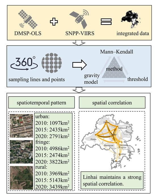
Taizhou City encompasses three distinct geographical categories: urban, urban–rural fringe, and rural areas. The urban–rural fringe region serves as a transitional zone bridging the gap between urban and rural environments. It differs from the other two categories in terms of population, economic activity, and other factors. This study employs nighttime light data to capture the distinctive activity patterns across these various zones. To ensure the validity of different nighttime lighting data, DSMP-OLS and SNPP-VIRSS and integrated data were used in this study. The characterization of different regions is achieved through key indicators such as nighttime light brightness, light fluctuation, and composite feature values. A dataset of 360 sampling lines and 9841 sampling points was established, allowing for the delineation of boundaries between urban and rural fringe areas using a combination of threshold methods and an enhanced Mann–Kendall detection algorithm [60,61,62]. To comprehensively analyze the dynamics of these fringe areas, an attraction model is employed to assess the gravitational pull exerted by these zones in 2010, 2015, and 2020 [63]. This model facilitates the examination of spatial and temporal variations and interactions among the fringe areas (Figure 2).
3.2. Formulation of a Model for Urban–Rural Fringe Identification
3.2.1. Quantification of Standardized Light Intensity Fluctuations
Due to a certain level of oversaturation in nighttime lighting data, it becomes challenging to capture the decay pattern of light brightness as it diminishes from urban to rural areas. Drawing from a series of studies, it was observed that areas with higher light brightness values are more likely to be classified as urban, while the opposite holds true for rural areas [64,65]. Given the urban fringe’s role as a transitional zone between urban and rural landscapes, it becomes crucial to accurately distinguish the light luminance disparities between the urban fringe area and its adjacent surroundings. To achieve this, it is necessary to calculate the changes in light luminance within a defined range. Therefore, this study employs the degree of nighttime lamp luminance undulation as a basis for demarcating the boundary between the city and the fringe area. The nighttime light luminance undulation degree quantifies the degree of change within a specific unit by computing the difference between the maximum and minimum luminance values within the unit’s vicinity. The calculation formula is as follows:
where DNw indicates the nighttime light intensity fluctuation of a unit, and DNmax and DNmin are the maximum and minimum values of nighttime light intensity in a unit’s 3 × 3 field, respectively.
Referring to the related research, in order to eliminate the influence of different index units, we adopt the standardization treatment to standardize the nighttime lighting intensity, DN, and lighting intensity fluctuation, DNw [66]. We refer to the following formula:
where DNn is the standardized value of lighting intensity, and DN is the value of lighting intensity. DNmax and DNmin are the maximum and minimum values of nighttime lighting intensity. DNwn is the standardized value of lighting luminance undulation, and DNwmax and DNwmin are the maximum and minimum values of nighttime lighting intensity fluctuation in the study area, respectively. Referring to the research results obtained by Feng et al. [34], the distribution of the boundaries is adjusted with 0.01 as the adjustment amplitude, and after several attempts, the distribution of the boundaries is shown to present a closed area. The thresholds for the boundary of the fringe areas in 2010, 2015, and 2020 are finally determined, and the finalized thresholds are 0.39, 0.38, and 0.32, respectively (Figure 3).
3.2.2. Constructing the Formula for the Composite Light Characteristics Value
For the boundary between the urban fringe area and the rural area, we use the coordination degree formula to construct the characteristic combination value of nighttime lighting intensity fluctuation [67]. The calculation formula is as follows:
where C is the characteristic combination value of nighttime lighting intensity fluctuation, DNn is the normalized value of nighttime lighting intensity for cell n, and DNwn is the normalized value of nighttime lighting intensity fluctuation.
In the ArcGIS 10.6 software, the nighttime lighting intensity, nighttime lighting intensity fluctuation, and combination values were calculated for Taizhou in 2010, 2015, and 2020 (Figure 4).
3.2.3. Determination of Boundary Range through Adjusted Mann–Kendall Threshold Test
Building upon the feature combination values of nighttime light intensity, our aim is to enhance the precision in identifying the boundary transition points of the urban–rural fringe area. To achieve this, we seek to identify recurring patterns within the feature combination values and pinpoint the breakpoints by strategically placing sampling points. We adopt the city hall as the central reference point, establishing the east direction as 0°. Subsequently, we position sampling lines at 1° intervals, resulting in a total of 360 profile lines spanning Taizhou. Resampling at 1° intervals can be carried out in a way that ensures a uniform distribution of sampling points without affecting the computational efficiency. The implementation of this process is carried out in Python, running the script in the Arcpy module of ArcGIS. Concurrently, a spatial grid with a scale of 1 km is meticulously created within the study area, aligning with the spatial resolution of the nighttime lighting data. The profile line layer is then superimposed onto the grid, allowing us to identify the sampling points at the intersections of the profile lines and the grid. This meticulous approach yielded a total of 9841 sampling points (Figure 5).
To determine the breakpoints, we extracted the combined values of nighttime light from the sampling points along each sampling line. We then developed a mutation detection model, drawing inspiration from the Mann–Kendall nonparametric test algorithm [68,69,70]. Initially employed in climate diagnosis and prediction research, the Mann–Kendall test has gained widespread usage in detecting trends within sequences. The Mann–Kendall test is known as a non-parametric test method, and the MK mutation detection method has the advantages of not requiring samples to follow a certain distribution and not being affected by a few outliers; these advantages make it more suitable for type and order variables [38]. The Mann–Kendall-inspired algorithm is expressed in the following equation:
Di and Dj represent the DN values of two neighboring points in the quantile curve. The number of points in one quantile curve is n. The operator, “E”, is the antonomasia of calculating the average value; the operator, “Var”, is the antonomasia of calculating variance. The forward sequence UFk was computed by the formulas listed above with the input DN values ranking according to the percentile from 0 to 100, while the inverse sequence UBk was computed in the same way using the inverse DN values ranking according to the percentile from 100 to 0 as input. The mutation point of the original data was obtained by finding the intersection point of the forward and inverse sequences on the same abscissa.
In the interest of enhancing the computational efficiency, this study builds upon the Mann–Kendall algorithm and further optimizes the calculation of mutation points for each profile line. The formula for this optimized process is as follows:
where Dij is the absolute difference of the combined value of the feature group of the jth point on the ith sampling line, and Cij, Cij−1, and Cij+1 are the combined values of the features of the jth, j−1, and j+1 sampling points on the ith sampling line. And Si is the critical threshold value of the breakpoint on the ith sampling line. When Dij is larger than Si, then Dij is labeled as the breakpoint of this sampling line. The absolute difference change curves for the years 2010 and 2020 were produced using the four sampling lines of 0°, 90°, 180°, and 270° as representatives (Figure 6). The dashed line represents the critical threshold of the mutation point for that year, and the points above the dashed line represent the breakpoints on this sampling line. In order to exclude the influence of anomalies on boundary confirmation, sampling points located at the tail end of the sampling line at the administrative boundary and some dispersed anomalies were excluded. The removal of breakpoints was primarily considered from the following perspectives. Firstly, some isolated points were scattered in small areas, failing to form closed regions with neighboring points. Secondly, certain abrupt points were distributed along the boundaries of the study area, which did not align with the understanding of peri-urban areas. Lastly, there were some clustered points, and the removal aimed to eliminate nearby interfering points to clarify connections with adjacent points. Based on these considerations, the removal of certain abrupt points was implemented. Breakpoints were ultimately achieved at the outer fringe boundary for both years (Figure 7). The map of the urban–rural fringe area of Taizhou was obtained by connecting the breakpoints in a smooth order and making some corrections.
3.3. Spatial Correlation Measurement of Urban–Rural Fringe
The urban fringe area is influenced by the surrounding neighboring regions, and the interconnectedness among these regional units contributes to the distinct roles played by various areas, resulting in varying spatial configurations of the fringe area at different times. To delve into the formation mechanisms and spatial relationships within the fringe area, we employ the gravitational calculation method to quantify the spatial forces exerted within the fringe area. The gravity model is grounded in the principle of distance attenuation, drawing inspiration from the laws of physics governing gravity. It is extensively applied in the analysis of spatial interactions [71,72,73]. The calculation expression for this model is as follows:
where Gij denotes the spatial correlation between region i and region j, indicating the degree of association strength between these two regions; K is the gravitational constant, which takes the value of 1; Qi and Qj are the masses of region i and region j, respectively; dij is the distance between region i and region j; and r is the friction coefficient, which is usually affected by the quality of the transportation network, the smoothness of the information network, and other accessibility constraints such as the transportation modes in the region. According to the summary of established research cases, the determination of the r value needs to consider the research scale and traffic smoothness comprehensively [74,75]. In this study, the friction coefficient, r, is set to 2, taking into account the spatial scale of Taizhou and the conditions of the transportation network. Traditional spatial forces between regions are often characterized by assessing the overall attributes of a specific region, which typically involve indicators like population or economy. However, these traditional approaches tend to overlook the broader developmental factors that influence regions, including aspects related to information, culture, and science and technology. Consequently, this approach results in an incomplete representation of a city’s overall quality. To address this limitation, this study recognizes that nighttime light intensity can offer a comprehensive reflection of various aspects, such as economy, population, and industrial activity. Furthermore, it serves as an effective indicator of the level of urbanization. Consequently, this study employs the summation of light intensity values within the urban and rural fringe areas as a proxy for assessing the quality of the region.
The spatial distance between regions reflects the probability trend of gravitational interaction and spatial association among regions. It encompasses a comprehensive distance calculation that takes into account transportation and road network factors. Therefore, it is not appropriate to directly employ the straight-line distance between two regions to determine the magnitude of gravitational force. Considering the geographical relationship and the time cost associated with transportation within the study area, motorized driving is deemed the most efficient mode of transportation between two regions. Consequently, in this study, we employ the government sites of each district and county as the reference points for spatial force calculation. The Baidu Maps platform takes into account road conditions and road information, obtaining a more detailed road network and faster data updates. Utilizing the Baidu map data interface, we conduct batch calculations of the driving time, dij (in minutes), between different points during off-peak hours. This driving time represents the temporal distance between regions and serves as a proxy for measuring the strength of correlation among the fringe districts. The correlation between areas can be determined using nighttime light intensity and distance (Table 1).
4. Results
4.1. Analysis of Light Intensity, Degree of Light Intensity Fluctuation, and the Characteristic Combination Value
From 2010 to 2020, there were certain differences in the nighttime light intensity, light intensity fluctuation, and combination values in Taizhou City (Table 2). Spatially, the distribution appeared concentrated and contiguous, with areas of higher light intensity concentrated at the junction of Jiaojiang, Huangyan, and Luqiao. Regions with light intensity values greater than 50 were identified as high-value areas, and the percentage of the total area they covered was used to characterize the urban activity rate (UC). Over the span of 10 years, the range of nighttime light intensity showed minimal variation, but the mean values increased, indicating an increase in the dispersion of data and an improvement in urban activity. This suggests an overall development of the city from a clustered local development pattern to a multi-core synchronous development model. The fluctuation in nighttime light intensity was used as an indicator to define urban and peri-urban areas. After standardization, grid units with brightness fluctuation values greater than 0.39, 0.38, and 0.32 were selected as the boundary lines for urban and peri-urban areas in 2010, 2015, and 2020, respectively. The change in nighttime light intensity feature combination values effectively distinguished peri-urban and rural areas. The Mann–Kendall modified algorithm was applied to calculate the absolute differences in the feature combination values, representing the abrupt points on the outer boundary of peri-urban areas. In the east direction, the breakpoints in 2010, 2015, and 2020 were located at distances of 1 km, 3 km, and 5 km from the city hall, respectively. In the northward and westward directions, a similar overall trend was observed, with three distinct abrupt regions. In the southward direction, the absolute difference curves for all three years exhibited significant fluctuations, indicating a pronounced urban development and evident urban integration in this direction.
Over the course of the decade, there has been a discernible increase in nighttime light intensity in Taizhou City. The number of high-intensity areas with light intensity values greater than 50 has experienced a substantial increase, growing by a factor of 7.69. The overall fluctuation in nighttime light intensity has increased, signifying heightened activity in various illuminated regions within the study area, resulting in larger fluctuations compared to the surrounding areas. However, the disparity in fluctuation between the urban and fringe areas has somewhat diminished. This indicates the emergence of multiple high-intensity activity zones within the study area, contributing to larger fluctuations, while simultaneously revealing a trend of reduced disparity between the city center and peri-urban areas, suggestive of a certain level of integration. To address smaller fragmented areas and provide a more intuitive representation of the spatiotemporal changes in fringe regions, fragmented areas are consolidated with adjacent regions.
4.2. Spatiotemporal Pattern of Urban–Rural Fringe Areas
Following the delineation thresholds for nighttime light intensity, fluctuations, and combination values, Taizhou City is classified into urban, urban–rural fringe, and rural regions. Urban areas covered 10.91%, 24.22%, and 39.42% of the total area in 2010, 2015, and 2020, respectively, showing a notable growth trend. Specifically, from 2010 to 2015, 1382 km2 of fringe areas transitioned to urban, while 131 km2 of rural areas became fringe areas. Between 2015 and 2020, 508 km2 of fringe areas transformed into urban areas, and 1691 km2 of rural areas shifted to fringe areas. In a comprehensive analysis, it becomes evident that urban areas are characterized by a discernible trend of expansion, whereas fringe areas display dynamic fluctuations. The delineation between fringe and rural areas introduces a nuanced layer of ambiguity and uncertainty within the classification framework (Figure 8).
In terms of spatial distribution, the urban development process led urban areas to expand into adjacent regions. Notably, the confluence of Huangyan, Jiaojiang, Wenling, and Luqiao at their borders formed contiguous urban areas, fostering integration with Yuhuan. Urban expansion was observed in Xianju, Tiantai, Linhai, and Sanmen; however, this did not culminate in a concentrated distribution, as would be expected in a typical urban development scenario (Figure 9).
At the county level, over the decade, fringe areas around Luqiao, Jiaojiang, and Huangyan central districts decreased, while urban areas grew by 115 km2, 85 km2, and 80 km2. Wenling, Yuhuan, and Linhai experienced significant urban growth, expanding by 615 km2, 308 km2, and 307 km2, respectively, influenced by their central districts. Tiantai and Xianju had slight urban area expansions, with minimal changes in region categories. In contrast, Sanmen showed rapid urban development, with urban and peri-urban areas increasing by 74 km2 and 257 km2, while the rural areas decreased by 331 km2 (Table 3).
4.3. Spatial Correlation Intensity in Urban–Rural Fringe Areas
In Taizhou City, the strength of spatiotemporal correlations in urban–rural fringe areas among different counties varies due to factors such as economic development, road accessibility, and information flow (Figure 10). By employing the Jenks method by Arcgis, we categorized the spatial correlation strength into five levels. Spatially, in both 2010 and 2015, the correlation strength exhibited similarities in both years, forming a radiating structure centered around Linhai. The maximum spatial correlation strengths were 15,994 and 9741, respectively, located between Huangyan and Linhai. Huangyan, as the central urban area, with developed transportation and industry, strongly attracts nearby regions. Linhai, adjacent to Huangyan, is a primary area for urban expansion due to its favorable location and transportation. It also accommodates urban–rural fringe areas, supporting industrial development from the central urban area. Strong spatial correlations exist between Linhai and Wenling, as well as between Linhai and Xianju. Conversely, Luqiao, a smaller central urban area, has weaker spatial attraction but forms localized correlation networks in nearby regions due to lower time–distance costs. Linhai and Huangyan emerge as areas with the strongest spatial attraction, concentrated around the central urbanized zone, with significant transportation advantages and higher spatial correlation strengths with adjacent regions. In contrast, Tiantai, Yuhuan, and Sanmen exhibit relatively weaker spatial correlation strengths.
The spatial correlation intensity of each region exhibits some changes in different periods. In 2020, the spatial correlation intensity displays a radial structure centered around Linhai, encompassing Xianju, Tiantai, and Sanmen. There is a notable increase in spatial attraction among these four regions compared to 2010. The highest spatial association strength recorded is 448,148, observed between Linhai and Xianju. However, there are some differences. The triangular network with Luqiao as the sub-center observed in 2010 disappears, and the association intensity between Jiaojiang, Luqiao, Yuhuan, and Wenling decreases. Among these, the Yuhuan–Luqiao region exhibits the lowest spatial association at 75. In terms of administrative units, Linhai, Tiantai, and Sanmen stand out as the three most spatially attractive areas. These three districts retain substantial amounts of fringe areas with considerable potential for future development. Conversely, Yuhuan, Luqiao, and Wenling exhibit weaker spatial attractiveness. The fringe areas of these three regions have gradually transformed into urban areas over the course of 10 years of development and integration. This reduction in undeveloped area has resulted in decreased spatial association with other regions. Additionally, Yuhuan’s location in the southernmost part of the city results in higher transportation time costs when connecting with other regions, contributing to a decrease in its spatial attractiveness to some extent.
5. Discussion
5.1. Error Analysis
Using long-term nighttime light data at the city scale can provide a better understanding of the spatial development patterns of urban areas. To validate the level and variation of urbanization in Taizhou City, the urban population percentage from the statistical yearbook was used to represent the urbanization rate. This served as the benchmark for conducting error analysis in this study. The spatial urbanization rate was characterized by the ratio of the sum of urban and fringe areas to the total area. From 2010 to 2020, the population urbanization rate increased from 55.54% to 61.98%, and the spatial urbanization rate increased from 60.52% to 65.79%. The absolute errors were 4.98% and 3.81%, respectively. Furthermore, based on land use from remote sensing images, three regions, A, B, and C, in 2020 were selected for validation and comparison, aligning with distinct image characteristics in different areas (Figure 11). Based on data from the statistical yearbooks of 2010 and 2020, alongside findings from the second and third national land surveys, the urban population is projected to increase from 3.32 million in 2010 to 4.10 million in 2020. Correspondingly, the urban land area is anticipated to expand from 850 km2 to 1080 km2 during the same period, reflecting growth rates of 23.81% for the urban population and 27.05% for urban land. A long-term time series analysis revealed a similar trend in the spatial urbanization rate to the population urbanization rate in Taizhou. Due to the spatial resolution of nighttime light data and the influence of identification boundary thresholds, scattered urban patches were merged into contiguous areas during the spatial recognition process, leading to an enlargement in the spatial recognition scope for urban and peri-urban areas. Additionally, imaging errors such as light pixel overflow, background noise, and interference from other light sources occurred during different years [76]. It is worth noting that the aerosol optical depth (AOD) during the imaging process significantly influences nighttime light data, and there is a pronounced spatial coherence between the two variables. [77,78,79,80]. By drawing on the research of other scholars [81], a spatiotemporal distribution map of PM2.5 concentration was generated to support the results of this study (Figure 12).
5.2. Limitations and Prospects
The night light data, transcending constraints such as administrative demarcations and data acquisition limitations, offer a comprehensive reflection of activities associated with population, transportation, and industry. These data serve as a metric for gauging the overall developmental status and urban vibrancy across diverse regions. Past scholars have harnessed nocturnal light data to investigate parameters like population density and built-up areas, presenting potential avenues for identifying urban–rural fringe areas across distinct temporal periods [82,83]. However, this study faces several limitations and challenges. Firstly, there is inherent uncertainty and unknowns in the data. The relationship between nighttime light data and various indicators of urbanization development requires quantitative estimation. By incorporating additional auxiliary data such as land use, road networks, and topography, and by employing regression statistical analysis and methods like random forest, the relationship between nighttime light data and economic output can be cross-validated and evaluated [84]. A clearer quantitative relationship can partially address the uncertainty in nighttime light data. Future research efforts may consider adopting more rigorous statistical methods and models to construct a clearer relationship between nighttime light data and the comprehensive state of urban development. Secondly, the method for determining the spatial threshold of urban–rural fringe areas in this study relies on manual interpretation. The use of threshold detection methods and the removal of pseudo-breakpoints at the urban scale to depict fringe areas introduce certain limitations. Utilizing scientific algorithms such as adaptive thresholds and machine learning can effectively avoid uncertainties arising from subjective human experience [85]. In the era of flourishing big data, a wealth of data from multiple sources provides conditions for enhancing resolution speed and computational accuracy. By combining advanced specialized algorithm models, including deep learning and artificial intelligence, for simulation computing, the potential of obtaining heterogeneous data from multiple sources can be fully exploited [86]. Supported by foundational data, the effective selection of data and optimization of algorithm models and the elimination of both internal and external errors in the system become critical directions for future exploration and in-depth research.
Applying the gravity model, we calculate the interaction relationships between peri-urban areas, transforming different element flows into regional-scale and distance-based relationships. The gravity model not only provides an intuitive representation of the spatial connections between regions but also quantifies these connections, measuring the strength of interaction between regions. This approach encapsulates the elements of the study within an abstract model, simplifying various factors through a comprehensive indicator like mass, thereby facilitating the calculation of attraction relationships between regions. With the evolution of geographic big data, possibilities arise from various data sources, such as geospatial data, mobile signaling, and media check-in data, to explore the interactions among different flow elements [87,88,89]. Establishing relationships between different flow elements and gravity models within the vast and heterogeneous dataset is a key focus for future research. Furthermore, due to the uncertainty in the costs associated with logistics, human mobility, and information transmission, the model simplifies calculations by substituting driving time for the distance in the gravity model. By combining topological information from road networks and other transportation big data, a nuanced assessment of the transmission costs for various flow elements can be conducted. Performing precise calculations of spatial interactions under different traffic scenarios provide a promising avenue for future research in this emerging field.
6. Conclusions
Exploring the spatial evolution pattern of urban areas in Taizhou City using nighttime light data reveals notable trends. From 2010 to 2020, the average nighttime light intensity increased by 2.10 times, and the urban area expanded gradually from 1097 km2 to 2791 km2, demonstrating a trend of continuous expansion and integration with the fringe areas. Conversely, the fringe areas experienced an evolution pattern characterized by initial contraction followed by expansion. In terms of spatial patterns, the gradual fusion of the central urban areas in Jiaojiang, Luqiao, and Huangyan formed a concentrated and contiguous urban region, influencing the adjacent areas of Wenling and Yuhuan. Concerning spatial forces, Linhai, with its favorable transportation conditions and extensive fringe areas, exerts strong attraction to the fringe areas of other regions. As the integration of central urban areas progresses and available development space diminishes, the attractiveness to fringe areas in other regions shows a declining trend.
The findings of this research demonstrate the practicality and reliability of using nighttime light data to uncover the spatial and temporal changes in urban fringe areas. Additionally, this study offers a methodological framework for assessing the strength of spatial associations in regional-scale fringe areas, providing a quantitative foundation for urban spatial planning and future regional development.
Author Contributions
B.F. and B.X. designed the study. B.F. processed the data and drafted the paper. All authors have read and agreed to the published version of the manuscript.
Funding
This study was funded by the National Natural Science Foundation of China (41971166), Chinese Academy of Sciences (CAS) Program of Young Scholar for Regional Development (2021-003) and German Federal Ministry of Education and Research for the Sustainable Development of Urban Areas “Urban-Uural Assembly” (01LE1804A1).
Data Availability Statement
The nighttime light data for the years 2010, 2015, and 2020 are sourced from Harvard Dataverse (https://dataverse.harvard.edu/dataset.xhtml?persistentId=doi:10.7910/DVN/GIYGJU). Other data presented in this study are available upon request from the corresponding author.
Conflicts of Interest
The authors declare no conflict of interest.
References
- Lang, W.; Chen, T.; Li, X. A new style of urbanization in China: Transformation of urban rural communities. Habitat Int. 2016, 55, 1–9. [Google Scholar] [CrossRef]
- Tian, Y.; Qian, J.; Wang, L. Village classification in metropolitan suburbs from the perspective of urban-rural integration and improvement strategies: A case study of Wuhan, central China. Land Use Policy 2021, 111, 105748. [Google Scholar] [CrossRef]
- Ding, W.; Chen, H. Urban-rural fringe identification and spatial form transformation during rapid urbanization: A case study in Wuhan, China. Build. Environ. 2022, 226, 109697. [Google Scholar] [CrossRef]
- Yang, Y.; Bao, W.; Wang, Y.; Liu, Y. Measurement of urban-rural integration level and its spatial differentiation in China in the new century. Habitat Int. 2021, 117, 102420. [Google Scholar] [CrossRef]
- Zhu, J.; Lang, Z.; Yang, J.; Wang, M.; Zheng, J.; Na, J. Integrating spatial heterogeneity to identify the urban fringe area based on NPP/VIIRS nighttime light data and dual spatial clustering. Remote Sens. 2022, 14, 6126. [Google Scholar] [CrossRef]
- Lopez-Goyburu, P.; García-Montero, L. The urban-rural interface as an area with characteristics of its own in urban planning: A review. Sustain. Cities Soc. 2018, 43, 157–165. [Google Scholar] [CrossRef]
- Thwaites, K.; Simpson, J.; Simkins, I. Transitional edges: A conceptual framework for socio-spatial understanding of urban street edges. Urban Des. Int. 2020, 25, 295–309. [Google Scholar] [CrossRef]
- Ann, T.; Wu, Y.; Zheng, B.; Zhang, X.; Shen, L. Identifying risk factors of urban-rural conflict in urbanization: A case of China. Habitat Int. 2014, 44, 177–185. [Google Scholar]
- Amirinejad, G.; Donehue, P.; Baker, D. Ambiguity at the peri-urban interface in Australia. Land Use Policy 2018, 78, 472–480. [Google Scholar] [CrossRef]
- Banu, N.; Fazal, S. Development of infrastructural facilities in public sector on the urban fringe of Aligarh city: A regional perspective from north India. J. Infrastruct. Dev. 2013, 5, 151–168. [Google Scholar] [CrossRef]
- Gizelis, T.; Pickering, S.; Urdal, H. Conflict on the urban fringe: Urbanization, environmental stress, and urban unrest in Africa. Polit. Geogr. 2021, 86, 102357. [Google Scholar] [CrossRef]
- Fei, W.; Zhao, S. Urban land expansion in China’s six megacities from 1978 to 2015. Sci. Total Environ. 2019, 664, 60–71. [Google Scholar] [CrossRef] [PubMed]
- Peng, J.; Liu, Q.; Blaschke, T.; Zhang, Z.; Liu, Y.; Hu, Y.; Wang, M.; Xu, Z.; Wu, J. Integrating land development size, pattern, and density to identify urban-rural fringe in a metropolitan region. Landsc. Ecol. 2020, 35, 2045–2059. [Google Scholar] [CrossRef]
- Li, G.; Cao, Y.; He, Z.; He, J.; Wang, J.; Fang, X. Understanding the diversity of urban-rural fringe development in a fast urbanizing region of China. Remote Sens. 2021, 13, 2373. [Google Scholar] [CrossRef]
- Peng, J.; Hu, Y.; Liu, Y.; Ma, J.; Zhao, S. A new approach for urban-rural fringe identification: Integrating impervious surface area and spatial continuous wavelet transform. Landsc. Urban Plan. 2018, 175, 72–79. [Google Scholar] [CrossRef]
- Chen, Z.; Yu, S.; You, X.; Yang, C.; Wang, C.; Lin, J.; Wu, W.; Yu, B. New nighttime light landscape metrics for analyzing urban-rural differentiation in economic development at township: A case study of Fujian province, China. Appl. Geogr. 2023, 150, 102841. [Google Scholar] [CrossRef]
- Halder, B.; Bandyopadhyay, J.; Banik, P. Monitoring the effect of urban development on urban heat island based on remote sensing and geo-spatial approach in Kolkata and adjacent areas, India. Sustain. Cities Soc. 2021, 74, 103186. [Google Scholar] [CrossRef]
- Shao, Z.; Sumari, N.; Portnov, A.; Ujoh, F.; Musakwae, W.; Manla, P. Urban sprawl and its impact on sustainable urban development: A combination of remote sensing and social media data. Geo-Spat. Inf. Sci. 2021, 24, 241–255. [Google Scholar] [CrossRef]
- Yang, J.; Dong, J.; Sun, Y.; Zhu, J.; Huang, Y.; Yang, S. A constraint-based approach for identifying the urban-rural fringe of polycentric cities using multi-sourced data. Int. J. Geogr. Inf. Sci. 2022, 36, 114–136. [Google Scholar] [CrossRef]
- Wang, X.; Wang, D.; Lu, J.; Gao, W.; Jin, X. Identifying and tracking the urban-rural fringe evolution in the urban-rural transformation period: Evidence from a rapidly urbanized rust belt city in China. Ecol. Indic. 2023, 146, 109856. [Google Scholar] [CrossRef]
- Huang, J.; Zhou, Q.; Wu, Z. Delineating urban fringe area by land cover information entropy-An empirical study of Guangzhou-Foshan metropolitan area, China. ISPRS Int. J. Geoinf. 2016, 5, 59. [Google Scholar] [CrossRef]
- Ma, Y.; Qiao, J.; Han, D. Interpreting the humanistic space of urban-rural interface using consumption behaviors. J. Rural Stud. 2022, 93, 513–521. [Google Scholar] [CrossRef]
- Wang, Y.; Han, Y.; Pu, L.; Jiang, B.; Yuan, S.; Xu, Y. A novel model for detecting urban fringe and its expanding patterns: An application in Harbin City, China. Land 2021, 10, 876. [Google Scholar] [CrossRef]
- Long, Y.; Luo, S.; Liu, X.; Luo, T.; Liu, X. Research on the dynamic evolution of the landscape pattern in the urban fringe area of Wuhan from 2000 to 2020. ISPRS Int. J. Geoinf. 2022, 11, 483. [Google Scholar] [CrossRef]
- Yang, Y.; Ma, M.; Tan, C.; Li, W. Spatial recognition of the urban-rural fringe of Beijing using DMSP/OLS nighttime light data. Remote Sens. 2017, 9, 1141. [Google Scholar] [CrossRef]
- Dong, Q.; Qu, S.; Qin, J.; Yi, D.; Liu, Y.; Zhang, J. A method to identify urban fringe area based on the industry density of POI. ISPRS Int. J. Geoinf. 2022, 11, 128. [Google Scholar] [CrossRef]
- Surya, B.; Ahmad, D.; Sakti, H.; Sahban, H. Land use change, spatial interaction, and sustainable development in the metropolitan urban areas, South Sulawesi Province, Indonesia. Land 2020, 9, 95. [Google Scholar] [CrossRef]
- Karagoz, K.; Saray, M. Trade potential of Turkey with Asia-Pacific countries: Evidence from panel gravity model. Int. Econ. Stud. 2022, 36, 19–26. [Google Scholar]
- Ulucak, R.; Yucel, A.G.; Ilkay, S.C. Dynamics of tourism demand in Turkey: Panel data analysis using gravity model. Tour. Econ. 2020, 26, 1394–1414. [Google Scholar] [CrossRef]
- Chen, J.; Xu, C.; Li, K.; Song, M. A gravity model and exploratory spatial data analysis of prefecture-scale pollutant and CO2 emissions in China. Ecol. Indic. 2018, 90, 554–563. [Google Scholar] [CrossRef]
- Zhu, K.; Gu, Z.; Li, J. Analysis of the China’s interprovincial innovation connection network based on modified gravity model. Land 2023, 12, 1091. [Google Scholar] [CrossRef]
- Xia, N.; Cheng, L.; Chen, S.; Wei, X.; Zong, W.; Li, M. Accessibility based on gravity-radiation model and Google Maps API: A case study in Australia. J. Transp. Geogr. 2018, 72, 178–190. [Google Scholar] [CrossRef]
- Song, Y.; Wang, J.; Ge, Y.; Xu, C. An optimal parameters-based geographical detector model enhances geographic characteristics of explanatory variables for spatial heterogeneity analysis: Cases with different types of spatial data. GISci. Remote Sens. 2020, 57, 593–610. [Google Scholar] [CrossRef]
- Feng, Z.; Peng, J.; Wu, J. Using DMSP/OLS nighttime light data and K-means method to identify urban-rural fringe of megacities. Habitat Int. 2020, 103, 102227. [Google Scholar] [CrossRef]
- Wang, G.; Peng, W.; Xiang, J.; Ning, L.; Yu, Y. Modelling spatiotemporal carbon dioxide emission at the urban scale based on DMSP-OLS and NPP-VIIRS data: A case study in China. Urban Clim. 2022, 46, 101326. [Google Scholar] [CrossRef]
- Ortakavak, Z.; Cabuk, S.N.; Cetin, M.; Kurkcuoglu, M.A.S.; Cabuk, A. Determination of the nighttime light imagery for urban city population using DMSP-OLS methods in Istanbul. Environ. Monit. Assess. 2020, 192, 790. [Google Scholar] [CrossRef] [PubMed]
- Gu, Y.; Shao, Z.; Huang, X.; Cai, B. GDP forecasting model for China’s provinces using nighttime light remote sensing data. Remote Sens. 2022, 14, 3671. [Google Scholar] [CrossRef]
- Huang, Y.; Yang, J.; Chen, M.; Wu, C.; Ren, H.; Liu, Y. An approach for retrieving consistent time Series “Urban core—Suburban-rural” (USR) structure using nighttime light data from DMSP/OLS and NPP/VIIRS. Remote Sens. 2022, 14, 3642. [Google Scholar] [CrossRef]
- Li, C.; Li, G.; Tao, G.; Zhu, Y.; Wu, Y.; Li, X.; Liu, J. DMSP/OLS night-time light intensity as an innovative indicator of regional sustainable development. Int. J. Remote Sens. 2019, 40, 1594–1602. [Google Scholar] [CrossRef]
- Lv, Q.; Liu, H.; Wang, J.; Liu, H.; Shang, Y. Multiscale analysis on spatiotemporal dynamics of energy consumption CO2 emissions in China: Utilizing the integrated of DMSP-OLS and NPP-VIIRS nighttime light datasets. Sci. Total Environ. 2020, 703, 134394. [Google Scholar] [CrossRef]
- Chen, X.; Nordhaus, W.D. VIIRS nighttime lights in the estimation of cross-sectional and time-series GDP. Remote Sens. 2019, 11, 1057. [Google Scholar] [CrossRef]
- Zhang, X.; Gibson, J. Using multi-source nighttime lights data to proxy for county-level economic activity in China from 2012 to 2019. Remote Sens. 2022, 14, 1282. [Google Scholar] [CrossRef]
- Liu, Z.; Zhang, J.; Li, X.; Chen, X. Long-term resilience curve analysis of wenchuan earthquake-affected counties using dmsp-ols nighttime light images. IEEE J. Sel. Top. Appl. Earth Obs. Remote Sens. 2021, 14, 10854–10874. [Google Scholar] [CrossRef]
- Li, X.; Li, D.; Xu, H.; Wu, C. Intercalibration between DMSP/OLS and VIIRS night-time light images to evaluate city light dynamics of Syria’s major human settlement during Syrian Civil War. Int. J. Remote Sens. 2017, 38, 5934–5951. [Google Scholar] [CrossRef]
- Tan, X.; Huang, B.; Batty, M.; Li, J. Urban spatial organization, multifractals, and evolutionary patterns in large cities. Ann. Am. Assoc. Geogr. 2021, 111, 1539–1558. [Google Scholar] [CrossRef]
- Hu, X.; Qian, Y.; Pickett, S.; Zhou, W. Urban mapping needs up-to-date approaches to provide diverse perspectives of current urbanization: A novel attempt to map urban areas with nighttime light data. Landsc. Urban Plan 2020, 195, 103709. [Google Scholar] [CrossRef]
- Zhou, Y.; Li, C.; Zheng, W.; Rong, Y.; Liu, W. Identification of urban shrinkage using NPP-VIIRS nighttime light data at the county level in China. Cities 2021, 118, 103373. [Google Scholar] [CrossRef]
- Yang, Y.; Wu, J.; Wang, Y.; Huang, Q.; He, C. Quantifying spatiotemporal patterns of shrinking cities in urbanizing China: A novel approach based on time-series nighttime light data. Cities 2021, 118, 103346. [Google Scholar] [CrossRef]
- Cao, R.; Tu, W.; Yang, C.; Li, Q.; Liu, J.; Zhu, J.; Zhang, Q.; Li, Q.; Qiu, G. Deep learning-based remote and social sensing data fusion for urban region function recognition. ISPRS J. Photogramm. 2020, 163, 82–97. [Google Scholar] [CrossRef]
- Wu, Y.; Zhang, X.; Skitmore, M.; Song, Y.; Hui, E. Industrial land price and its impact on urban growth: A Chinese case study. Land Use Policy 2014, 36, 199–209. [Google Scholar] [CrossRef]
- Tang, X.; Shen, C.; Shi, D.; Cheema, S.A.; Khan, M.I.; Zhang, C.; Chen, Y. Heavy metal and persistent organic compound contamination in soil from Wenling: An emerging e-waste recycling city in Taizhou area, China. J. Hazard. Mater. 2010, 173, 653–660. [Google Scholar] [CrossRef] [PubMed]
- Elvidge, C.; Baugh, K.; Zhizhin, M.; Hsu, F. Why VIIRS data are superior to DMSP for mapping nighttime lights. Proc. Asia-Pac. Adv. Netw. 2013, 35, 62. [Google Scholar] [CrossRef]
- Peng, Y.; Zheng, R.; Yuan, T.; Cheng, L.; You, J. Evaluating perception of community resilience to typhoon disasters in China based on grey relational TOPSIS model. Int. J. Disast. Risk Re. 2023, 84, 103468. [Google Scholar] [CrossRef]
- Fienitz, M.; Siebert, R. Urban versus rural? Conflict lines in land use disputes in the urban–rural fringe region of Schwerin, Germany. Land 2021, 10, 726. [Google Scholar] [CrossRef]
- Levin, N.; Kyba, C.; Zhang, Q. Remote sensing of night lights: A review and an outlook for the future. Remote Sens. Environ. 2020, 237, 111443. [Google Scholar] [CrossRef]
- Qian, Y.; Wang, H.; Wu, J. Spatiotemporal association of carbon dioxide emissions in China’s urban agglomerations. J. Environ. Manag. 2022, 323, 116109. [Google Scholar] [CrossRef] [PubMed]
- Mohammad, P.; Goswami, A. A spatio-temporal assessment and prediction of surface urban heat island intensity using multiple linear regression techniques over Ahmedabad City, Gujarat. J. Indian. Soc. Remote. 2021, 49, 1091–1108. [Google Scholar] [CrossRef]
- Yang, K.; Sun, W.; Luo, Y.; Zhao, L. Impact of urban expansion on vegetation: The case of China (2000–2018). J. Environ. Manag. 2021, 291, 112598. [Google Scholar] [CrossRef]
- Wu, Y.; Shi, K.; Chen, Z.; Liu, S.; Chang, Z. Developing improved time-series DMSP-OLS-like data (1992–2019) in China by integrating DMSP-OLS and SNPP-VIIRS. IEEE Trans. Geosci. Remote Sens. 2021, 60, 1–14. [Google Scholar] [CrossRef]
- Zheng, Y.; Tang, L.; Wang, H. An improved approach for monitoring urban built-up areas by combining NPP-VIIRS nighttime light, NDVI, NDWI, and NDBI. J. Clean Prod. 2021, 328, 129488. [Google Scholar] [CrossRef]
- Huang, Q.; Yang, X.; Gao, B.; Yang, Y.; Zhao, Y. Application of DMSP/OLS nighttime light images: A Meta-Analysis and a systematic literature review. Remote Sens. 2014, 6, 6844–6866. [Google Scholar] [CrossRef]
- Chen, Z.; Yu, B.; Song, W.; Liu, H.; Wu, Q.; Shi, K.; Wu, J. A new approach for detecting urban centers and their spatial structure with nighttime light remote sensing. IEEE Trans. Geosci. Remote Sens. 2017, 55, 6305–6319. [Google Scholar] [CrossRef]
- Martin, W.; Pham, C. Estimating the gravity model when zero trade flows are frequent and economically determined. Appl. Econ. 2020, 52, 2766–2779. [Google Scholar] [CrossRef]
- Kii, M.; Tamaki, T.; Suzuki, T.; Nonomura, A. Estimating urban spatial structure based on remote sensing data. Sci. Rep. 2023, 13, 8804. [Google Scholar] [CrossRef] [PubMed]
- Xie, Y.; Weng, Q.; Fu, P. Temporal variations of artificial nighttime lights and their implications for urbanization in the conterminous United States, 2013–2017. Remote Sens. Environ. 2019, 225, 160–174. [Google Scholar] [CrossRef]
- Li, J.; Wang, F.; Fu, Y.; Guo, B.; Zhao, Y.; Yu, H. A Novel SUHI referenced estimation method for multicenters urban agglomeration using DMSP/OLS nighttime light data. IEEE J. Sel. Top. Appl. Earth Obs. Remote Sens. 2020, 13, 1416–1425. [Google Scholar] [CrossRef]
- Li, D.; Cao, L.; Zhou, Z.; Zhao, K.; Du, Z.; Han, K. Coupling coordination degree and driving factors of new-type urbanization and low-carbon development in the Yangtze River Delta: Based on nighttime light data. Environ. Sci. Pollut. R. 2022, 29, 81636–81657. [Google Scholar] [CrossRef] [PubMed]
- Wang, Z.; Yang, S.; Wang, S.; Shen, Y. Monitoring evolving urban cluster systems using DMSP/OLS nighttime light data: A case study of the Yangtze River Delta region, China. J. Appl. Remote Sens. 2017, 11, 046029. [Google Scholar] [CrossRef]
- Xu, P.; Lin, M.; Jin, P. Spatio-temporal dynamics of urbanization in China using DMSP/OLS nighttime light data from 1992–2013. Chin. Geogr. Sci. 2021, 31, 70–80. [Google Scholar] [CrossRef]
- Li, X.; Luo, Y.; Wu, J. Decoupling relationship between urbanization and carbon sequestration in the Pearl River Delta from 2000 to 2020. Remote Sens. 2022, 14, 526. [Google Scholar] [CrossRef]
- Yu, B.; Shi, K.; Hu, Y.; Huang, C.; Chen, Z.; Wu, J. Poverty evaluation using NPP-VIIRS nighttime light composite data at the county level in China. IEEE J. Sel. Top. Appl. Earth Obs. Remote Sens. 2015, 8, 1217–1229. [Google Scholar] [CrossRef]
- Zheng, W.S.; Run, J.Y.; Zhuo, R.R.; Jiang, Y.P.; Wang, X.F. Evolution process of urban spatial pattern in Hubei province based on DMSP/OLS nighttime light data. Chin. Geogr. Sci. 2016, 26, 366–376. [Google Scholar] [CrossRef]
- Han, R.; Cao, H.; Liu, Z. Studying the urban hierarchical pattern and spatial structure of China using a synthesized gravity model. Sci. China Earth Sci. 2018, 61, 1818–1831. [Google Scholar] [CrossRef]
- Li, L.; Sun, Z.; Long, X. An empirical analysis of night-time light data based on the gravity model. Appl. Econ. 2019, 51, 797–814. [Google Scholar] [CrossRef]
- Li, R.; Li, S.; Xie, Z. Integration development of urban agglomeration in central Liaoning, China, by trajectory gravity model. ISPRS Int. J. Geoinf. 2021, 10, 698. [Google Scholar] [CrossRef]
- Chang, D.; Wang, Q.; Xie, J.; Yang, J.; Xu, W. Research on the extraction method of urban built-up areas with an improved night light index. IEEE Geosci. Remote Sens. Lett. 2022, 19, 1–5. [Google Scholar] [CrossRef]
- Petržala, J. On the influence of aerosol extinction vertical profile in modeling of night sky radiance. J. Quant. Spectrosc. Radiat. Transf. 2023, 307, 108676. [Google Scholar] [CrossRef]
- Puschnig, J.; Wallner, S.; Schwope, A.; Näslund, M. Long-term trends of light pollution assessed from SQM measurements and an empirical atmospheric model. Mon. Not. R. Astron. Soc. 2023, 518, 4449–4465. [Google Scholar] [CrossRef]
- Kocifaj, M.; Kómar, L.; Lamphar, H.; Barentine, J.; Wallner, s. A systematic light pollution modelling bias in present night sky brightness predictions. Nat. Astron. 2023, 7, 269–279. [Google Scholar] [CrossRef]
- Kocifaj, M.; Bará, S. Diffuse light around cities: New perspectives in satellite remote sensing of nighttime aerosols. Atmos. Res. 2022, 266, 105969. [Google Scholar] [CrossRef]
- Van, D.; Hammer, M.; Bindle, L. Monthly global estimates of fine particulate matter and their uncertainty. Environ. Sci. Technol. 2021, 55, 15287–15300. [Google Scholar]
- Zhou, Y.; Smith, S.J.; Elvidge, C.D.; Zhao, K.; Thomson, A.; Imhoff, M. A cluster-based method to map urban area from DMSP/OLS nightlights. Remote Sens. Environ. 2014, 147, 173–185. [Google Scholar] [CrossRef]
- Wang, G.; Peng, W.; Zhang, L. Estimate of population density and diagnosis of main factors of spatial heterogeneity in the metropolitan scale, western China. Heliyon 2023, 9, 162855. [Google Scholar] [CrossRef] [PubMed]
- Liang, H.; Guo, Z.; Wu, J.; Chen, Z. GDP spatialization in Ningbo City based on NPP/VIIRS night-time light and auxiliary data using random forest regression. Adv. Space Res. 2020, 65, 481–493. [Google Scholar] [CrossRef]
- Sakagawa, Y.; Nakajima, K.; Ohashi, G. Vision based nighttime vehicle detection using adaptive threshold and multi-class classification. IEICE Trans. Fundam. Electron. Commun. Comput. Sci. 2019, 102, 1235–1245. [Google Scholar] [CrossRef]
- Casali, Y.; Aydin, N.; Comes, T. Machine learning for spatial analyses in urban areas: A scoping review. Sustain. Cities Soc. 2022, 85, 104050. [Google Scholar] [CrossRef]
- Fu, B.; Xiao, X.; Li, J. Big Data-Driven Measurement of the service capacity of public toilet facilities in China. Appl. Sci. 2022, 12, 4659. [Google Scholar] [CrossRef]
- Xue, B.; Xiao, X.; Li, J. Identification method and empirical study of urban industrial spatial relationship based on POI big data: A case of Shenyang City, China. Geogr. Sustain. 2020, 1, 152–162. [Google Scholar] [CrossRef]
- Xue, B.; Xiao, X.; Li, J.; Zhao, B.; Fu, B. Multi-source data-driven identification of urban functional areas: A case of Shenyang, China. Chin. Geogr. Sci. 2023, 33, 21–35. [Google Scholar] [CrossRef]
Figure 1.
Location of the study area.

Figure 2.
Flowchart of proposed method.

Figure 3.
Boundary line between urban and urban–rural fringes in 2010 (a), 2015 (b), and 2020 (c).

Figure 4.
Light intensity (a), intensity fluctuation (b), and combination value (c) in 2010; light intensity (d), intensity fluctuation (e), and combination value (f) in 2015; light intensity (g), intensity fluctuation (h), and combination value (i) in 2020 (the brightness of the image represents the values).

Figure 5.
Schematic diagram of 1-degree sampling line and 1 km sampling point intervals (the red dot is the location of the city hall).
Figure 5.
Schematic diagram of 1-degree sampling line and 1 km sampling point intervals (the red dot is the location of the city hall).

Figure 6.
Graph of absolute difference of 0 (a), 90 (b), 180 (c), and 270 (d) degree sampling lines.
Figure 6.
Graph of absolute difference of 0 (a), 90 (b), 180 (c), and 270 (d) degree sampling lines.

Figure 7.
The breakpoints at the boundary between urban–rural fringes and rural areas (a) with removed outliers (b) in 2010; the breakpoints at the boundary between urban–rural fringes and rural areas (c) with removed outliers (d) in 2015; the breakpoints at the boundary between urban–rural fringes and rural areas (e) with removed outliers (f) in 2020.

Figure 8.
Schematic of urban, urban–rural fringe, and rural transformation relationships (the numbers represent the areas of three types of regions, measured in square kilometers).
Figure 8.
Schematic of urban, urban–rural fringe, and rural transformation relationships (the numbers represent the areas of three types of regions, measured in square kilometers).

Figure 9.
Schematic of spatial distribution in urban, urban–rural fringe, and rural areas for 2010 (a), 2015 (b), and 2020 (c).
Figure 9.
Schematic of spatial distribution in urban, urban–rural fringe, and rural areas for 2010 (a), 2015 (b), and 2020 (c).

Figure 10.
Spatial correlation strength schematic among urban–rural fringe areas in different counties for 2010 (a), 2015 (b), and 2020 (c). (Numerical values indicate spatial attractiveness between different regions, where thicker lines and darker colors signify stronger gravitational forces).
Figure 10.
Spatial correlation strength schematic among urban–rural fringe areas in different counties for 2010 (a), 2015 (b), and 2020 (c). (Numerical values indicate spatial attractiveness between different regions, where thicker lines and darker colors signify stronger gravitational forces).

Figure 11.
Comparative analysis of urban, urban–rural fringe, and rural areas in 2020 (A–C inquire about urban, urban-rural fringe and rural validation areas, respectively).
Figure 11.
Comparative analysis of urban, urban–rural fringe, and rural areas in 2020 (A–C inquire about urban, urban-rural fringe and rural validation areas, respectively).

Figure 12.
Spatial distribution of average PM2.5 concentrations in 2010 (a), 2015 (b), and 2020 (c).
Figure 12.
Spatial distribution of average PM2.5 concentrations in 2010 (a), 2015 (b), and 2020 (c).


Table 1.
Table of regional correlation statistics.
| Point i | Qi_2010 | Qi_2015 | Qi_2020 | Point j | Qj_2010 | Qj_2015 | Qj_2020 | dij | Gij_2010 | Gij_2015 | Gij_2020 |
|---|---|---|---|---|---|---|---|---|---|---|---|
| Linhai | 10,595 | 16,284 | 8894 | Xianju | 3430 | 6880 | 2420 | 50 | 14,536.34 | 44,813.57 | 8609.39 |
| Linhai | 10,595 | 16,284 | 8894 | Tiantai | 3647 | 8620 | 1968 | 58 | 11,486.32 | 41,726.54 | 5203.15 |
| Linhai | 10,595 | 16,284 | 8894 | Sanmen | 2629 | 8357 | 1987 | 60 | 7737.29 | 37,801.50 | 4908.99 |
| Huangyan | 3774 | 3761 | 2738 | Linhai | 10,595 | 16,284 | 8894 | 50 | 15,994.21 | 24,497.65 | 9740.71 |
| Sanmen | 2629 | 8357 | 1987 | Tiantai | 3647 | 8620 | 1968 | 68 | 2073.52 | 15,579.01 | 845.68 |
| Tiantai | 3647 | 8620 | 1968 | Xianju | 3430 | 6880 | 2420 | 82 | 1860.38 | 8819.99 | 708.29 |
| Jiaojiang | 2989 | 1878 | 559 | Linhai | 10,595 | 16,284 | 8894 | 64 | 7731.56 | 7466.15 | 1213.81 |
| Huangyan | 3774 | 3761 | 2738 | Sanmen | 2629 | 8357 | 1987 | 66 | 2277.74 | 7215.49 | 1248.95 |
| Huangyan | 3774 | 3761 | 2738 | Tiantai | 3647 | 8620 | 1968 | 68 | 2976.60 | 7011.21 | 1165.31 |
| Huangyan | 3774 | 3761 | 2738 | Jiaojiang | 2989 | 1878 | 559 | 34 | 9758.21 | 6110.00 | 1324.00 |
| Linhai | 10,595 | 16,284 | 8894 | Wenling | 7807 | 2054 | 5484 | 75 | 14,704.92 | 5946.19 | 8671.06 |
| Huangyan | 3774 | 3761 | 2738 | Xianju | 3430 | 6880 | 2420 | 67 | 2883.68 | 5764.24 | 1476.04 |
| Huangyan | 3774 | 3761 | 2738 | Luqiao | 1965 | 830 | 118 | 25 | 11,865.46 | 4994.61 | 516.93 |
| Sanmen | 2629 | 8357 | 1987 | Xianju | 3430 | 6880 | 2420 | 115 | 681.85 | 4347.54 | 363.59 |
| Linhai | 10,595 | 16,284 | 8894 | Luqiao | 1965 | 830 | 118 | 57 | 6407.87 | 4159.96 | 323.02 |
| Huangyan | 3774 | 3761 | 2738 | Wenling | 7807 | 2054 | 5484 | 53 | 10,489.01 | 2750.12 | 5345.39 |
| Jiaojiang | 2989 | 1878 | 559 | Sanmen | 2629 | 8357 | 1987 | 80 | 1227.83 | 2452.26 | 173.55 |
| Jiaojiang | 2989 | 1878 | 559 | Tiantai | 3647 | 8620 | 1968 | 87 | 1440.20 | 2138.77 | 145.34 |
| Jiaojiang | 2989 | 1878 | 559 | Xianju | 3430 | 6880 | 2420 | 87 | 1354.51 | 1707.05 | 178.73 |
| Tiantai | 3647 | 8620 | 1968 | Wenling | 7807 | 2054 | 5484 | 102 | 2736.65 | 1701.80 | 1037.34 |
| Sanmen | 2629 | 8357 | 1987 | Wenling | 7807 | 2054 | 5484 | 104 | 1897.61 | 1587.03 | 1007.46 |
| Jiaojiang | 2989 | 1878 | 559 | Wenling | 7807 | 2054 | 5484 | 50 | 9334.05 | 1542.96 | 1226.22 |
| Luqiao | 1965 | 830 | 118 | Wenling | 7807 | 2054 | 5484 | 35 | 12,523.07 | 1391.69 | 528.25 |
| Jiaojiang | 2989 | 1878 | 559 | Luqiao | 1965 | 830 | 118 | 35 | 4794.60 | 1272.44 | 53.85 |
| Wenling | 7807 | 2054 | 5484 | Xianju | 3430 | 6880 | 2420 | 107 | 2338.90 | 1234.30 | 1159.16 |
| Linhai | 10,595 | 16,284 | 8894 | Yuhuan | 3776 | 579 | 4841 | 90 | 4939.10 | 1164.00 | 5315.54 |
| Luqiao | 1965 | 830 | 118 | Sanmen | 2629 | 8357 | 1987 | 84 | 732.14 | 983.04 | 33.23 |
| Luqiao | 1965 | 830 | 118 | Tiantai | 3647 | 8620 | 1968 | 87 | 946.80 | 945.25 | 30.68 |
| Luqiao | 1965 | 830 | 118 | Xianju | 3430 | 6880 | 2420 | 87 | 890.47 | 754.45 | 37.73 |
| Wenling | 7807 | 2054 | 5484 | Yuhuan | 3776 | 579 | 4841 | 55 | 9745.20 | 393.15 | 8776.21 |
| Huangyan | 3774 | 3761 | 2738 | Yuhuan | 3776 | 579 | 4841 | 75 | 2533.44 | 387.13 | 2356.38 |
| Tiantai | 3647 | 8620 | 1968 | Yuhuan | 3776 | 579 | 4841 | 116 | 1023.41 | 370.91 | 708.02 |
| Sanmen | 2629 | 8357 | 1987 | Yuhuan | 3776 | 579 | 4841 | 117 | 725.19 | 353.47 | 702.69 |
| Xianju | 3430 | 6880 | 2420 | Yuhuan | 3776 | 579 | 4841 | 122 | 870.17 | 267.64 | 787.10 |
| Jiaojiang | 2989 | 1878 | 559 | Yuhuan | 3776 | 579 | 4841 | 73 | 2117.93 | 204.05 | 507.81 |
| Luqiao | 1965 | 830 | 118 | Yuhuan | 3776 | 579 | 4841 | 80 | 1159.35 | 75.09 | 89.26 |
Table 2.
Table of nighttime light data indicators for the years 2010, 2015, and 2020.
| Light Intensity (DN) | Light Intensity Fluctuation (DNW) | Combination Value (C) | |||||||
|---|---|---|---|---|---|---|---|---|---|
| Range | Std | Mean | Uc | Range | Std | Mean | Std | Mean | |
| 2010 | [0, 59] | 12.86 | 8.74 | 1.80% | [0, 38] | 6.65 | 4.77 | 0.33 | 0.84 |
| 2015 | [0, 63] | 19.30 | 13.79 | 8.40% | [0, 54] | 7.07 | 9.03 | 0.37 | 0.62 |
| 2020 | [0, 63] | 20.46 | 18.35 | 13.85% | [0, 52] | 7.09 | 6.53 | 0.29 | 0.83 |
Std represents the standard deviation, and UC denotes the urban activity rate.
Table 3.
Table of urban, fringe, and rural area statistics for each county in 2010, 2015, and 2020.
| 2010 | 2015 | 2020 | |||||||
|---|---|---|---|---|---|---|---|---|---|
| Urban | Fringe | Rural | Urban | Fringe | Rural | Urban | Fringe | Rural | |
| Huangyan | 143 | 459 | 386 | 227 | 233 | 528 | 223 | 358 | 407 |
| Jiaojiang | 113 | 142 | 109 | 212 | 55 | 97 | 198 | 72 | 94 |
| Linhai | 125 | 1465 | 661 | 399 | 798 | 1054 | 432 | 1224 | 595 |
| Luqiao | 171 | 155 | 2 | 297 | 14 | 17 | 289 | 39 | 0 |
| Sanmen | 32 | 47 | 596 | 96 | 237 | 772 | 106 | 734 | 265 |
| Tiantai | 40 | 598 | 794 | 179 | 314 | 939 | 108 | 603 | 721 |
| Wenling | 288 | 774 | 12 | 672 | 290 | 112 | 903 | 162 | 9 |
| Xianju | 31 | 586 | 1383 | 105 | 355 | 1540 | 70 | 601 | 1329 |
| Yuhuan | 154 | 337 | 19 | 248 | 178 | 84 | 462 | 29 | 19 |
Unit: km2.
Disclaimer/Publisher’s Note: The statements, opinions and data contained in all publications are solely those of the individual author(s) and contributor(s) and not of MDPI and/or the editor(s). MDPI and/or the editor(s) disclaim responsibility for any injury to people or property resulting from any ideas, methods, instructions or products referred to in the content. |
© 2023 by the authors. Licensee MDPI, Basel, Switzerland. This article is an open access article distributed under the terms and conditions of the Creative Commons Attribution (CC BY) license (https://creativecommons.org/licenses/by/4.0/).
Share and Cite
MDPI and ACS Style
Fu, B.; Xue, B. Temporal and Spatial Evolution Analysis and Correlation Measurement of Urban–Rural Fringes Based on Nighttime Light Data. Remote Sens. 2024, 16, 88. https://doi.org/10.3390/rs16010088
AMA Style
Fu B, Xue B. Temporal and Spatial Evolution Analysis and Correlation Measurement of Urban–Rural Fringes Based on Nighttime Light Data. Remote Sensing. 2024; 16(1):88. https://doi.org/10.3390/rs16010088
Chicago/Turabian StyleFu, Bo, and Bing Xue. 2024. "Temporal and Spatial Evolution Analysis and Correlation Measurement of Urban–Rural Fringes Based on Nighttime Light Data" Remote Sensing 16, no. 1: 88. https://doi.org/10.3390/rs16010088
Note that from the first issue of 2016, this journal uses article numbers instead of page numbers. See further details here.