
A Machine Learning Approach for Mapping Chlorophyll Fluorescence at Inland Wetlands


1
Remote Sensing Centre, Institute of Geodesy and Cartography, 27 Modzelewskiego St., 02-679 Warszawa, Poland
2
Department of Geoinformatics, Cartography and Remote Sensing, Chair of Geomatics and Information Systems, Faculty of Geography and Regional Studies, University of Warsaw, 00-927 Warszawa, Poland
*
Author to whom correspondence should be addressed.
†
These authors contributed equally to this work.
Remote Sens. 2023, 15(9), 2392; https://doi.org/10.3390/rs15092392
Submission received: 3 April 2023
/
Revised: 27 April 2023
/
Accepted: 1 May 2023
/
Published: 3 May 2023
(This article belongs to the Special Issue Applications of Remote Sensing in Forest Management and Biodiversity Conservation)
Abstract
:Wetlands are a critical component of the landscape for climate mitigation, adaptation, biodiversity, and human health and prosperity. Keeping an eye on wetland vegetation is crucial due to it playing a major role in the planet’s carbon cycle and ecosystem management. By measuring the chlorophyll fluorescence (ChF) emitted by plants, we can get a precise understanding of the current state and photosynthetic activity. In this study, we applied the Extreme Gradient Boost (XGBoost) algorithm to map ChF in the Biebrza Valley, which has a unique ecosystem in Europe for peatlands, as well as highly diversified flora and fauna. Our results revealed the advantages of using a set of classifiers derived from EO Sentinel-2 (S-2) satellite image mosaics to accurately map the spatio-temporal distribution of ChF in a terrestrial landscape. The validation proved that the XGBoost algorithm is quite accurate in estimating ChF with a good determination of 0.71 and least bias of 0.012. The precision of chlorophyll fluorescence measurements is reliant upon determining the optimal S-2 satellite overpass time, which is influenced by the developmental stage of the plants at various points during the growing season. Finally, the model performance results indicated that biophysical factors are characterized by greenness- and leaf-pigment-related spectral indices. However, utilizing vegetation indices based on extended periods of remote sensing data that better capture land phenology features can improve the accuracy of mapping chlorophyll fluorescence.
1. Introduction
Monitoring wetland vegetation is one of the major objectives of the remote sensing of the environment due to its strong relationship with the exchange of atmospheric carbon dioxide (CO2) with land. Numerous environmental scientists have recognized chlorophyll fluorescence as a reliable indicator of a plant’s physiological state, and it is directly connected to photosynthesis [1,2,3]. ChF is the visible red and far-red light emitted by photosynthetic green plant tissues in response to photosynthetically active radiation (PAR) absorption, which occurs between 400 and 700 nm. ChF emission is characterized by two broad peaks that stretch from 650 to 800 nm in the red-edge region, with maxima at 690 nm and 740 nm [4]. Traditionally, the Fv/Fm parameter has been used to measure ChF, which is the most commonly used chlorophyll fluorescence measuring parameter worldwide [5,6]. Fv/Fm is typically measured with a pulse-amplitude modulation fluorometer using various active light sources under light-adapted or dark-adapted conditions [7]. It is a sensitive indicator of a plant’s photosynthetic performance, and lower values may signify stress or photoinhibition, as well as photosynthesis downregulation [8,9,10].
For the past few years, scientists have been able to observe and measure chlorophyll fluorescence in terrestrial ecosystems worldwide using low-resolution remote sensing images. This serves as a proxy for plant photosynthesis [11,12]. Nevertheless, recent studies on conventional ChF retrieval methods in terrestrial ecosystems are challenged by vegetation heterogeneity, seasonal dynamics, and variations in the physical environment among different ecosystems [13,14,15,16]. Algorithms attempting to extract patterns from satellite data are still being developed for retrieving and mapping ChF [17,18,19]. The latest machine learning (ML) approaches in ChF retrieval from the medium-resolution Sentinel and Landsat satellite images have been solely extended for inland and coastal waters [20,21,22,23]. Therefore, it is critical to evaluate novel ML methodologies that enable us to analyze and map the spatio-temporal distributions of plant chlorophyll fluorescence at wetlands frequently using satellite data from the Earth Observation Programme.
Wetland ecosystems are crucial for preserving Europe’s biodiversity and mitigating greenhouse gas levels by acting as carbon repositories. Proper ecosystem management of local water resources requires addressing the issue of wetland restoration. The largest and best preserved of its type in Central and Western Europe is the Biebrza Valley, extending in north-eastern Poland. Unfortunately, this region still faces serious problems in the field of water management and protection of the open fen areas [24,25]. Collecting data on the vegetation and biophysical properties of wetlands using satellite imagery is crucial, as it allows for the management of areas that are difficult or impossible to access for on-site observations. Several studies on the application of remote sensing techniques for environmental monitoring at Biebrza Wetlands have been developed [26,27,28]. Thus, finding the appropriate algorithm to estimate chlorophyll fluorescence accurately is crucial for studying the impact of stress on photosynthesis.
The aim of our study is to determine whether it is possible to use such a machine learning algorithm that is applicable to Sentinel-2 imagery to retrieve ChF data and map this biophysical indicator over wetlands. In situ measurements acquired during the growing season were evaluated and applied for retrieving ChF using a machine learning algorithm utilizing the spectral bands. These latter relations of ChF derived from the field and satellite-imagery-based retrievals were examined for cross-validation. The manuscript follows with the next analyses on (1) how the different spectral bands of Sentinel-2 contribute to the ChF model results, (2) the influence of using a machine learning method, and (3) how this study’s findings can be useful for wetland science and for mapping chlorophyll fluorescence using Earth Observation data.
2. Materials and Methods
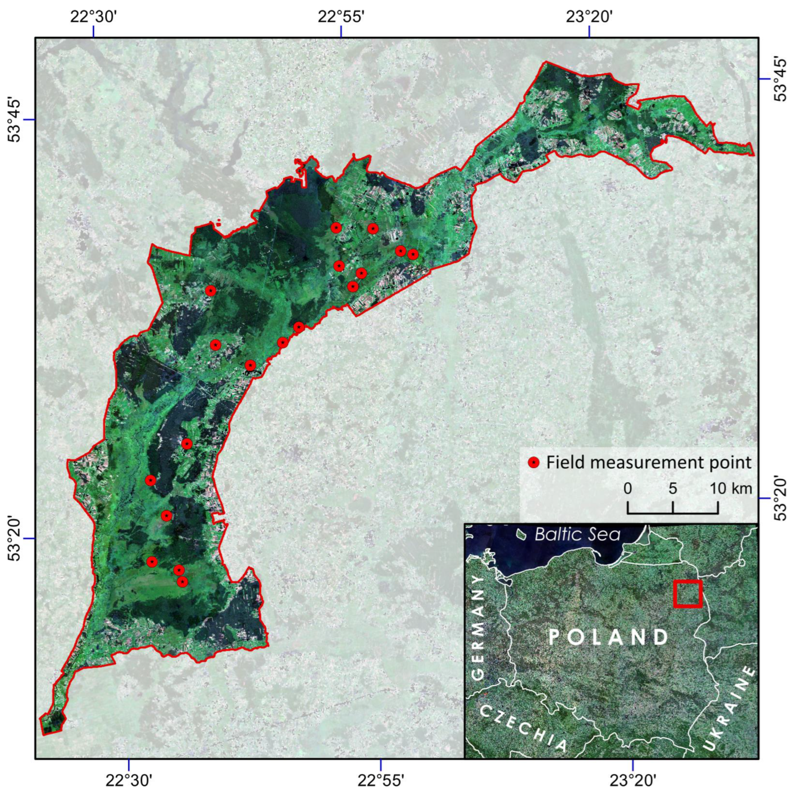
2.1. Test Site
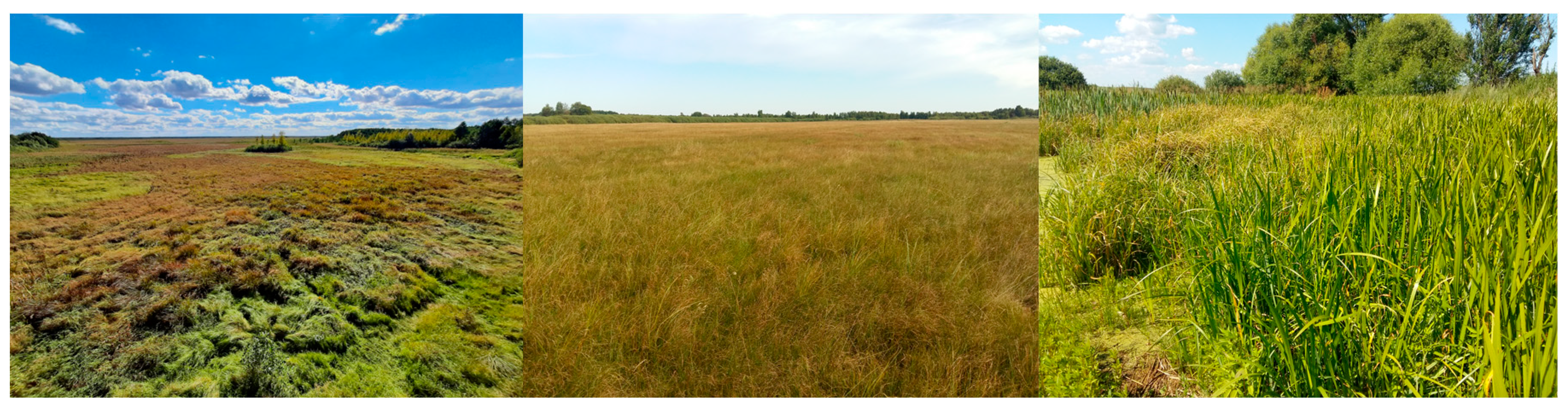
The study area is located in north-eastern Poland (Figure 2). Biebrza Wetlands is a unique ecosystem being under RAMSAR Convention for peatlands, as well as its highly diversified flora and fauna, especially reeds and sedges with grasses. The Biebrza National Park was established (in 1993) within the study area as a wetland site of global networking program NATURA 2000. The study area covers a total area of 59,223 ha of which 45% are wetlands. The area is mostly flat, with an elevation of approximately 105 m above sea level. The Biebrza River, which runs through the area, is a naturally occurring lowland river that provides a distinctive reference point for lowland valley mires and river floodplains [29]. There are approximately 70 various types of natural and semi-natural plants documented in vegetation reports [30,31]. To better understand the ecological value of wetlands, we focused on several dominant habitats, such as rush, sedge, sedge moss, and reed communities. According to the European Environment Agency’s (EEA) latest report on wetlands, certain areas of the wetlands still require restoration, particularly those that have been degraded. Our study investigated three main types of plant communities found within the wetland ecosystem: peatlands dominated by sedges, sedge mosses, and reeds (Figure 1). The research site is situated in one of the coolest regions in Poland, where the average daily air temperature throughout the year is only 6.6 °C due to the prevailing temperate continental climate. The coldest month is January, when the average air temperature is around −4.2 °C, and the warmest month is July, with an average temperature of 17.5 °C. Snow coverage usually lasts for a maximum of 140 days, and the average annual precipitation ranges from 550 to 650 mm. Additionally, the growing season in the wetlands is less than 200 days, making it one of the shortest in the country [32].
2.2. Field Measurements
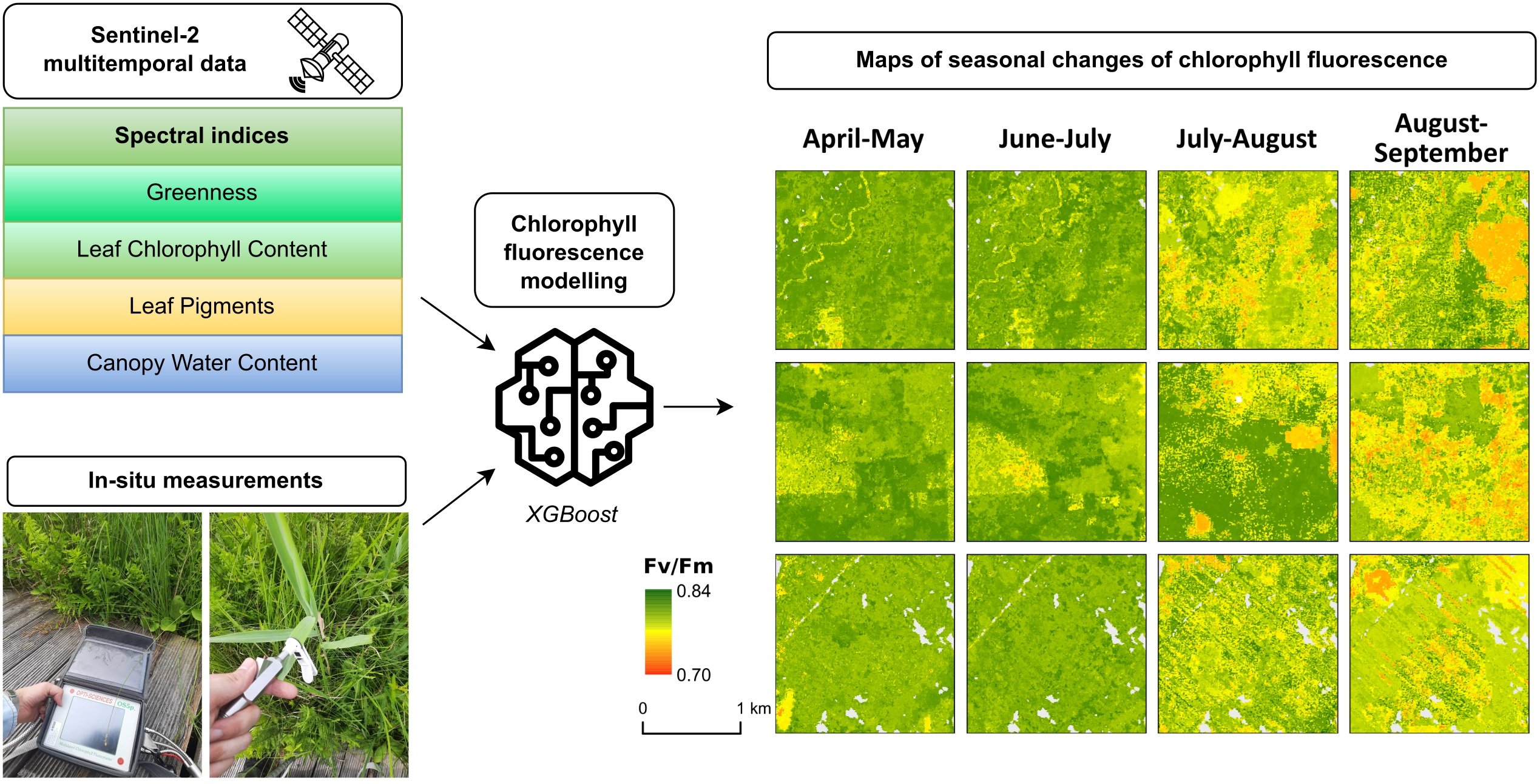
During 2022, five field campaigns were conducted at different times between April and October to collect in situ data, coinciding with Sentinel-2 satellite overpasses around noon local time. Ten sites were selected across various wetland habitats and both sides of the Biebrza River (as shown in Figure 2), and their geographic coordinates were determined using a GNSS receiver. The vegetation’s growth stage was also recorded during each field campaign. The OS5p+ Pulse Modulated Chlorophyll Fluorometer was used to measure ChF in this study [7]. The instrument registers the maximum quantum yield (Fv/Fm) through a dark-adapted test, which is a ratio that represents the maximum potential quantum efficiency of photosystem II (PSII) if all capable reaction centers were open. It estimates the maximum portion of absorbed quanta used in PSII reaction centers [33]. For best results, a dark adaptation time of 20–30 min is recommended [34], and the system provides a series of ten dark-adaption white clips to measure this. After dark adaptation, the end of the fiber optic bundle is placed in the cylindrical opening, and the dark slide of the clip is opened to expose the sample to the fiber optic bundle. Optimal values of Fv/Fm for most land plant species vary within the range of 0.79 to 0.83, while lower values indicate plant stress, particularly photoinhibition [2,8].
2.3. Satellite Data Acquisition
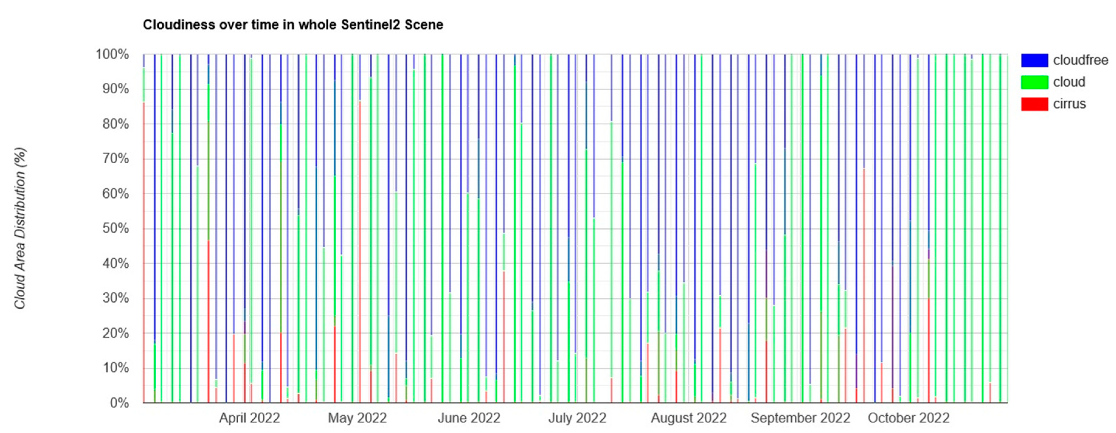
The study area covers two Sentinel-2 granules: 34UFE and 34UEE available from orbits no. 36, 136, and 79 allowing image acquisition every 5–6 days. Satellite images from Sentinel-2A and Sentinel-2B at processing level-2A were retrieved automatically using Google Earth Engine (GEE), i.e., cloud-based platform that provides geospatial data, tools, and computing power for developers to analyze and visualize the world’s satellite imagery and other geospatial data. Users can access and analyze using various programming languages such as Python and JavaScript. It also provides a suite of tools for processing and analyzing the data, including machine learning algorithms for image classification and time-series analysis [35]. For the current study, JavaScript API was used in Earth Engine Code Editor. The average cirrus and cloud cover for the granules in 2022 was 52.15% (Figure 3), whilst the climate in the region is moderate with continental elements, which means that the growing season is short, snow and ice last for a long time, and there is a significant amount of cloud cover. As a result, to create comprehensive images of the area, mosaics were created using images captured by the Sentinel-2 satellite. To combine Sentinel-2 (S-2) data into a mosaic, Google Earth Engine (GEE) uses an algorithm that calculates a high-dimensional weighted geometric median. This approach ensures that the spectral relationships across all the S-2 bands are maintained in the resulting mosaic. Cloudless satellite image mosaics were run spanning around ten days before and after ground measurements. Full list of periods selected for temporal mosaicking of Sentinel-2 images in 2022 over study area is presented in Table 1.
2.4. Vegetation Index Calculation
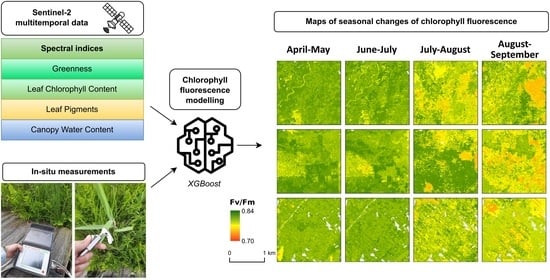
To map the vegetation condition of wetlands using Sentinel-2 data, a total of forty vegetation indices (VIs) were selected and calculated from S2 median mosaics covering the study area. Initially, the most commonly used spectral vegetation indices that describe various aspects of plant growth and health, such as greenness, leaf chlorophyll content, pigments, and water content in the canopy, were identified for the study. These VIs were then arranged into four groups and listed in Table 2.
2.5. Model Establishment and Evaluation
The XGBoost algorithm was investigated to build a model for estimation of chlorophyll fluorescence, which is an open-source software library for gradient boosting algorithms that is designed to be highly efficient, flexible, and scalable. It is a popular machine learning framework that is widely used in industry and academia for supervised learning tasks, such as classification and regression. The XGBoost algorithm works by combining multiple weak models to create a strong model. It trains each model iteratively by adjusting the weights of misclassified samples, with the aim of minimizing a loss function. The final model is a weighted sum of all the models, with the weights determined by their performance on the training data [76]. XGBoost is known for its speed and performance, and it supports regularization, uses the power of parallel processing, handles missing values, and performs cross-validation [77].
The input for the model was an array containing r rows and c columns, where r represents the total number of observations with available data on predictors (vegetation indices) and references (Fv/Fm), and c represents the number of columns with predictors calculated for each growth stage. All the predictors were scaled to a range of values between zero and one. The proposed model in supervised learning referred to the mathematical structure by which the prediction was made from the satellite-based vegetation indices (listed in Table 2). A linear prediction model was created, which calculates predictions based on a combination of weighted satellite-derived data and parameters. The available dataset was split into a training set and a validation set in a ratio of 80:20. To improve the accuracy of the prediction model, the XGBoost algorithm was fine-tuned using tenfold cross-validation and learning curve methods during the training phase to determine the best parameter configuration.
In order to evaluate the performance of the model, a cross-validation was carried out using the leave-one-out approach, which is a variant of k-fold cross-validation, where k is equal to the number of observations in the dataset. It should be noted that the feature selection process was repeated at each iteration to prevent the model from benefiting from knowledge of the data used for validation. The model performance was assessed using various metrics, including the coefficient of determination (R2), which is the square of the correlation coefficient, as well as the mean absolute error (MBE), root mean square error (RMSE), and relative root mean square error (RRMSE).
3. Results
3.1. Analysis of Ground-Measured Chlorophyll Fluorescence
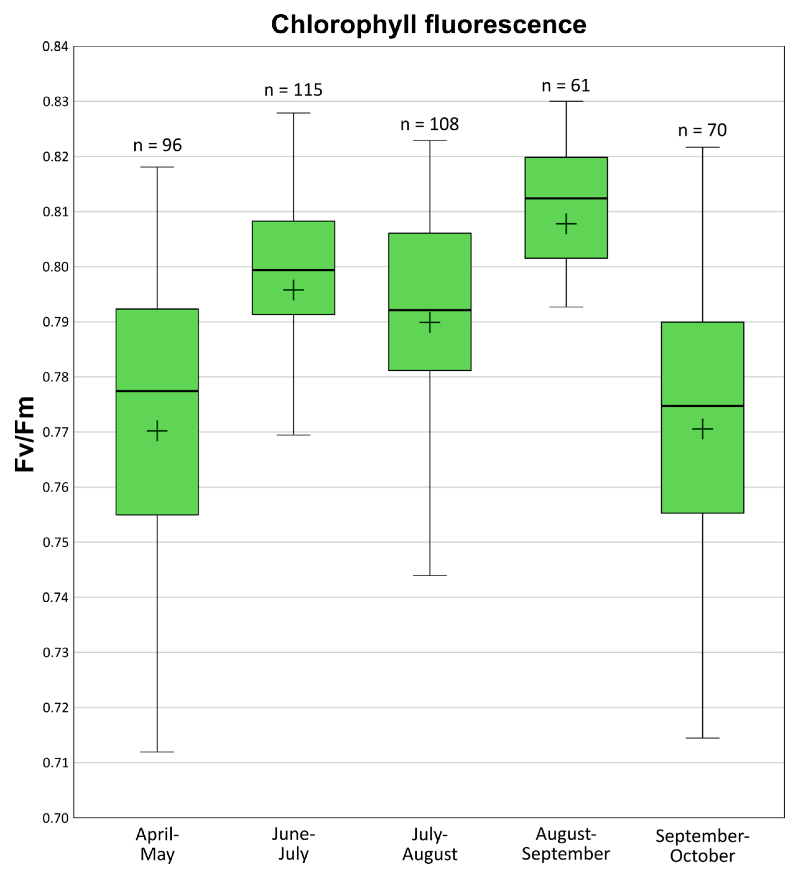
The variations in maximum quantum yield (Fv/Fm) characterizing chlorophyll fluorescence in different vegetation growth periods at the wetlands in 2022 are shown in Figure 4. The most ChF records were made in late June and early July (115), while due to unfavorable weather conditions in the period September–October, only 48 field measurements were carried out. The Fv/Fm reached its maximum value (0.82) at the late flowering stage in August–September. It was noted at its lowest at the late beginning and at the end of the growing season (0.76), in the periods April–May and September–October, respectively. The lowest standard deviations appeared in the mid-season (July–August–September), at 0.010–0.011, whilst the highest standard deviations appeared in the early (April–May) and late stages (September–October) of wetland vegetation development, at 0.026 and 0.029, respectively.
3.2. Features Selected by Algorithm for Mapping ChF
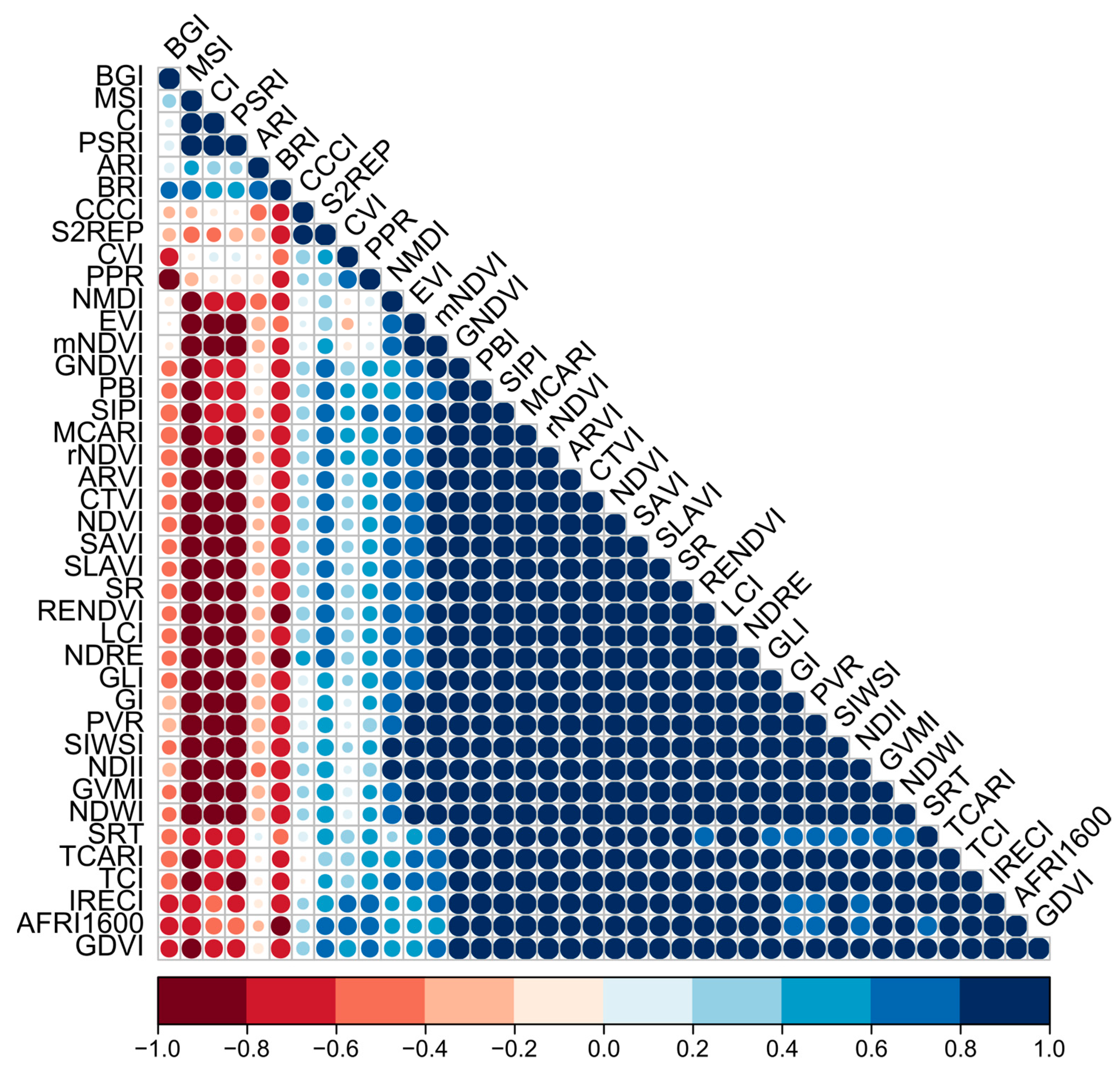
The initial feature set is composed of 19 greenness-related vegetation indices, 7 indices characterizing leaf chlorophyll content, 8 features concerning leaf pigments, and 6 indices on canopy water content. Each feature parameter in the feature set is analyzed individually, and Figure 5 shows the correlation coefficient between each of these parameters. It can be noted that the overall features have high positive and negative correlations with the other ones. The water content, leaf pigments, and canopy structure of herbaceous plants in wetlands exhibit clear changes that can be used to monitor their growth dynamics. Additionally, measuring the chlorophyll content of the canopy is a sensitive method for accurately determining vegetation growth patterns. Among all analyzed features, the indices based on Sentinel-2 spectral bands of near-infrared (NIR) and shortwave-infrared (SWIR) received the most correlations among each other. The parameters related to the water content of the canopy, such as the area and amplitude of the edges in the near-infrared (NIR) and shortwave-infrared (SWIR) regions, exhibit significant changes in response to variations in vegetation conditions caused by river water-level fluctuations and spring floods. The algorithm selects the combination of wavelenghts with the least collinearity, and then the correlation coefficient between each spectral index based on combinations of various wavelengths with another one shows non-uniformity.
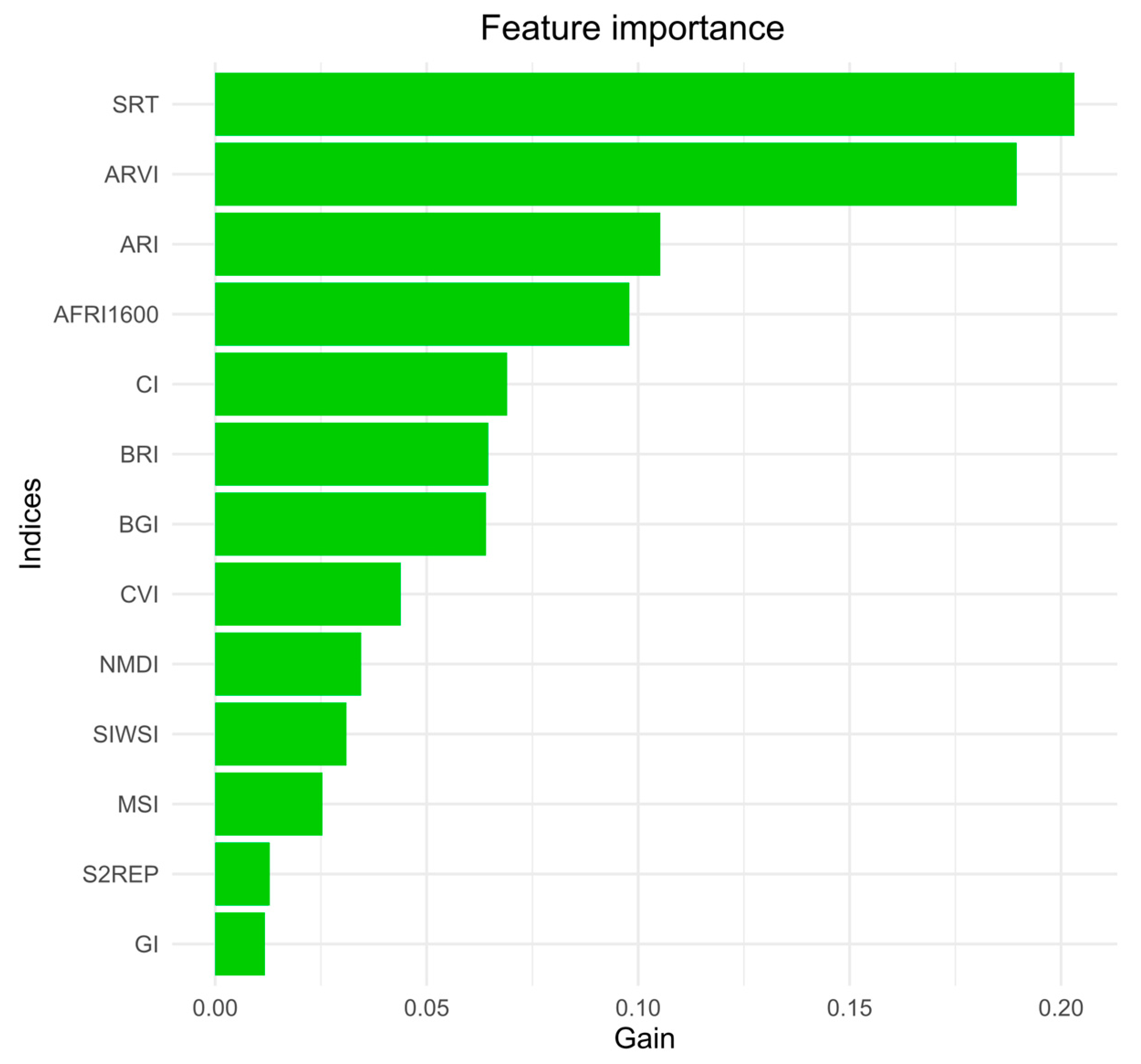
In this study, we examined the use of XGBoost for automating the feature selection process on the initial feature set. The outcome of this process is presented in Figure 6. It can be observed that the Simple Ratio on the 1610 and 2190 bands (SRT) has the highest importance, while the importance of the ARVI is slightly lower. Both indices reflect vegetation growth dynamics and temporal changes in photosynthetic capacity. The vegetation indices ARI, CI, and BRI, which reflect plant senescence, can detect even minor changes in leaf pigments and capture the phenomenon of vegetation browning. When herbaceous plants are exposed to various environmental stresses such as seasonal flooding, high variations in salt levels, low soil oxygen levels, and waves over time, their cell viability and biochemical composition change, which can affect the morphology of leaves, the distribution of leaf inclination, and the structure of the canopy. Therefore, the SRT, which shows healthy and unhealthy vegetation, has a distinct response to environmental conditions. According to a previous study [34], it was found that under saturation conditions, the variation in far-red fluorescence is mainly influenced by the structure of the canopy. The variability in the broadband light spectrum ranging from 641 to 800 nm, which is included in the ARVI and ARI indices, is mainly influenced by the optical properties of leaves and the structural characteristics of the canopy [15]. Finally, these spectral vegetation indices can reflect the vigor of wetland vegetation linked to the changes in leaf and canopy structure and subsequently to chlorophyll fluorescence.
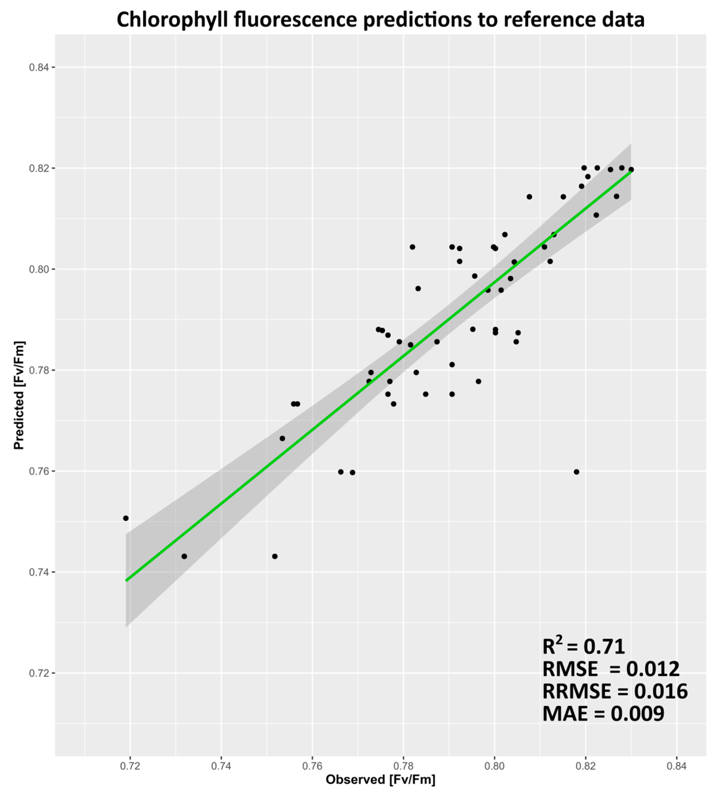
3.3. Evaluation of the Model Performance
To evaluate the XGBoost algorithm results, we compared the predicted chlorophyll fluorescence Fv/Fm with reference data, collected in situ during the growing season in 2022. The evaluation of the model performance is presented in Figure 7. It is worth noting that high coefficients of determination at R2 = 0.71 and low errors at the levels of RMSE = 0.012, rRMSE = 0.016, and MAE = 0.009 were found with the used algorithm. These findings indicate quite good prediction, especially having the short time span of analysis (April–October 2022). The evaluation results indicate that the XGBoost algorithm has high monitoring accuracy, which is consistent with the results of a previous study [78] that used different models. This suggests that the XGBoost algorithm is not only universal but also scalable for vegetation monitoring.
3.4. Spatial and Temporal Patterns of Chlorophyll Fluorescence
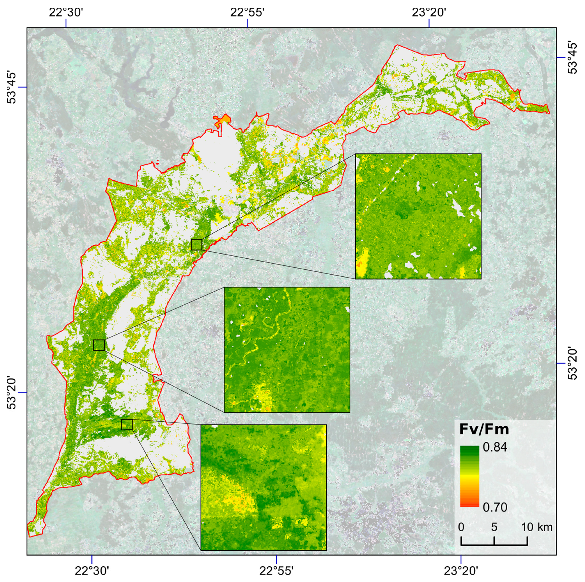
The estimated spatial changes in ChF from April to October 2022 are shown in Figure 8. The areas with non-wetland vegetation such as forests, arables, and meadows were excluded using classification from previous studies [79,80]. Most of the greening areas are in the Biebrza Lower Basin, consistent with the previous studies [26,27,32]. In addition, the spatial estimations on wetland vegetation with high ChF also confirm the results on mapping gross primary productivity (GPP) with remote sensing data from 2022 [80].
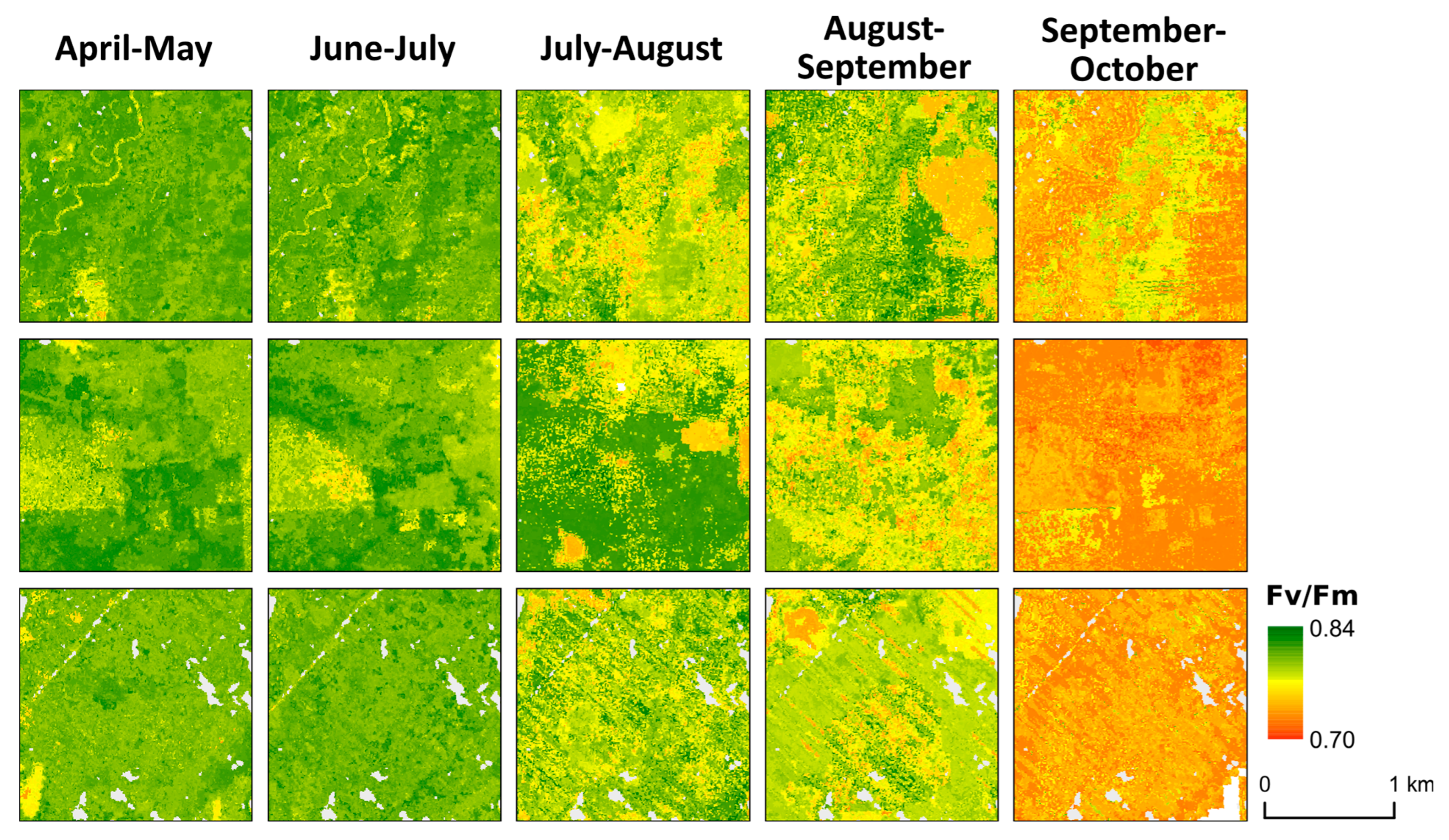
Spatio-temporal changes for five periods are presented in Figure 9. The periods of April–May and June–July exhibit a significant increase in vegetation cover in the Biebrza Valley, particularly in the wild regions of the Biebrza Lower Basin, whilst at the turn of the months July–August, the majority of the Biebrza Valley shows insignificant ChF decreases, with some noticeable browning. This is in agreement with the study of Okruszko, 1990 [29]. During the following month August until October, areas with significant ChF changes were dominated by browning trends under the temperate climate. This is also supported by other studies on Cepkeliai wetlands in Lithuania that are located 200 km from the Biebrza Valley [81]. Moreover, Simanauskiene et al. 2019 [81] found that the summit of the growing season of herbaceous plants is noted in June, while vegetation index variations in July reflect environmental changes indicating browning. The findings suggest that there are significant fluctuations in the spatial distribution of ChF changes across different time periods. We observe an overall greening development stage at a maximum ChF of 0.84 and browning at 0.70.
4. Discussion
The research on a time series of combined optical Sentinel-2 and field remote sensing data led to providing maps of chlorophyll fluorescence over wetlands in a large area. So far, several studies have documented the potential of remote sensing data to map chlorophyll fluorescence [13,16,79]. Whilst Sinha et al. [18] used medium-resolution remote sensing imagery for estimating seasonal fluorescence dynamics at deciduous forests, we mapped the areas difficult to access with high water-level fluctuations. Therefore most studies examined relatively homogeneous areas such as forests; however, larger heterogeneous landscapes with high biodiversity and conservation practices pose a challenge. Nevertheless, the application of Sentinel-2 imagery to estimate chlorophyll fluorescence at wetlands remains underexplored. In this context, we endeavor to figure out the potential of Sentinel-2 multispectral data for estimating the plant state reflecting seasonal variations in phenology at the areas being protected under the Ramsar Convention in Poland. We studied the XGBoost algorithm supported by the combination of Fv/Fm field data to select the most appropriate satellite-derived features for the spatio-temporal monitoring of chlorophyll fluorescence.
Our study demonstrates the potential of 10 m satellite imagery for estimating the chlorophyll fluorescence parameter, which could not be assessed directly from remote sensing data. Comparing coarse-resolution MODIS satellite imagery, Simanauskiene et al. 2019 [81] found that commonly used NDVI values can be recognized as an appropriate indicator for finding degraded peatland areas. However, early detection of degrading peatlands with high spatial and temporal resolution still meets the challenge. Moreover, a suitable algorithm for accurate chlorophyll fluorescence estimation to find the effect of stresses on the photosynthetic process is still required for management practices [82,83,84]. Our study showed a novel approach for mapping ChF and subsequently indicated spatio-temporal greening and browning variations. The features selected by XGBoost enable us to identify plant phenology shifts, such as greening and browning.
Many studies have used the XGBoost algorithm for monitoring environmental changes with remote sensing data [22,23,85]. Jing et al. 2022 [85] found that data collected from one year provide satisfactory results; however, in order to improve the accuracy of prediction on features by XGBoost, more data characterizing meteorological and environmental variables could be included. In our study, spectral vegetation indices and field data were also collected as features with a higher importance in one analyzed year. We are aware that the more field data we collect in subsequent years, the higher accuracy of the model we might assess. The reasons we applied XGBoost are as follows: small dataset (one-year collection), model architecture (decision trees), structured data (Fv/Fm and vegetation indices), and feature importance scores (straightforward and easy to understand). XGBoost and deep learning models are both machine learning algorithms, but they differ in several ways: (a) Model architecture: XGBoost uses an ensemble of decision trees as base learners, whereas deep learning models use artificial neural networks that are composed of multiple layers. (b) Input data format: XGBoost is well-suited for structured data that are arranged in rows and columns, while deep learning models can handle both structured and unstructured data, such as images and text. (c) Computational requirements: deep learning models typically require more computational resources than XGBoost, such as GPUs or TPUs, and can take longer to train. (d) Interpretability: XGBoost provides more interpretability than deep learning models, as it can output feature importance scores and decision rules. In contrast, deep learning models are often considered “black box” models, as it can be difficult to interpret them and understand how they arrive at a particular prediction. (e) Performance on small datasets: XGBoost can perform well on small datasets, whereas deep learning models typically require large amounts of data to perform well.
We utilized Sentinel-2 median mosaics due to cloud coverage frequency at the study site. This process allowed us to reduce the dimensionality of the input array consisting of satellite daily images and adjust the periods of temporal mosaics covering field campaigns at the Biebrza Valley. Results on the quality of the compositions from Sentinel-2 satellite images by Shepherd et al. 2020 [86] confirmed the use of improved cloud-free and composed daily, weekly, or monthly mosaics for regular land monitoring. Regarding unfavorable weather conditions in the study area, Sentinel-2 median mosaics were taken into account as well. In our study, we did not explicitly consider the impact of view zenith angle difference and its derivative consequences on the model performance in temporal pattern prediction [87]. However, this is an important factor to consider in future studies. Therefore, we recommend that future studies investigating temporal patterns in remote sensing data should consider this factor and explicitly evaluate its impact on model performance.
However, some limitations must be mentioned in next future studies. Even though the XGBoost algorithm effectively detected ChF patterns at the local site and the method presented might be applied to other areas, the parameters require further optimization. In this context, the XGBoost model will be developed applying additional parameters characterizing high water-level fluctuations, e.g., surface roughness and soil moisture establishments from satellite radar data. Additionally, regarding weather and optical satellite daily image constraints, the obtained median mosaics were few, and the coverage was limited. Therefore, this study did not focus on large-scale environmental monitoring or detecting stress periods. However, including meteorological information such as air temperature, precipitation, and humidity derived from ERA-5 Land reanalysis could be valuable for future research.
Our study aimed to emphasize the possibility of applying free-of-charge Sentinel-2 imagery for mapping chlorophyll fluorescence with fine resolution. Considering the reports on the state of European wetlands from the EEA and the anthropogenic influence on the wetland biodiversity and sustainable management of the Biebrza Valley in Poland [25,84], the proposed study might support biodiversity conservation and management practices that are the subject of investigations from other academic units [88,89].
5. Conclusions
Our study demonstrates the feasibility of mapping chlorophyll fluorescence for an area of terrestrial wetlands using remote sensing indices derived from the Sentinel-2 satellite with high accuracy (R2 = 0.71, RMSE = 0.012). However, fluorescence information has so far most often been related point-wise to specific study locations. We have shown that by using ground-based field measurements, it is possible to use machine learning techniques (XGBoost algorithm) to relate the solution spatially, enabling the analysis of wetland conditions and wetland phenological changes (growth, full vegetation development, dieback). The conducted feature selection showed that among the most important remote sensing indices in the wetlands were a group of leaf pigment (Anthocyanin Reflectance Index, Coloration Index, Browning Reflectance Index, Blue Green Pigment Index) and water indices (Normalized Multi-band Drought Index, Shortwave Infrared Water Stress Index, Moisture Stress Index). In detail, the group of water indices shows a strong relationship between water content and chlorophyll fluorescence, which demonstrates the high dependence of photosynthesis on water conditions in wetlands, which are an important absorber of atmospheric carbon dioxide, and drainage could adversely affect this potential. Generally, regarding our results and F1 scores presented in Figure 6, the Simple Ratio Index based on Sentinel-2 Short Wave Infrared (B11 and B12) bands revealed the highest importance in the model. AFRI1600 based on Infrared and Short Wave Infrared (Sentinel-2 B8 and B11) is among the crucial features to model as well. However, we are aware that other vegetation indices, such as the ARVI and ARI, which are based on spectral reflections in the visible blue and green bands, also significantly influenced the estimation of chlorophyll fluorescence. Therefore, it is recommended to conduct analyses using a wide range of indices and other biophysical parameters for research purposes. It is important to note that the specific bands used for fluorescence modeling may vary depending on the type of plant or vegetation being studied, as well as the environmental conditions being assessed. This research is a contribution to further fluorescence mapping studies, especially in the context of the upcoming European Space Agency mission, the FLuorescence EXplorer (FLEX), which will aim to determine fluorescence data for the globe on a continuous basis. Further surveys will allow the proposed solution to be extended to other plant ecosystems (forests, agricultural fields), which is particularly important in view of climate change and sustainable agriculture. A possible future direction for the research will be to combine the fluorescence data with other biophysical variables as well as climatic conditions, identifying the relationship between them and their influence on chlorophyll fluorescence.
Author Contributions
Conceptualization, M.B. and M.K.; methodology, M.B. and M.K.; software, M.K.; validation, M.K. and M.B.; formal analysis, M.K. and M.B.; investigation, M.K. and M.B.; resources, M.B.; data curation, M.K. and M.B.; writing—original draft preparation, M.B. and M.K.; writing—review and editing, M.K. and M.B.; visualization, M.K. and M.B.; supervision, M.B.; project administration, M.B.; funding acquisition, M.B. All authors have read and agreed to the published version of the manuscript.
Funding
The field measurements have been funded by the National Science Centre, Poland (NCN), with MINIATURA 5 grant no. 2021/05/X/ST10/00850.
Data Availability Statement
Satellite data are publicly available online: Sentinel-2 images were acquired from the Google Earth Engine (https://earthengine.google.com/; accessed on 1 November 2022). Chlorophyll fluorescence measurements were acquired during field campaigns by all authors, and the data are stored by Maciej Bartold.
Acknowledgments
The authors want to thank the Biebrza National Park for discussions and permission to make the field measurements.
Conflicts of Interest
The authors declare no conflict of interest.
References
- Krause, G.H.; Weis, E. Chlorophyll fluorescence as a tool in plant physiology. Photosynth. Res. 1984, 5, 139–157. [Google Scholar] [CrossRef] [PubMed]
- Maxwell, K.; Johnson, G.N. Chlorophyll fluorescence—A practical guide. J. Exp. Bot. 2000, 51, 659–668. [Google Scholar] [CrossRef] [PubMed]
- Buschmann, C. Variability and application of the chlorophyll fluorescence emission ratio red/far-red of leaves. Photosynth. Res. 2007, 92, 261–271. [Google Scholar] [CrossRef] [PubMed]
- Schreiber, U.; Schliwa, U.; Bilger, W. Continuous recording of photochemical and non-photochemical chlorophyll fluorescence quenching with a new type of modulation fluorometer. Photosynth. Res. 1986, 10, 51–62. [Google Scholar] [CrossRef]
- Michele, M.; Micol, R.; Luis, G.; Luis, A.; Roberto, C.; Jose, M. Remote sensing of solar-induced chlorophyll fluorescence: Review of methods and applications. Remote Sens. Environ. 2009, 113, 2037–2051. [Google Scholar] [CrossRef]
- Mohammed, G.H.; Colombo, R.; Middleton, E.M.; Rascher, U.; van der Tol, C.; Nedbal, L.; Goulas, Y.; Pérez-Priego, O.; Damm, A.; Meroni, M.; et al. Remote sensing of solar-induced chlorophyll fluorescence (SIF) in vegetation: 50 years of progress. Remote Sens. Environ. 2019, 231, 111177. [Google Scholar] [CrossRef]
- OS5p+ Pulse Modulated Chlorophyll Fluorometer, User Guide, OptiScience. 2022. Available online: https://www.optisci.com/ (accessed on 1 April 2023).
- Baker, N.R.; Oxborough, K. Chlorophyll Fluorescence as a Probe of Photosynthetic Productivity. In Chlorophyll a Fluorescence. Advances in Photosynthesis and Respiration; Papageorgiou, G.C., Govindjee, Eds.; Springer: Dordrecht, The Netherlands, 2004; Volume 19. [Google Scholar] [CrossRef]
- Du, S.; Liu, L.; Liu, X.; Hu, J. Response of Canopy Solar-Induced Chlorophyll Fluorescence to the Absorbed Photosynthetically Active Radiation Absorbed by Chlorophyll. Remote Sens. 2017, 9, 911. [Google Scholar] [CrossRef]
- Jia, M.; Li, D.; Colombo, R.; Wang, Y.; Wang, X.; Cheng, T.; Zhu, Y.; Yao, X.; Xu, C.; Ouer, G.; et al. Quantifying Chlorophyll Fluorescence Parameters from Hyperspectral Reflectance at the Leaf Scale under Various Nitrogen Treatment Regimes in Winter Wheat. Remote Sens. 2019, 11, 2838. [Google Scholar] [CrossRef]
- Joiner, J.; Guanter, L.; Lindstrot, R.; Voigt, M.; Vasilkov, A.; Middleton, E.; Huemmrich, K.; Yoshida, Y.; Frankenberg, C. Global monitoring of terrestrial chlorophyll fluorescence from moderate-spectral-resolution near-infrared satellite measurements: Methodology, simulations, and application to GOME-2. Atmos. Meas. Tech. 2013, 6, 3883–3930. [Google Scholar] [CrossRef]
- Duveiller, G.; Filipponi, F.; Walther, S.; Köhler, P.; Frankenberg, C.; Guanter, L.; Cescatti, A. A spatially downscaled sun-induced fluorescence global product for enhanced monitoring of vegetation productivity. Earth Syst. Sci. Data 2020, 12, 1101–1116. [Google Scholar] [CrossRef]
- Li, X.; Xiao, J.; He, B.; Arain, M.A.; Beringer, J.; Desai, A.R.; Emmel, C.; Hollinger, D.Y.; Krasnova, A.; Mammarella, I.; et al. Solar-induced chlorophyll fluorescence is strongly correlated with terrestrial photosynthesis for a wide variety of biomes: First global analysis based on OCO-2 and flux tower observations. Glob. Change Biol. 2018, 24, 3990–4008. [Google Scholar] [CrossRef] [PubMed]
- Campbell, P.K.E.; Huemmrich, K.F.; Middleton, E.M.; Ward, L.A.; Julitta, T.; Daughtry, C.S.T.; Burkart, A.; Russ, A.L.; Kustas, W.P. Diurnal and Seasonal Variations in Chlorophyll Fluorescence Associated with Photosynthesis at Leaf and Canopy Scales. Remote Sens. 2019, 11, 488. [Google Scholar] [CrossRef]
- Radosław, G.; Maciej, B. Remote sensing techniques to assess chlorophyll fluorescence in support of crop monitoring in Poland. Misc. Geogr. 2021, 25, 226–237. [Google Scholar] [CrossRef]
- Guo, M.; Li, J.; Li, J.; Zhong, C.; Zhou, F. Solar-Induced Chlorophyll Fluorescence Trends and Mechanisms in Different Ecosystems in Northeastern China. Remote Sens. 2022, 14, 1329. [Google Scholar] [CrossRef]
- Kritten, L.; Preusker, R.; Fischer, J. A New Retrieval of Sun-Induced Chlorophyll Fluorescence in Water from Ocean Colour Measurements Applied on OLCI L-1b and L-2. Remote Sens. 2020, 12, 3949. [Google Scholar] [CrossRef]
- Sinha, S.K.; Padalia, H.; Patel, N.R.; Chauhan, P. Estimation of Seasonal Sun-Induced Fluorescence Dynamics of Indian Tropical Deciduous Forests using SCOPE and Sentinel-2 MSI. Int. J. Appl. Earth Obs. Geoinf. 2020, 91, 102155. [Google Scholar] [CrossRef]
- Buman, B.; Hueni, A.; Colombo, R.; Cogliati, S.; Celesti, M.; Julitta, T.; Burkart, A.; Siegmann, B.; Rascher, U.; Drusch, M.; et al. Towards consistent assessments of in situ radiometric measurements for the validation of fluorescence satellite missions. Remote Sens. Environ. 2022, 274, 112984. [Google Scholar] [CrossRef]
- Poddar, S.; Chacko, N.; Swain, D. Estimation of Chlorophyll-a in Northern Coastal Bay of Bengal Using Landsat-8 OLI and Sentinel-2 MSI Sensors. Front. Mar. Sci. 2019, 6, 598. [Google Scholar] [CrossRef]
- Smith, B.; Pahlevan, N.; Schalles, J.; Ruberg, S.; Errera, R.; Ma, R.; Giardino, C.; Bresciani, M.; Barbosa, C.; Moore, T.; et al. A Chlorophyll-a Algorithm for Landsat-8 Based on Mixture Density Networks. Front. Remote Sens. 2021, 1, 623678. [Google Scholar] [CrossRef]
- Young, K.; Taeho, K.; Jihoon, S.; Dae-Seong, L.; Park, Y.-S.; Yeji, K.; Yoonkyung, C. Validity evaluation of a machine-learning model for chlorophyll a retrieval using Sentinel-2 from inland and coastal waters. Ecol. Indic. 2022, 137, 108737. [Google Scholar] [CrossRef]
- Shi, X.; Gu, L.; Jiang, T.; Zheng, X.; Dong, W.; Tao, Z. Retrieval of Chlorophyll-a Concentrations Using Sentinel-2 MSI Imagery in Lake Chagan Based on Assessments with Machine Learning Models. Remote Sens. 2022, 14, 4924. [Google Scholar] [CrossRef]
- Wassen, M.; Okruszko, T.; Kardel, I.; Chormański, J.; Świątek, D.; Mioduszewski, W.; Bleuten, W.; Querner, E.; El Kahloun, M.; Batellan, O.; et al. Eco-Hydrological Functioning of Biebrza Wetlands: Lessons for the Conservation and Restoration of Deteriorated Wetlands. Ecol. Stud. 2006, 191, 285–310. [Google Scholar]
- Ignacy, K.; Dorota, S.; Jaroslaw, C.; Tomasz, O.; Martin, W. Water management decision support system for biebrza national park. Environ. Prot. Eng. 2009, 35, 173–180. [Google Scholar]
- Budzyńska, M.; Dąbrowska-Zielińska, K.; Turlej, K.; Małek, I.; Bartold, M. Monitoring of the Biebrza Wetlands using remote sensing methods. Water-Environ.-Rural. Areas 2011, 11, 39–64. [Google Scholar]
- Dabrowska-Zielinska, K.; Budzynska, M.; Tomaszewska, M.; Bartold, M.; Gatkowska, M.; Malek, I.; Turlej, K.; Napiorkowska, M. Monitoring Wetlands Ecosystems Using ALOS PALSAR (L-Band, HV) Supplemented by Optical Data: A Case Study of Biebrza Wetlands in Northeast Poland. Remote Sens. 2014, 6, 1605–1633. [Google Scholar] [CrossRef]
- Dabrowska-Zielinska, K.; Budzynska, M.; Tomaszewska, M.; Malinska, A.; Gatkowska, M.; Bartold, M.; Malek, I. Assessment of Carbon Flux and Soil Moisture in Wetlands Applying Sentinel-1 Data. Remote Sens. 2016, 8, 756. [Google Scholar] [CrossRef]
- Okruszko, H. Wetlands of the Biebrza valley, Their Value and Future Management; Polish Academy of Sciences: Warsaw, Poland, 1990. [Google Scholar]
- Pawłowski, B.; Medwecka-Kornaś, A.; Kornaś, J. Review of Terrestrial and Fresh-water Plant Communities. In International Series of Monographs in Pure and Applied Biology; The Vegetation of Poland; Szafer, W., Ed.; Wiley-Blackwell Publishing Ltd.: Hoboken, NJ, USA, 1966; Volume 9. [Google Scholar] [CrossRef]
- Okruszko, T.; Chormański, J.; Mirosław-Świątek, D.; Gregorczyk, M. Hydrological Characteristics of Swamp Communities, the Biebrza River (NE Poland) Case Study; Environmental Hydraulics Taylor & Francis Group: London, UK, 2010; pp. 407–412. [Google Scholar]
- Tomasz, B.; Martin, W.; Jan, S.; Jaroslaw, C.; Stefan, I.; Okke, B.; Tomasz, O. Wetlands in flux: Looking for the drivers in a central European case. Wetl. Ecol. Manag. 2018, 26, 849–863. [Google Scholar] [CrossRef]
- Kitajima, M.; Butler, W.L. Quenching of chlorophyll fluorescence and primary photochemistry in chloroplasts by dibromothymoquinone. Biochim. Biophys. Acta 1975, 376, 105–115. [Google Scholar] [CrossRef] [PubMed]
- Kycko, M.; Romanowska, E.; Zagajewski, B. Lead-Induced Changes in Fluorescence and Spectral Characteristics of Pea Leaves. Remote Sens. 2019, 11, 1885. [Google Scholar] [CrossRef]
- Gorelick, N.; Hancher, M.; Dixon, M.; Ilyushchenko, S.; Thau, D.; Moore, R. Google Earth Engine: Planetary-scale geospatial analysis for everyone. Remote Sens. Environ. 2017, 202, 18–27. [Google Scholar] [CrossRef]
- Available online: https://philippgaertner.github.io/2020/08/percent-cloud-cover/ (accessed on 28 February 2023).
- Arnon, K.; Yoram, K.; Lorraine, R.; Andrew, W. AFRI—Aerosol free vegetation index. Remote Sens. Environ. 2001, 71, 10–21. [Google Scholar]
- Kaufman, Y.J.; Tanré, D. Atmospherically Resistant Vegetation Index (ARVI) for EOS-MODIS. IEEE Trans. Geosci. Remote Sens. 1992, 30, 261–270. [Google Scholar] [CrossRef]
- Perry, C., Jr.; Lautenschlager, L.F. Functional Equivalence of Spectral Vegetation Indices. Remote Sens. Environ. 1984, 14, 169–182. [Google Scholar] [CrossRef]
- Huete, A.R.; Justice, C.; Liu, H. Development of vegetation soil indices for, M.O.D.I.S.-E.O.S. Remote Sens. Environ. 1994, 49, 224–234. [Google Scholar] [CrossRef]
- Sripada, R.P.; Heiniger, R.W.; White, J.G.; Weisz, R. Aerial color infrared photography for determining late-season nitrogen requirements in corn. Agron. J. 2005, 97, 1443–1451. [Google Scholar] [CrossRef]
- Li, Y.; Chen, D.; Walker, C.N.; Angus, J.F. Estimating The Nitrogen Status Of Crops Using A Digital Camera. Field Crops Res. 2010, 118, 221–227. [Google Scholar] [CrossRef]
- Gitelson, A.; Merzlyak, M.N. Quantitative estimation of chlorophyll a using reflectance spectra: Experiments with autumn chestnut and maple leaves. J. Photochem. Photobiol. B Biol. 1994, 22, 247–252. [Google Scholar] [CrossRef]
- Jurgens, C. The modified normalized difference vegetation index (mNDVI) a new index to determine frost damages in agriculture based on Landsat TM data. Int. J. Remote Sens. 1997, 18, 3583–3594. [Google Scholar] [CrossRef]
- Rouse, J.W.; Haas, R.H.; Schell, J.A.; Deering, D.W. Monitoring Vegetation Systems in the Great Plains with E.R.T.S. In Proceedings of the 3rd Earth Resources Technology Satellite Symposium, Washington, DC, USA, 10–14 December 1973; pp. 309–317. [Google Scholar]
- Roujean, J.; Breon, F. Estimating PAR Absorbed by Vegetation from Bidirectional Reflectance Measurements. Remote Sens. Environ. 1995, 51, 375–384. [Google Scholar] [CrossRef]
- Edward, B.; Clarke, T.R.; Richards, S.E.; Paul, C.; Julio, H.; Kostrzewski, M.; Peter, W.; Christopher, C.; Riley, E.; Thompson, T.L. Coincident detection of crop water stress, nitrogen status, and canopy density using ground based multispectral data. In Proceedings of the the Fifth International Conference on Precision Agriculture, Bloomington, MN, USA, 16–19 July 2000. [Google Scholar]
- Graciela, M. Vegetation indices derived from high-resolution airborne videography for precision crop management. Int. J. Remote Sens. 2003, 24, 2855–2877. [Google Scholar] [CrossRef]
- Gitelson, A.; Merzlyak, M. Spectral Reflectance Changes Associated with Autumn Senescence of Aesculus Hippocastanum L. and Acer platanoides L. Leaves. J. Plant. Physiol. 1994, 143, 286–292. [Google Scholar] [CrossRef]
- Sims, D.; Gamon, J. Relationships Between Leaf Pigment Content and Spectral Reflectance Across a Wide Range of Species, Leaf Structures and Developmental Stages. Remote Sens. Environ. 2002, 81, 337–354. [Google Scholar] [CrossRef]
- Huete, A.R. A soil adjusted vegetation index SAVI. Remote Sens. Environ. 1988, 25, 295–309. [Google Scholar] [CrossRef]
- LLymburner, P.J.; Beggs, C.R. Jacobson, Estimation of canopy-average surface-specific leaf area using Landsat TM data. Photogramm. Eng. Remote Sens. 2000, 66, 183–191. [Google Scholar]
- Jordan, C.F. Derivation of leaf area index from quality of light on the forest floor. Ecology 1969, 50, 663–666. [Google Scholar] [CrossRef]
- Pearson, R.L.; Miller, L.D. Remote mapping of standing crop biomass for estimation of the productivity of the shortgrass prairie. In Proceedings of the Eighth International Symposium on Remote Sensing of Environment, Ann Arbor, MI, USA, 2–6 October 1972; Environmental Research Institute of Michigan: Ann Arbor, MI, USA, 1972; pp. 1357–1381. [Google Scholar]
- Frederic, B.; Guyot, G.; Bégué, A.; Maurel, P.; Podaire, A. Complementarity of middle-infrared with visible and near-infrared reflectance for monitoring wheat canopies. Remote Sens. Environ. 1988, 26, 213–225. [Google Scholar] [CrossRef]
- Frampton, W.; Dash, J.; Watmough, G.; Milton, E. Evaluating the capabilities of Sentinel-2 for quantitative estimation of biophysical variables in vegetation. ISPRS J. Photogramm. Remote Sens. 2013, 82, 83–92. [Google Scholar] [CrossRef]
- Elshikha, D.E.; Barnes, E.; Clarke, T.; Hunsaker, D.; Haberland, J.; Pinter, P.; Waller, P.; Thompson, T.L. Remote Sensing of Cotton Nitrogen Status Using the Canopy Chlorophyll Content Index (CCCI). Trans. ASABE 2008, 51, 73–82. [Google Scholar] [CrossRef]
- Gitelson, A.A.; Gritz, Y.; Merzlyak, M.N. Relationships between leaf chlorophyll content and spectral reflectance and algorithms for non-destructive chlorophyll assessment in higher plant leaves. J. Plant. Physiol. 2003, 160, 271–282. [Google Scholar] [CrossRef]
- Datt, B. Remote Sensing of Water Content in Eucalyptus Leaves. J. Plant. Physiol. 1999, 154, 30–36. [Google Scholar] [CrossRef]
- Daughtry, C.S.T.; Walthall, C.L.; Kim, M.S.; Brown de Colstoun, E.; McMurtrey, J.E. Estimating corn leaf chlorophyll concentration for leaf and canopy reflectance. Remote Sens. Environ. 2000, 74, 229–239. [Google Scholar] [CrossRef]
- Haboudane, D.; Miller, J.R.; Tremblay, N.; Zarco-Tejada, P.J.; Dextraze, L. Integrated narrow-band vegetation indices for prediction of crop chlorophyll content for application to precision agriculture. Remote Sens. Environ. 2002, 81, 416–426. [Google Scholar] [CrossRef]
- Haboudane, D.; Tremblay, N.; Miller, J.R.; Vigneault, P. Remote estimation of crop chlorophyll content using spectral indices derived from hyperspectral data. IEEE Trans. Geosci. Remote Sens. 2008, 46, 423–437. [Google Scholar] [CrossRef]
- Gitelson, A.; Merzlyak, M.; Chivkunova, O. Optical Properties and Nondestructive Estimation of Anthocyanin Content in Plant Leaves. Photochem. Photobiol. 2001, 71, 38–45. [Google Scholar] [CrossRef]
- Zarco-Tejada, P.J.; Berjón, A.; López-Lozano, R.; Miller, J.R.; Matín, P.; Cachorro, V.; Gonzáles, M.R.; de Frutos, A. Assessing vineyard condition with hyperspectral indices: Leaf and canopy reflectance simulation in a row structured discontinuous canopy. Remote Sens. Environ. 2005, 99, 271–287. [Google Scholar] [CrossRef]
- Chivkunova, O.; Solovchenko, A.; Sokolova, S.; Merzlyak, M.; Reshetnikova, I. Reflectance Spectral Features and Detection of Superficial Scald–induced Browning in Storing Apple Fruit. Pap. Nat. Resour. 2001, 2, 267. [Google Scholar]
- Louhaichi, M.; Borman, M.M.; Johnson, D.E. Spatially located platform and aerial photography for documentation of grazing impacts on wheat. Geocarto Int. 2001, 16, 65–70. [Google Scholar] [CrossRef]
- Nidamanuri, R.; Garg, P.K.; Sanjay, G.; Vinay, D. Estimation of leaf total chlorophyll and nitrogen concentrations using hyperspectral satellite imagery. J. Agric. Sci. 2008, 146, 65–75. [Google Scholar]
- Merzlyak, M.N.; Gitelson, A.A.; Chivkunova, O.B.; Rakitin, V.Y. Non-destructive optical detection of pigment changes during leaf senescence and fruit ripening. Physiol. Plant. 1999, 106, 135–141. [Google Scholar] [CrossRef]
- Josep, P.; Baret, F.; Iolanda, F. Semi-Empirical Indices to Assess Carotenoids/Chlorophyll—A Ratio from Leaf Spectral Reflectance. Photosynthetica 1995, 31, 221–230. [Google Scholar]
- Ceccato, P.; Gobron, N.; Flasse, S.; Pinty, B.; Tarantola, S. Designing a spectral index to estimate vegetation water content from remote sensing data: Part 1 Theoretical approach. Remote Sens. Environ. 2002, 82, 188–197. [Google Scholar] [CrossRef]
- Hunt, E.R.; Rock, B.N. Detection of changes in leaf water content using near- and middle-infrared reflectances. Remote Sens. Environ. 1989, 30, 43–54. [Google Scholar]
- Hardisky, M.A.; Klemas, V.; Smart, R.M. The influence of soil salinity, growth form, and leaf moisture on the spectral reflectances of Spartina alterniflora canopies. Photogramm. Eng. Remote Sens. 1983, 49, 77–83. [Google Scholar]
- Gao, B. NDWI—A normalized difference water index for remote sensing of vegetation liquid water from space. Remote Sens. Environ. 1996, 58, 257–266. [Google Scholar] [CrossRef]
- Wang, L.; Qu, J.J. NMDI: A normalized multi-band drought index for monitoring soil and vegetation moisture with satellite remote sensing. Geophys. Res. Lett. 2007, 34, L20405. [Google Scholar] [CrossRef]
- Rasmus, F.; Inge, S. Derivation of a Shortwave Infrared Water Stress Index From MODIS Near- and Shortwave Infrared Data in a Semiarid Environment. Remote Sens. Environ. 2003, 87, 111–121. [Google Scholar]
- Wen, L.; Hughes, M. Coastal Wetland Mapping Using Ensemble Learning Algorithms: A Comparative Study of Bagging, Boosting and Stacking Techniques. Remote Sens. 2020, 12, 1683. [Google Scholar] [CrossRef]
- Jafarzadeh, H.; Mahdianpari, M.; Gill, E.W.; Brisco, B.; Mohammadimanesh, F. Remote Sensing and Machine Learning Tools to Support Wetland Monitoring: A Meta-Analysis of Three Decades of Research. Remote Sens. 2022, 14, 6104. [Google Scholar] [CrossRef]
- Sun, Y.; Liu, T.; Wang, X.; Hu, Y. Chlorophyll Fluorescence Imaging Combined with Active Oxygen Metabolism for Classification of Similar Diseases in Cucumber Plants. Agronomy 2023, 13, 700. [Google Scholar] [CrossRef]
- Dąbrowska-Zielińska, K.; Misiura, K.; Malińska, A.; Gurdak, R.; Bartold, M.; Kluczek, M.; Grzybowski, P. Modelling Net Ecosystem Exchange in the Biebrza Wetlands using satellite and meteorological data. Misc. Geogr. 2022, 26, 215–226. [Google Scholar] [CrossRef]
- Dąbrowska-Zielińska, K.; Misiura, K.; Malińska, A.; Gurdak, R.; Grzybowski, P.; Bartold, M.; Kluczek, M. Spatiotemporal estimation of gross primary production for terrestrial wetlands using satellite and field data. Remote Sens. Appl. Soc. Environ. 2022, 27, 100786. [Google Scholar] [CrossRef]
- Šimanauskienė, R.; Linkevičienė, R.; Bartold, M.; Dąbrowska-Zielińska, K.; Slavinskienė, G.; Veteikis, D.; Taminskas, J. Peatland degradation: The relationship between raised bog hydrology and normalized difference vegetation index. Ecohydrology 2019, 12, e2159. [Google Scholar] [CrossRef]
- Amoros-Lopez, J.; Vila-Frances, J.; Gomez-Chova, L.; Alonso, L.; Guanter, L.; del Valle-Tascon, S.; Calpe, J.; Moreno, J. Remote sensing of chlorophyll fluorescence for estimation of stress in vegetation. recommendations for future missions. In Proceedings of the 2007 IEEE International Geoscience and Remote Sensing Symposium, Barcelona, Spain, 23–28 July 2007; pp. 3769–3772. [Google Scholar] [CrossRef]
- Batelaan, O.; Okruszko, T.; Mirosław-Świątek, D.; Sylwia, S.-W.; Jaroslaw, C.; Martin, W.; Van Loon, A.; Penning, W. Biebrza wetland research: Required science for sustainable management. In Proceedings of the 15th Annual Sustainable Development Research Conference, Utrecht, The Netherlands, 5–8 July 2009. [Google Scholar]
- Sucholas, J.; Molnár, Z.; Łuczaj, Ł.; Poschlod, P. Local traditional ecological knowledge about hay management practices in wetlands of the Biebrza Valley, Poland. J. Ethnobiol. Ethnomedicine 2022, 18, 9. [Google Scholar] [CrossRef]
- Jing, X.; Zou, Q.; Yan, J.; Dong, Y.; Li, B. Remote Sensing Monitoring of Winter Wheat Stripe Rust Based on mRMR-XGBoost Algorithm. Remote Sens. 2022, 14, 756. [Google Scholar] [CrossRef]
- Shepherd, J.D.; Schindler, J.; Dymond, J.R. Automated Mosaicking of Sentinel-2 Satellite Imagery. Remote Sens. 2020, 12, 3680. [Google Scholar] [CrossRef]
- Cui, Z.; Kerekes, J.P. Impact of Wavelength Shift in Relative Spectral Response at High Angles of Incidence in Landsat-8 Operational Land Imager and Future Landsat Design Concepts. IEEE Trans. Geosci. Remote Sens. 2018, 56, 5873–5883. [Google Scholar] [CrossRef]
- Swiatek, D.; Szporak-Nasilowska, S.; Chormanski, J.; Okruszko, T. Hydrodynamic model of the Lower Biebrza River flow—A tool for assessing the hydrologic vulnerability of a floodplain to management practices. Ecohydrol. Hydrobiol. 2008, 8, 331–337. [Google Scholar]
- Grygoruk, M.; Okruszko, T. Do Water Management and Climate-Adapted Management of Wetlands Interfere in Practice? Lessons from the Biebrza Valley, Poland. In Wetlands and Water Framework Directive. GeoPlanet: Earth and Planetary Sciences; Ignar, S., Grygoruk, M., Eds.; Springer: Cham, Switzerland, 2015. [Google Scholar] [CrossRef]
Figure 1.
Major types of wetland vegetation with predominance of sedges (left), sedge mosses (middle), and reeds (right). Photo credit: Marcin Kluczek.
Figure 1.
Major types of wetland vegetation with predominance of sedges (left), sedge mosses (middle), and reeds (right). Photo credit: Marcin Kluczek.

Figure 2.
Locations of field measurements conducted within Biebrza National Park highlighted by red dots and presented on Sentinel-2 median mosaic comprising cloudless satellite images from June–July 2022.
Figure 2.
Locations of field measurements conducted within Biebrza National Park highlighted by red dots and presented on Sentinel-2 median mosaic comprising cloudless satellite images from June–July 2022.

Figure 3.
Cloud area distribution during growing season in 2022 at Sentinel-2 scenes covering Biebrza Wetlands study area (source code: [36]).
Figure 3.
Cloud area distribution during growing season in 2022 at Sentinel-2 scenes covering Biebrza Wetlands study area (source code: [36]).

Figure 4.
Boxplots of maximum quantum yield (Fv/Fm) in the growing season at wetlands in 2022. The box plot shows the median value (line dividing the box plot), the 25th to 75th percentile range (green rectangle), and the mean value (represented by a black cross) of the field measurements (n).
Figure 4.
Boxplots of maximum quantum yield (Fv/Fm) in the growing season at wetlands in 2022. The box plot shows the median value (line dividing the box plot), the 25th to 75th percentile range (green rectangle), and the mean value (represented by a black cross) of the field measurements (n).

Figure 5.
Correlation coefficient of each Sentinel-2 satellite-derived vegetation index.

Figure 6.
Ranking of features calculated by XGBoost by gain parameter.

Figure 7.
Chlorophyll fluorescence predictions from XGBoost algorithm on validation dataset (abbreviations: RMSE—Root Mean Square Error, RRMSE—Relative Root Mean Square Error, MBE—Mean Absolute Error).
Figure 7.
Chlorophyll fluorescence predictions from XGBoost algorithm on validation dataset (abbreviations: RMSE—Root Mean Square Error, RRMSE—Relative Root Mean Square Error, MBE—Mean Absolute Error).

Figure 8.
Spatial estimation of chlorophyll fluorescence based on Sentinel-2 June–July mosaic. Areas of interest mapped applying wetland vegetation classification elaborated in previous studies [79,80].

Figure 9.
Overview of the predicted chlorophyll fluorescence expressed by Fv/Fm values during the growing season in 2022.
Figure 9.
Overview of the predicted chlorophyll fluorescence expressed by Fv/Fm values during the growing season in 2022.


Table 1.
Sentinel-2 imaging periods used for generating cloudless median mosaics.
| Name | Start Date | End Date | No. of Sentinel-2 Acquisition Dates Used for Mosaic |
|---|---|---|---|
| April–May | 25 April 2022 | 12 May 2022 | 7 |
| June–July | 20 June 2022 | 7 July 2022 | 9 |
| July–August | 20 July 2022 | 4 August 2022 | 7 |
| August–September | 20 August 2022 | 8 September 2022 | 10 |
| September–October | 20 September 2022 | 28 October 2022 | 14 |
Table 2.
List of spectral-vegetation-index-dedicated Sentinel-2 bands used for the study.
| Application | Abbreviation | Name | Equation | Citation |
|---|---|---|---|---|
| Spectral Indices of Greenness | AFRI1600 | Aerosol Free Vegetation Index 1600 | [37] | |
| ARVI | Atmospherically Resistant Vegetation Index | [38] | ||
| CTVI | Corrected Transformed Vegetation Index | [39] | ||
| EVI | Enhanced Vegetation Index | [40] | ||
| GDVI | Green Difference Vegetation Index | [41] | ||
| GI | Greenness Index | [42] | ||
| GNDVI | Green Normalized Difference Vegetation Index | [43] | ||
| mNDVI | Modified NDVI | [44] | ||
| NDVI | Normalized Difference Vegetation Index | [45] | ||
| rNDVI | Renormalized Difference Vegetation Index | [46] | ||
| NDRE | Normalized Difference NIR / Red Edge | [47] | ||
| PPR | Normalized Difference 550/450 Plant Pigment Ratio | [48] | ||
| PVR | Normalized Difference 550/650 Photosynthetic Vigour Ratio | [48] | ||
| RENDVI | Red Edge Normalized Difference Vegetation Index | [49,50] | ||
| SAVI | Soil Adjusted Vegetation Index | [51] | ||
| SLAVI | Specific Leaf Area Vegetation Index | [52] | ||
| SR | Simple Ratio 842/665 | [53,54] | ||
| SRT | Simple Ratio 1610/2190 | [55] | ||
| S2REP | Sentinel-2 Red-Edge Position Index | [56] | ||
| Leaf Chlorophyll Content | CCCI | Canopy Chlorophyll Content Index | [57] | |
| CVI | Red-edge-band Chlorophyll Index | [58] | ||
| IRECI | Inverted Red-edge Chlorophyll Index | [56] | ||
| LCI | Leaf Chlorophyll Index | [59] | ||
| MCARI | Modified Chlorophyll Absorption in Reflectance Index | [60] | ||
| TCARI | Transformed Chlorophyll Absorption Ratio | [61] | ||
| TCI | Triangular Chlorophyll Index | [62] | ||
| Leaf Pigments | ARI | Anthocyanin Reflectance Index | [63] | |
| BGI | Blue Green Pigment Index | [64] | ||
| BRI | Browning Reflectance Index | [65] | ||
| CI | Coloration Index | [58] | ||
| GLI | Green Leaf Index | [66] | ||
| PBI | Plant Biochemical Index | [67] | ||
| PSRI | Plant Senescence Reflectance Index | [68] | ||
| SIPI | Structure Insensitive Pigment Index | [69] | ||
| Canopy Water Content | GVMI | Global Vegetation Moisture Index | [70] | |
| MSI | Moisture Stress Index | [71] | ||
| NDII | Normalized Difference Infrared Index | [72] | ||
| NDWI | Normalized Difference Water Index | [73] | ||
| NMDI | Normalized Multi-band Drought Index | [74] | ||
| SIWSI | Shortwave Infrared Water Stress Index | [75] |
Disclaimer/Publisher’s Note: The statements, opinions and data contained in all publications are solely those of the individual author(s) and contributor(s) and not of MDPI and/or the editor(s). MDPI and/or the editor(s) disclaim responsibility for any injury to people or property resulting from any ideas, methods, instructions or products referred to in the content. |
© 2023 by the authors. Licensee MDPI, Basel, Switzerland. This article is an open access article distributed under the terms and conditions of the Creative Commons Attribution (CC BY) license (https://creativecommons.org/licenses/by/4.0/).
Share and Cite
MDPI and ACS Style
Bartold, M.; Kluczek, M. A Machine Learning Approach for Mapping Chlorophyll Fluorescence at Inland Wetlands. Remote Sens. 2023, 15, 2392. https://doi.org/10.3390/rs15092392
AMA Style
Bartold M, Kluczek M. A Machine Learning Approach for Mapping Chlorophyll Fluorescence at Inland Wetlands. Remote Sensing. 2023; 15(9):2392. https://doi.org/10.3390/rs15092392
Chicago/Turabian StyleBartold, Maciej, and Marcin Kluczek. 2023. "A Machine Learning Approach for Mapping Chlorophyll Fluorescence at Inland Wetlands" Remote Sensing 15, no. 9: 2392. https://doi.org/10.3390/rs15092392
Note that from the first issue of 2016, this journal uses article numbers instead of page numbers. See further details here.