Article

Identifying Spatial Variation of Carbon Stock in a Warm Temperate Forest in Central Japan Using Sentinel-2 and Digital Elevation Model Data

1
Department of Global Agricultural Sciences, Graduate School of Agricultural and Life Sciences, The University of Tokyo, Tokyo 113-8657, Japan
2
The University of Tokyo Hokkaido Forest, Graduate School of Agricultural and Life Sciences, The University of Tokyo, Furano 079-1563, Japan
*
Author to whom correspondence should be addressed.
Remote Sens. 2023, 15(8), 1997; https://doi.org/10.3390/rs15081997
Submission received: 25 February 2023 / Revised: 4 April 2023 / Accepted: 6 April 2023 / Published: 10 April 2023
(This article belongs to the Special Issue Remote Sensing of Carbon Fluxes and Stocks II)

Abstract

:
The accurate estimation of carbon stocks in natural and plantation forests is a prerequisite for the realization of carbon peaking and neutrality. In this study, the potential of optical Sentinel-2A data and a digital elevation model (DEM) to estimate the spatial variation of carbon stocks was investigated in a mountainous warm temperate region in central Japan. Four types of image preprocessing techniques and datasets were used: spectral reflectance, DEM-based topography indices, vegetation indices, and spectral band-based textures. A random forest model combined with 103 field plots as well as remote sensing image parameters was applied to predict and map the 2160 ha University of Tokyo Chiba Forest. Structural equation modeling was used to evaluate the factors driving the spatial distribution of forest carbon stocks. Our study shows that the Sentinel-2A data in combination with topography indices, vegetation indices, and shortwave-infrared (SWIR)-band-based textures resulted in the highest estimation accuracy. The spatial distribution of carbon stocks was successfully mapped, and stand-age- and forest-type-level variations were identified. The SWIR-2-band and topography indices were the most important variables for modeling, while the forest stand age and curvature were the most important determinants of the spatial distribution of carbon stock density. These findings will contribute to more accurate mapping of carbon stocks and improved quantification in different forest types and stand ages.

1. Introduction

Forests store large amounts of carbon [1], but accurate carbon stock estimations using remote sensing (RS) techniques remain elusive [2,3] as assessments of forest aboveground carbon must take into account not only surface reflectance but also information on carbon volume and density (i.e., carbon stock per hectare) [4,5,6]. Reducing the uncertainty of these estimates is fundamental to advancing carbon cycle science and in the formulation of environmental policies to guide management practices according to the Paris Climate Agreement [6], the aims of which include promoting climate change mitigation actions, such as by avoiding emissions from forest deforestation and degradation (e.g., REDD+) [7] guided by the Intergovernmental Panel on Climate Change (IPCC) [8,9]. A better understanding of forest carbon stock in living biomass (CST) and its accurate quantification are critical for estimating carbon losses from deforestation and forest degradation and in promoting carbon uptake by forests.
Despite numerous studies of the spatial patterns of CST in forest ecosystems conducted at regional, national, and global scales, uncertainties in CST estimation remain [3,10,11]. For example, the estimated CST in China ranges from 3.3 to 11.5 Pg of carbon, whereas in Japan, CST may be underestimated by 58–64%, as determined by Japanese national and local forest agencies and in forestry research. This large-scale uncertainty can be explained in part by the high spatial heterogeneity of the landscape [11,12].
One source of uncertainty is the heterogeneous forests. Many studies have found that natural forests, with their high biodiversity and species richness, are able to store larger amounts of carbon than plantation forests [13,14,15]. In a study in northeast China, however, Li et al. [16] found that the biomass of a coniferous forest was larger than that of a mixed-wood forest because the former was dominated by Korean pine stands well protected from human disturbance. CST accumulation was also shown to vary depending on the forest type and stand age [17,18,19], with middle-aged forests, whether natural or planted, containing the largest CST and over-mature natural forests containing the smallest CST [13]. Nonetheless, forestry studies typically focus on the capacity of total CST [20], ignoring differences with respect to forest type and stand age, both of which reflect forest management history and regional governmental policies. Thus, a detailed forest type and stand age pattern CST map is necessary for sustainable forest management.
Limitation of currently available data sources also results in uncertain estimates of CST [21,22,23]. The open-source optical RS data of Sentinel-2 are freely available and provide rich spectral information. However, the inevitable errors of optical images for CST estimation are well known and include signal saturation within high-density forest cover [24,25,26], atmospheric contamination, sensor degradation [27], and the disaggregation of image spatial resolution and inventory plot size [28]. Accurate predictions of forest biomass must therefore address the inherent complexity of tree species composition and topography variance. This is achieved by the inclusion of multi-source data on forest features, such as vegetation indices, texture, forest vertical structure information, and topographic variables [29,30,31]. For example, improved estimation accuracy has been obtained based on data from airborne light detection and ranging (LiDAR) due to its ability to penetrate the forest canopy and extract tree height attributes [32]. In areas where LiDAR datasets are limited, open-source optical images and the derived ancillary variables, such as vegetation indices and texture information, can be used despite the above-mentioned limitations to predict CST at regional and global scales.
Another source of uncertainty is the estimation method. Traditionally, field plot surveys are conducted for use in CST estimates, but they are costly and time-consuming [33]. In recent decades, progress has been made by combining RS datasets with machine learning algorithms [34,35,36]. For example, the random forest (RF) model accomplishes suitable feature selection [37] by automatically ranking the importance of variables [38], such as according to Gini variable importance, which facilitates the training of CST prediction models with high accuracy.
The University of Tokyo Chiba Forest (UTCBF) is a heterogeneous natural and plantation forest with diverse geographical characteristics. It has a long management history and contains very old and high-value conifer and broad-leaved trees. Previous studies in the UTCBF examined natural forest resource status, forest type, geographical distribution [39,40,41], forest management planning systems [42], natural forest resources, and changes in CST [43,44]. By contrast, there has been little research on the factors [45] driving CST with respect to forest type and stand age, including environmental drivers such as the topographic factors (solar, aspect, curvature, wetness index, and the results of digital elevation models [DEMs]) that influence the microenvironment of the forest, as well as forest management factors (stand type, stand age, and tree density) [33,46,47,48,49,50]. Vegetation indices (e.g., the normalized difference vegetation index [NDVI], enhanced vegetation index [EVI], and ratio vegetation index [RVI]), which vary according to tree species, have also not been taken into account [51]. However, all of these influence the spatial distribution of CST and should be incorporated in sustainable forest resource management policies.
To our knowledge, this is the first study to combine field surveys, DEM data, and RS images to identify spatial variations of CST in the UTCBF. The aims of this study were to (1) compare the CST prediction accuracy using different datasets and machine learning; (2) estimate the spatial variation of CST in the UTCBF, with its different forest types and stand ages; and (3) evaluate the possible factors driving the spatial distribution of carbon stock in the UTCBF at a landscape scale.

2. Materials and Methods
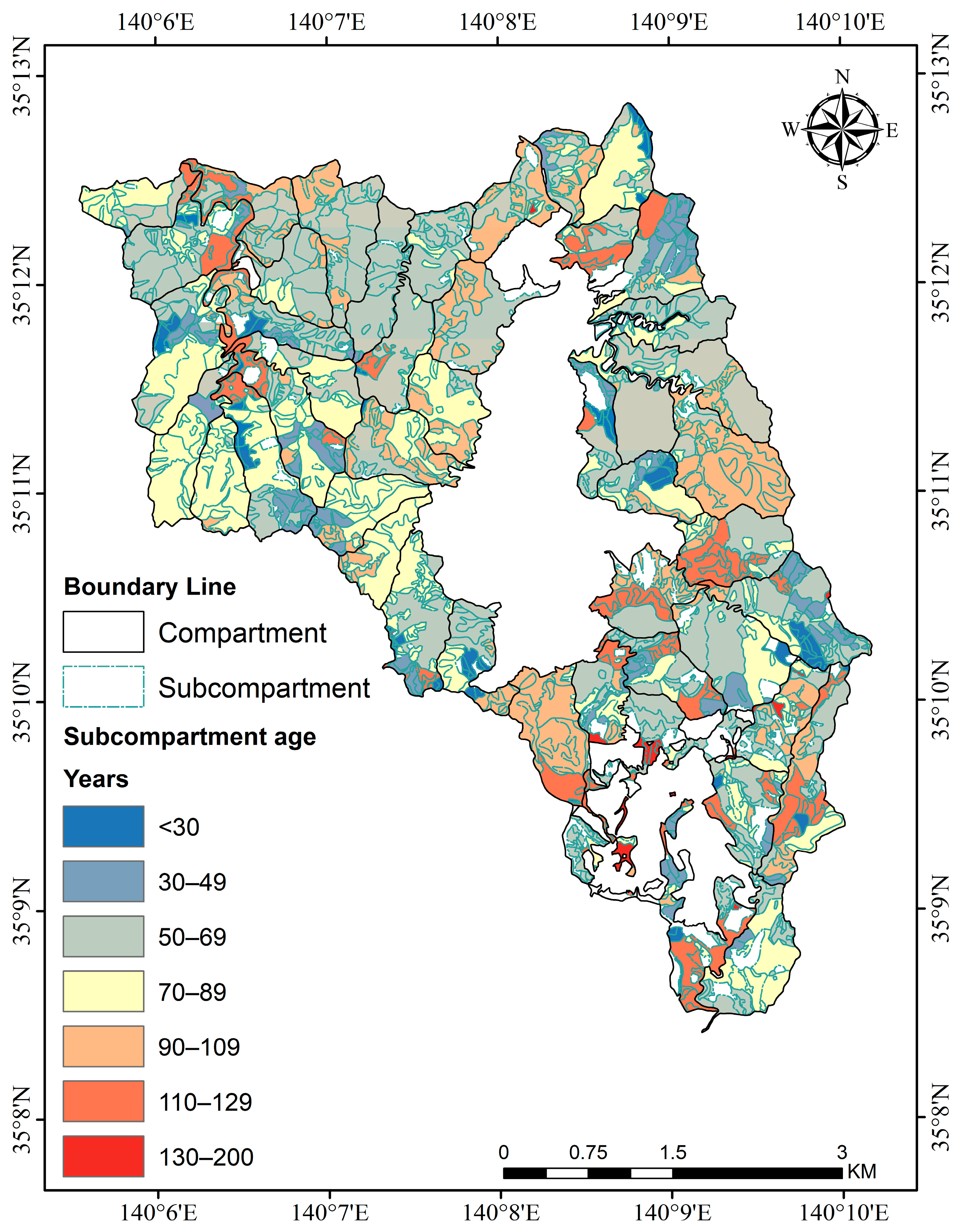
2.1. Study Area

The UTCBF (Figure 1) is located at the eastern end of the Boso Hills, in the southeastern Boso Peninsula (latitude 35°8′–12′N, longitude 140°5′–10′E, altitude 50–370 m). The mean annual temperature is 14.1 °C, and the mean annual precipitation is 2474 mm [52]. In order to clarify the position in the forest and provide management convenience, the forest management area is divided into forest compartments with 47 compartments in the UTCBF in total [53] (Figure 1). The subcompartment is a basic unit of management with similar structure trees and vegetation growing in similar site conditions [54,55], which is characterized with variables such as tree species, age, area, topography, and forest type for the UTCBF [53]; we uniformly named it as a forest stand in the following contents. The UTCBF has an area of 2160 ha and consists of warm temperate forest (a total number of 1602 forest stands), 267 ha of natural mixed forest with a total of 128 stands (ranging from 50 to 200 years old), 1117 ha of natural broad-leaved forest with a total of 545 stands (ranging from 50 to 200 years old), and 715 ha of plantation forest with a total of 929 stands (ranging from 13 to 200 years old) [43]. We omitted two other very small areas consisting of a stand type that was used for education and research, named the nursery and forest museum [52]. The natural mixed forest [56] is dominated by conifers and broad-leaved trees. The main tree species include Abies firma, Tsuga sieboldii, evergreen Quercus spp., and Castanopsis sieboldii [52]. The natural broad-leaved forest is dominated by C. sieboldii, evergreen Quercus spp., Zelkova serrata, and Acer spp. [52]. The conifer plantation is largely a monoculture of coniferous tree species (Cryptomeria japonica and Chamaecyparis obtusa) with a simple stand structure [52]. Since 1970, the coniferous and broad-leaved natural forests have been logged only to remove obstructive trees [57]. The natural broad-leaved forests were used as sources of fuelwood until the early 1960s but since 1980 have rarely been logged [57]. The UTCBF also includes well-protected compartments without human activity for the past 100 years, which are of high value, including for research [58]. The UTCBF has a complicated geology and steep mountains. The main soil type is brown forest soil, and the geological structure consists of marine deposits from the Neogene Period that are partly covered by non-marine deposits from the Quaternary Period [52]. In this study, carbon storage in the species-rich natural forest was estimated by combining natural broad-leaved forest with natural mixed forest, referred to below as natural forest.

2.2. Field Inventory Data

Field inventory data collected by UTCBF staff were used in this study. The plot distribution was as follows: 31 circular 0.1 ha plots established in old (≥100 years) C. japonica plantations were inventoried from September to December 2018 [59], 33 circular 0.03 to 0.1 ha plots containing young and middle-aged (10–119 years) conifer plantations were inventoried from September 2019 to September 2020, and 39 circular 0.03 to 0.1 ha plots were set up in natural forest and inventoried from January 2019 to October 2020 [43]. Within the plots, all trees with a diameter at breast height (DBH) of ≥5.0 cm (1.2 m above the ground) were measured using calipers or a measuring tape. For coniferous trees, the tree height (H) was measured using a Vertex IV (Haglöf, Sweden) or TruPulse 360 (Laser Technology, Inc., Centennial, CO, USA). The coordinates of the plot center were marked using a handheld GNSS receiver GPSMap 64 s (Garmin Ltd., Olathe, KS, USA). The tariff volumes of conifers (based on the DBH and H) and broad-leaved trees (based on the DBH) prepared for the UTCBF were used to calculate the merchantable tree volume. The CST was calculated using Equation (1) [60]:
CST = j { V j × D j × × B E F j × ( 1 + R j ) × C F }
where CST is the carbon stock in living biomass [Mg C ha−1], V is the merchantable volume [m3 ha−1], D is the wood density [Mg-d.m m–3], BEF (unitless) is the biomass expansion factor for the conversion of volume to total biomass, R (unitless) is the ratio of root biomass to aboveground biomass for a given tree species, CF is the carbon fraction of dry matter [Mg-C/t-d.m.], and j is the tree species. The values of CF were assumed to be 0.51 and 0.48 for conifers and broad-leaved trees, respectively. The CST equation and parameters of each variable were applied based on the National Greenhouse Gas Inventory Report of Japan [60]. For details about the biomass expansion factor, root-to-shoot ratio, wood density, and carbon fraction of tree species in Japan, see Appendix A Table A1.

2.3. RS Data

2.3.1. Data

Our RS dataset was obtained with a multi-spectral instrument (MSI) on board the Sentinel-2A. The images were orthorectified, georeferenced, and radiometrically calibrated into top-of-atmosphere (TOA) reflectance. It was acknowledged that Level 2A was the bottom-of-atmosphere corrected reflectance product; we could apply the atmosphere correction procedure to the L1A product with improved processing time and simpler implementation using the operational monitoring systems [61]. The simplified atmospheric correction procedure normalizes the top of the atmospheric corrections for aerosols considering the large uncertainties associated with complicated corrections, which are prone to errors in high biomass [62] and lead to information loss [61]. Level 1C had a varying spatial resolution over its spectral range, with four bands at 10 m (visible blue, green, red, and NIR bands), six bands at 20 m (four narrow bands in the VNIR vegetation red edge spectral domains B5, B6, B7, and B8a and two wider shortwave infrared bands SWIR-1 and SWIR-2), and three bands at 60 m (B1, B9, and B10) spatial resolution with a revisit frequency of 5 days (at the equator) and a 290 km swath width. The images used in this study were taken on 8 May 2017, when the cloud cover was <5%, and included all of the UTCBF area. The images were downloaded from the Copernicus Open Access Hub web platform (https://scihub.copernicus.eu/dhus/#/home, accessed on 19 February 2021) [63]. The DEM data, acquired on 10 December 2010, were generated using a GISMAP Terrain product (Hokkaido-Chizu Co. Ltd., Sapporo, Japan; https://www.hcc.co.jp/, accessed on 10 December 2010) and a JGD2000 datum geographical system with a 10 m grid resolution. The compatibility of the data with those from the JGD2011/Japan Plane Rectangular CS IX projection was achieved using the ArcGIS software version 10.8 (Esri Inc., Redlands, CA, USA) with defined projection commands. The main technical process used in this study is shown in Figure 2.

2.3.2. Data Pre-Processing

Atmospheric correction and the conversion of pixel values to surface reflectance was achieved by pre-processing the TOA image to level 2A at the bottom of atmosphere (BOA) reflectance image, using ESA’s processor Sen2Cor version 2.5.5 [64] algorithm in the Sentinel Application Platform (SNAP) (version 5.0). Of the 13 bands from Sentinel-2A [63], 10 (three visible, a near-infra-red band, four narrow bands in the VNIR vegetation red edge spectral domain, and two wider SWIR bands (SWIR-1, and SWIR-2)) were extracted for pre-processing and resampled to 10 m spatial resolution using the nearest-neighbor method in the SNAP geometric operation tool.

2.3.3. Ancillary Variables
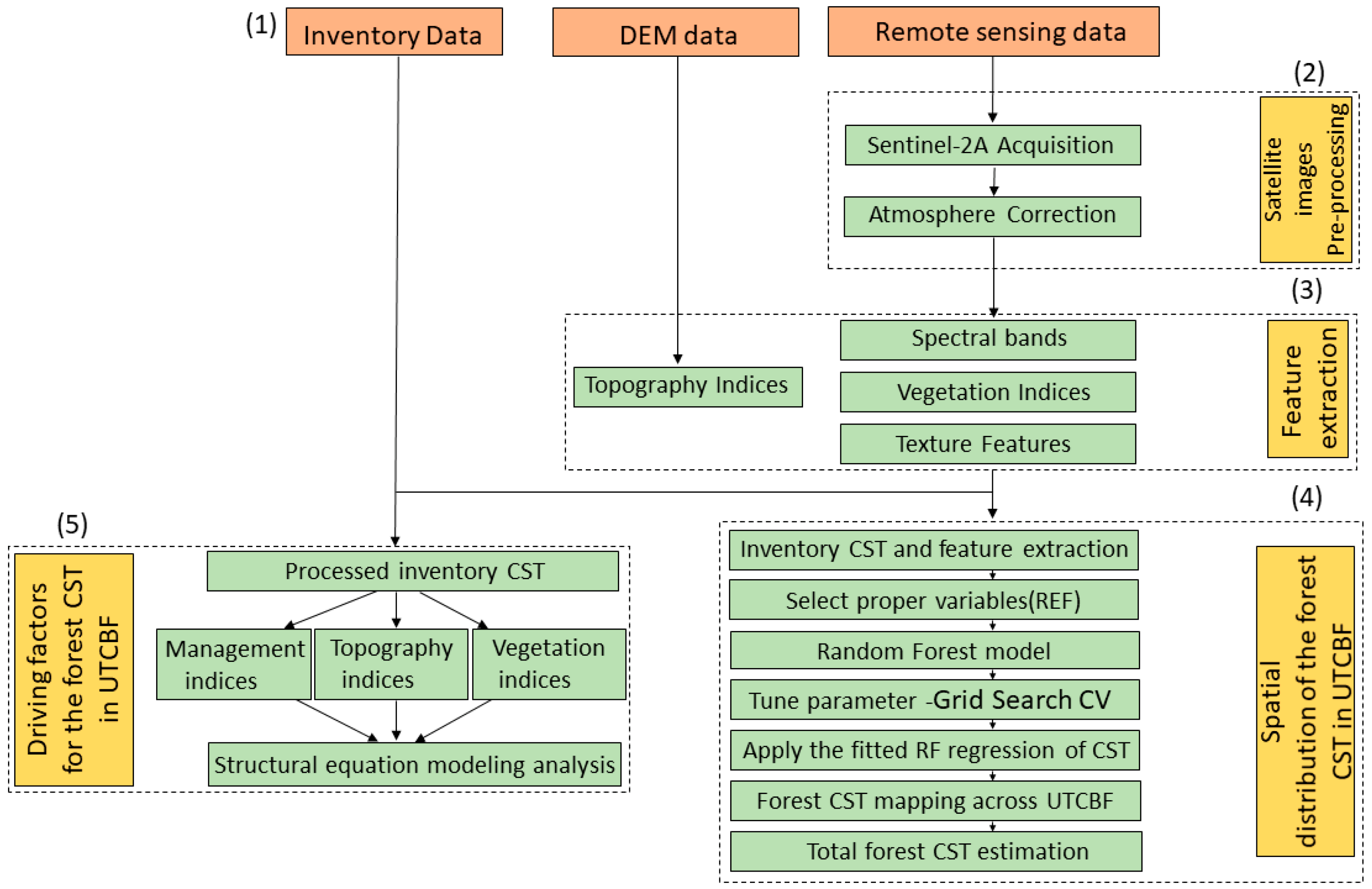
The Sentinel-2A bands were used to create the vegetation indices (NDVI, EVI, and RVI) [24,29] datasets (Table 1). Topographic conditions and environmental factors play important roles in the generation and location of forest species and types [21,29,40,41,51] (Table 1). All RS data were set up according to the JGD2011/Japan Plane Rectangular CS IX projection coordinate system. The texture features [65] (Table 1) were extracted from the Sentinel-2A-based bands using the gray-level co-occurrence matrix (GLCM), calculated with Envi version 5.5 (L3Harris Geospatial Solutions, Broomfield, CO, USA) and including the variance and contrast. The GLCM variance measures the heterogeneity variance when the gray value of the image differs from its mean. The GLCM correlation measures the linear dependencies of the images; there is a linear relation of the adjacent pixels when higher linear correlation values are represented [66].
The topographic indices, including solar radiance, elevation, slope angle, aspect, curvature, and topographic wetness index [51], were calculated using Envi software (L3Harris Geospatial Solutions, Broomfield, CO, USA) and a 10 m grid DEM from the GISMAP Terrain product.

2.4. Data Analysis

2.4.1. Feature Selection

The importance of various features in the outcome of the prediction model was determined by automatically ranking the relative importance of all predictor variables. The Gini importance [37] of each variable was determined by calculating decreases in the impurity of all nodes in which the variable was split. The impurity of the decreases was weighted by the fractions in the nodes and then averaged over all trees [37] using a reduction in the mean squared error (MSE) as the criterion.

2.4.2. Carbon Stock Prediction by Machine Leaning

RF is an ensemble-based machine learning model in which a multitude of decision trees are selected based on a majority vote. RF uses the bootstrapping technique to reduce model variance without increasing bias while increasing the accuracy and reducing overfitting during classification and regression. RF tests a random subset of the explanatory variables for each node to select the optimal split from a set of predictors [74]. It increases the diversity of individual decision trees, reduces overfitting, and improves the ensemble model.
Python 3.6.7 libraries scikit-learn 0.24.2 [75] and the GridSearchCV function in the sklearn.model_selection package were applied to train the model pipelines. A dictionary was established to store the parameters that needed to be searched, after which the necessary model fitting and selection of the output best parameters were performed using GridSearchCV for grid search and cross-validation. The training dataset was split into equal numbers of subset N-folds. The model was then iteratively fitted N times, with the data trained each time on (N–1) folds, after which the remaining one-fold (hereafter referred to as the validation data) were evaluated. A different fold was evaluated each time, and the cross-validation root mean square error (RMSE) performance was averaged on each one to finally derive the lowest cross-validation RMSE as the best trained model pipeline and thus the final validation metrics for the model. Hyperparameter tuning automatically performed iterations of this entire N-fold cross-validation process, using different model settings each time. The final hyperparameters were (1) n_estimators, defined as the number of decision trees, set at 500; (2) max_features, defined as the largest number of features for each decision tree and set at auto; and (3) maximum depth, defined as the maximum depth of the decision tree, set at 9. The field inventory plots were randomly split into 80% and 20% for the training and testing samples, respectively, using the train_test_split function in the sklearn.model_selection package for Python 3.6.7 libraries.
The model used the RS data to predict the CST of each testing pixel located within the inventory plots, with each pixel representing an area of 0.01 ha. The resulting CST values were summed to obtain the total CST density, which when divided by the plot area allowed their expression as Mg C ha−1. This study was based on a Sentinel-2A 10 m spatial resolution DEM dataset, DEM-based topography indices, Sentinel-2A spectral-based vegetation indices, textures, and field inventory data to model the CST across the UTCBF. Four models differing in their RS data composition were compared: (1) Sentinel-2A spectral bands only; (2) Sentinel-2A spectral bands with topographic indices; (3) Sentinel-2A spectral bands, topographic indices, and vegetation indices; and (4) Sentinel-2A spectral bands, topographic indices, vegetation indices, and Sentinel-2A-based textures. Calibration and validation errors were used to evaluate the performances of the different CST models, including the RMSE, coefficient of determination (R2), relative RMSE (rRMSE), bias, and %bias (bias/mean value of observations) [23,74]. Higher R2 and lower RMSE, rRMSE, bias, and %bias values indicated greater accuracy of the prediction model.

2.4.3. Carbon Stock Mapping by Forest Type and Stand Age

The UTCBF has well-protected natural forests and well-managed conifer plantation forests containing trees of different age classes [41]. Identifying forest CST by forest type and stand age can provide knowledge on the magnitude and spatial distribution of this resource in a similar forest management policy. The CST prediction model was applied to show the spatial distribution of the CST at a spatial resolution of 10 m using RS datasets of different compositions for places outside the field survey area. Data preparation, analyses, and geo-visualization were carried out using the ArcGIS software version 10.8 (Esri Inc., Redlands, CA, USA) and Python with the GDAL 2.4.1 package. RS data-based wall-to-wall prediction maps were used to summarize the total estimated CST by forest type and stand age using the ArcGIS software version 10.8 and a zonal statistics geo-processing tool. The CST per pixel was calculated, and the values were then averaged to obtain the CST and carbon density by forest type and stand age [4], as described in forest management stand information for the UTCBF. The conventional estimation of the CST as a function of forest type and stand age (Figure A1) was calculated as follows (2):
T stand = A stand × A v stand
where T s t a n d ,   A s t a n d , and A v s t a n d are the total forest type CST for each stand, the stand area, and the average CST for each forest type and stand age according to the inventory plot, respectively.

2.4.4. Factors Driving the Spatial Distribution of Carbon Stock

As a piecewise structural equation model (pSEM) is built using a series of structured equations and implemented with linear modeling functions, it is independent of the data distribution and thus allows for non-normal distributions, hierarchical structures, and different estimation procedures. The path diagram is translated to a set of linear structural equations that are evaluated separately [76,77]. The piecewiseSEM package in R version 4.2.0 [77,78,79] was used to evaluate the association between topographic factors (aspect, curvature, and DEM), vegetation index factors (EVI and NDVI), forest management factors (forest type, stand age, and stand density), and CST, resulting in information that could support forest management. The model was separated into composite variables to test the collinearity of all influential factors and then included in the SEM. The robustness of the relationship between CST and its driving factors was confirmed using marginal and conditional contributions to account for the random effects of the inventory plots. Finally, Fisher’s C-test (0.05 < p < 1.00) was used to obtain the Akaike information criterion (AIC), which together with the Bayesian information criterion (BIC) was used to confirm the goodness of modeling. The significance (p < 0.05) was used to identify the optimal model among those developed in this study [78].

3. Results

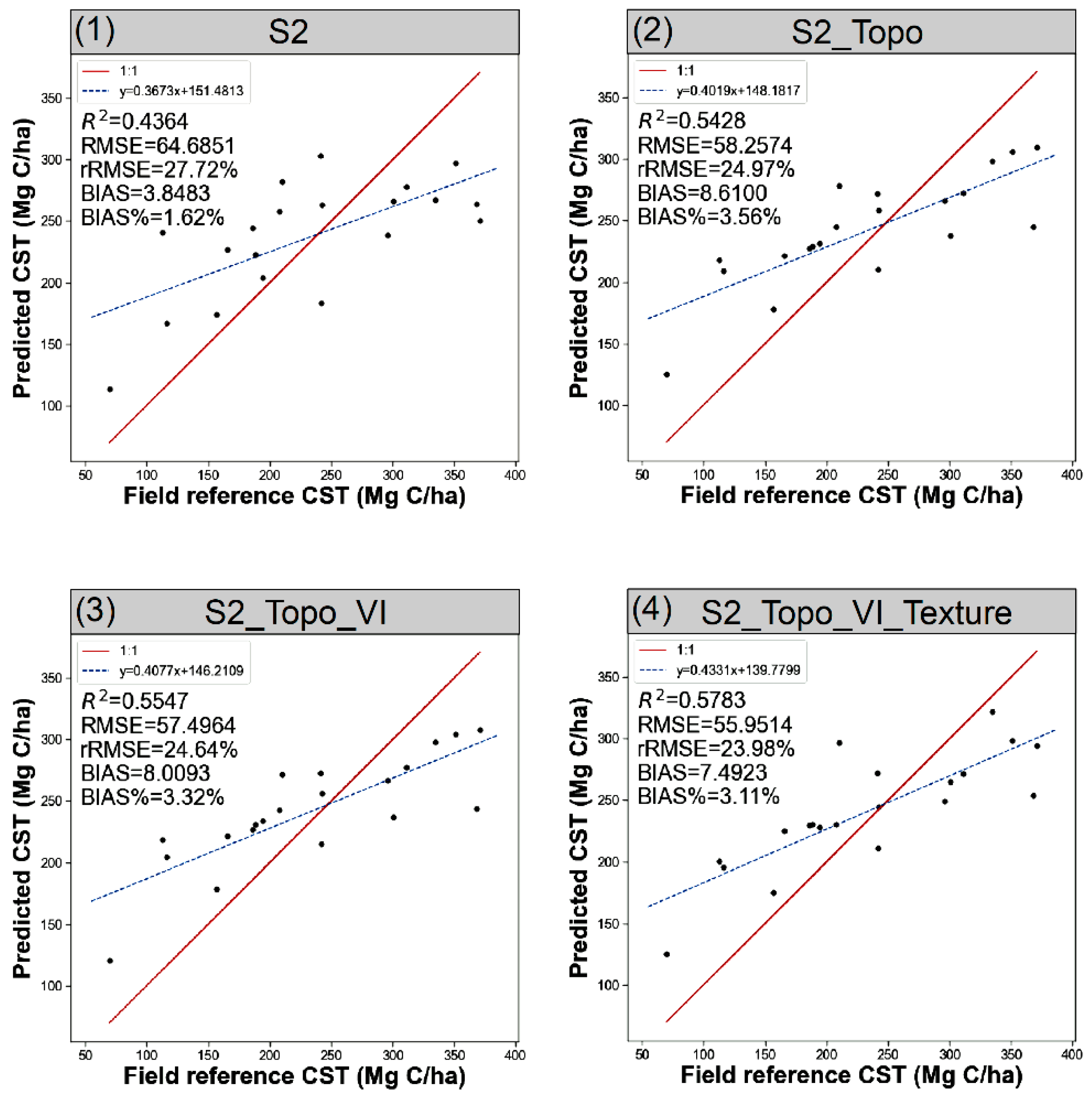
3.1. RS Dataset and Regression Modeling for Carbon Stock

Figure 3 presents the CST predicted by the four models. Among the models, the best-performing model was that based on the Sentinel-2A spectral bands in combination with the topography indices, vegetation indices, and B12-derived textures (S2_Topo_VI_Texture), as indicated by an R2 of 0.5783, an RMSE of 55.9514 Mg C ha−1, an rRMSE of 23.98%, a bias of 7.4923, and a %bias of 3.11% [Figure 3(4)]. The model with the poorest performance was that consisting only of the Sentinel-2A RS dataset [R2 = 0.4364, rRMSE = 27.72%; Figure 3(1)]. The inclusion of topographic indices (S2_Topo) improved the R2 of the latter model by 24.38% (R2 = 0.5428, rRMSE = 24.97%). The addition of vegetation indices to the topographic and spectral information (S2_Topo_VI) improved the model prediction accuracy only slightly (R2 = 0.5547, rRMSE = 24.64%).

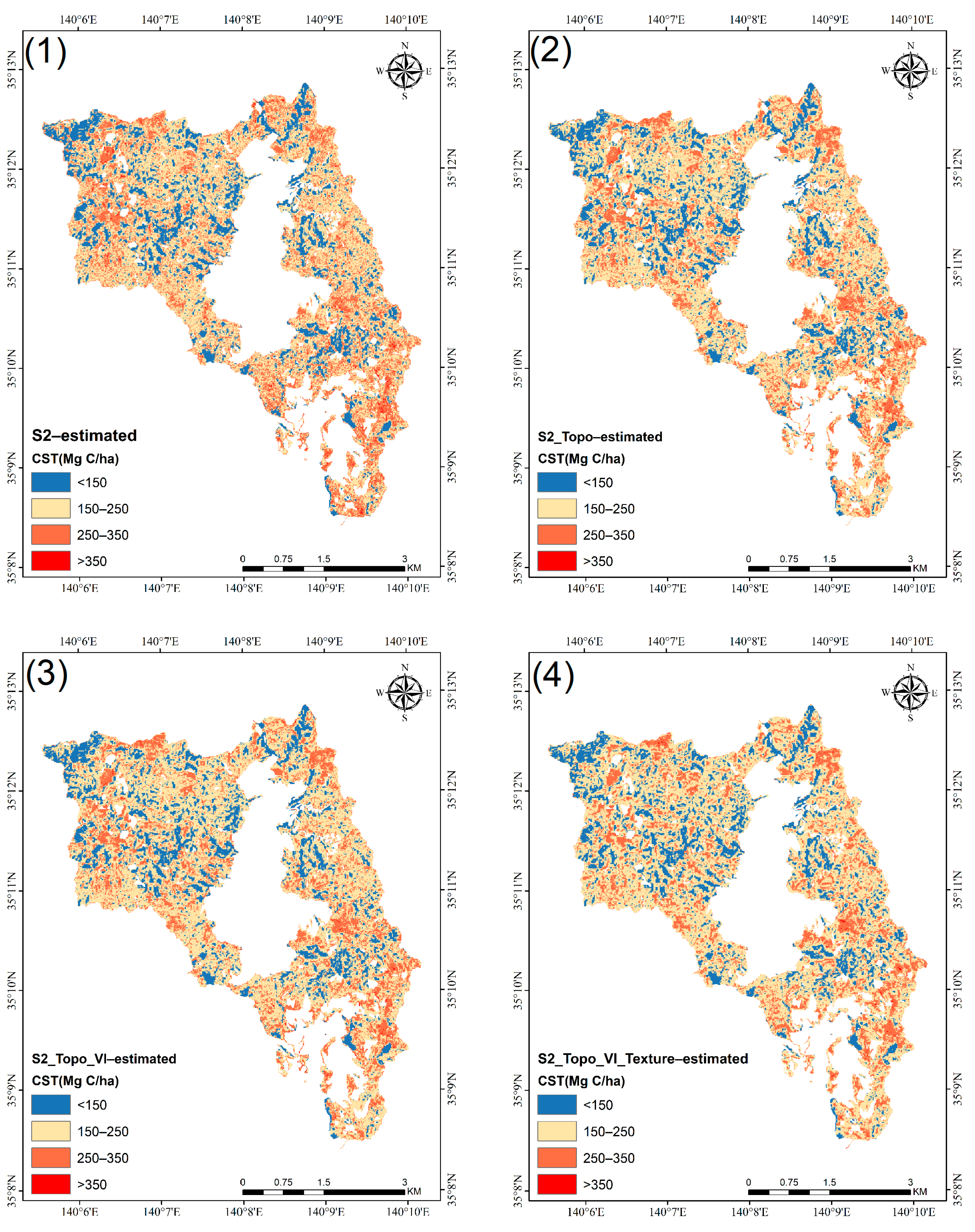
3.2. Mapping of Forest Carbon Stock over the Study Area

Figure 4 shows the wall-to-wall map of the spatial CST distribution within the study area as predicted by the four RS datasets and by the conventional estimation method (Figure A2). The RS-estimated CST values were heterogeneous across the different forest stands, whereas the conventionally estimated CST, which is based on the average value of the inventory plot, failed to capture fine-scale spatial variations. The CST values ranged from 48.02 Mg C ha−1 to 432.49 Mg C ha−1 for S2 [Figure 4(1)], from 64.54 Mg C ha−1 to 403.38 Mg C ha−1 for S2_Topo [Figure 4(2)], from 62.92 Mg C ha−1 to 405.40 Mg C ha−1 for S2_Topo_VI [Figure 4(3)], and from 73.66 Mg C ha−1 to 418.04 Mg C ha−1 for S2_Topo_VI_Texture [Figure 4(4)]. Figure 5 shows the pixel percentages of the different CST value ranges, and Table A2 shows the total amount of CST of different categories. In the CST spatial distribution maps [Figure 4(2)–(4)], the percentage of pixels predicting a CST more than 350 Mg C ha−1 was largest in the southeast plantation forest. The largest percentages of RS prediction pixels were in areas with CST values of 150–250 Mg C ha−1, which included both natural and plantation forests, followed by areas with CST values of 250–350 Mg C ha−1. In the S2_Topo_VI_Texture prediction map, 43.60% (19,552,259 Mg C ha−1) and 19.76% (8,860,915 Mg C ha−1) of the study area had CST values of 150–250 Mg C ha−1 for natural forest and plantation forest, respectively. CST values above than 350 Mg C ha−1 were predicted for 0.02% (8809 Mg C ha−1) and 0.21% (91,733 Mg C ha−1) of the natural forests and plantation forests, respectively. CST values of less than 150 Mg C ha−1 occurred in 8.89% (19,552,259 Mg C ha−1) of natural forests but only 1.15% (513,535 Mg C ha−1) of plantation forests. In addition, from the Appendix A Table A2, we can find that the total carbon stock of the natural forest is higher than that of the plantation forest for all the experiments.

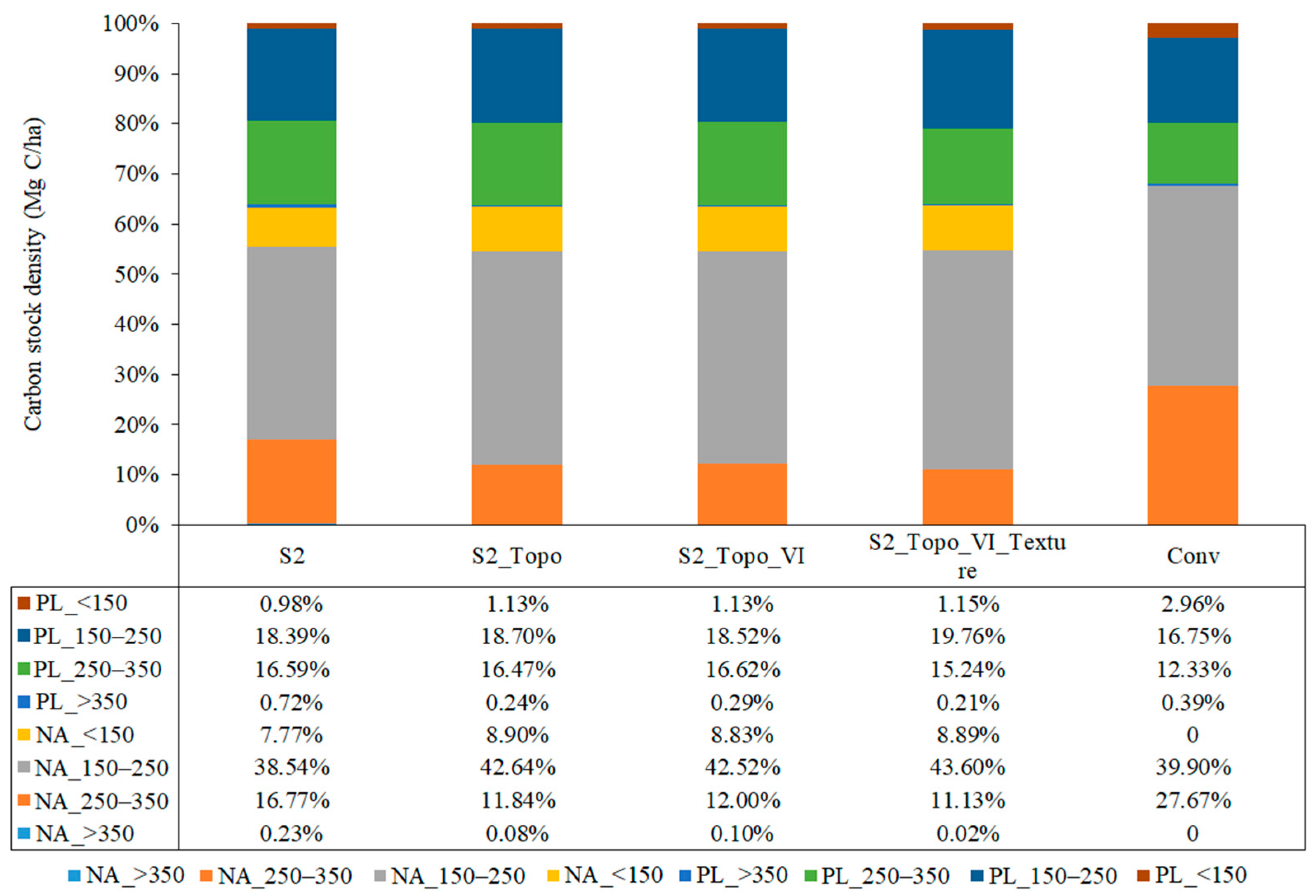
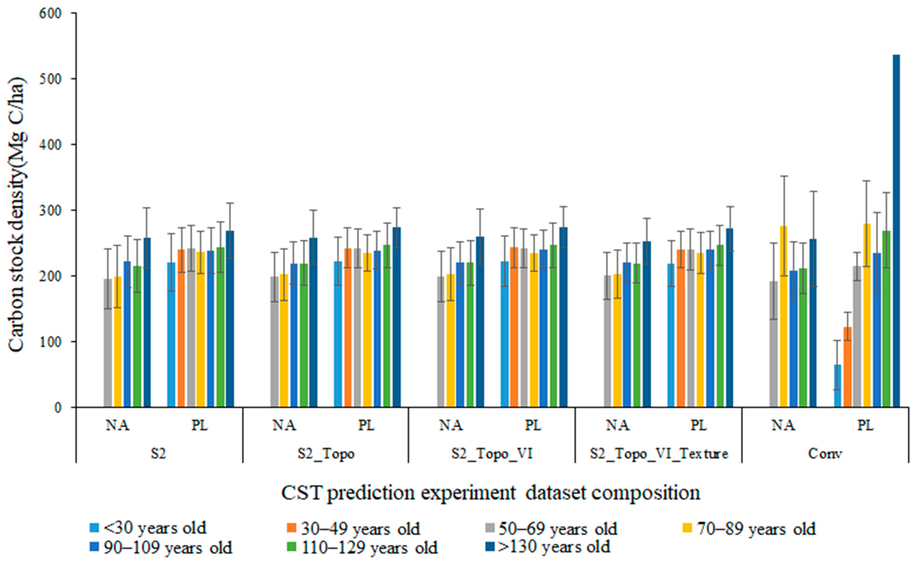
3.3. Calculation of Mapped CST by Forest Type and Stand Age

Figure 6 and Table A3 show the predicted CST density by forest type and stand age class as extracted from the four RS models and the CST determined according to the conventional method. For the conifer plantation, the CST predicted by the conventional method increased with stand age, except for stands 70–89 years of age, for which the value was extremely high (284 Mg C ha−1). The RS-predicted CST also increased with stand age, except for plantation forests 30–69 years of age and natural forests 110–129 years of age. For conifer plantation forests, the Sentinel-2A-based RS datasets overestimated the CST for stand ages <70 years and underestimated the CST for stand ages >70 years old compared with the conventional method. For natural forests, Sentinel-2A-based RS underestimated the CST for stand ages >70 years and overestimated the CST for stand ages <70 years and >130 years. The RS model underestimated the CST for very old plantation forests and was limited in its prediction of CST when the forest density was high or the vertical structure of the natural forest was dense.

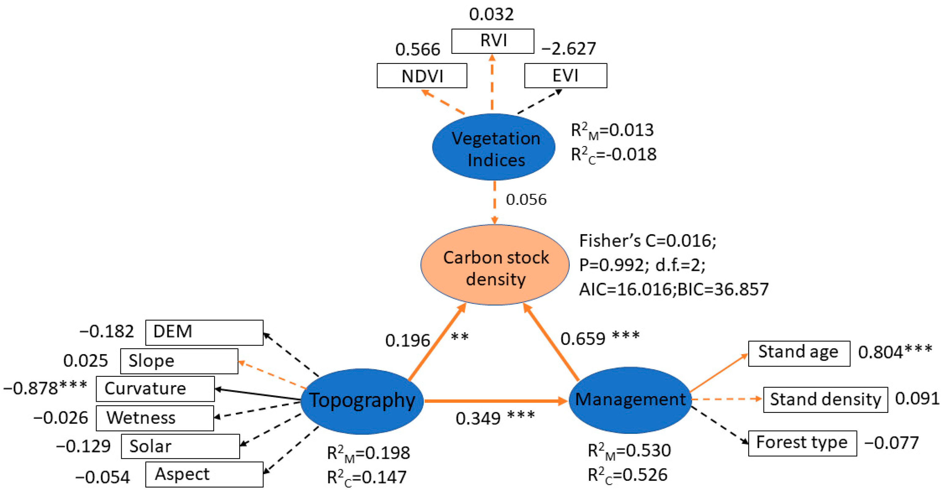
3.4. Relative Importance of Factors Driving the Spatial Distribution of Carbon Stock

The optimal predictors for modeling CST in the UTCBF were derived from a determination of the Gini important variables. Figure 7 shows the importance ranking of the four RS experiments. Compared with spectral bands and DEM information, SWIR-2, solar, and SWIR-2-based textures (variance and correlation) were better predictors in CST modeling, followed by topography indices, such as aspect, slope, and wetness. The importance of other spectral bands, such as VNIR (B5 and B7), NIR (B8 and B8a), and the green band (B3), did not differ greatly. EVI and NDVI were the least important variables in the CST prediction model.
Figure 8 shows the direct and indirect effects of the factors on CST density spatial variation according to the pSEM. The model explained 57% of the direct and 12% of the indirect variations in CST density. Management factors had a direct and significantly positive effect on CST density (0.659, p < 0.001) as did topographic factors (0.196, p < 0.01). The latter also had an indirectly positive effect on CST density, through forest management factors (0.349, p < 0.001). Stand age acting through management factors had a strong, positive (0.827) effect on CST density for stand ages 50–200 years for natural forests and 13–200 years for plantation forests. Curvature, as a topographic factor, had a significantly strong negative effect (−0.878, p < 0.001) on CST density. DEM, wetness, solar, and aspect had a negative but not significant influence on CST density. The vegetation indices NDVI and RVI had a positive effect on CST density, whereas the EVI had a negative effect.

4. Discussion

4.1. Model Performance for Forest Carbon Stock

This study shows that the accuracy of CST prediction for natural forests and plantations using Sentinel-2A data (R2 = 0.4364, RMSE = 64.6851 Mg C ha−1) was similar to that of previous studies (R2 = 0.4197, RMSE = 31.016 Mg C ha−1) [80], with the prediction accuracy increased by combining Sentinel-2A spectral bands with SWIR-2-based textures, vegetation indices, and topographic indices (R2 = 0.5783, RMSE = 55.95 Mg C ha−1). Previous research [34,81,82,83] showed that topography indices, vegetation indices, and textures could effectively improve the accuracy of biomass estimations based on Sentinel-2A datasets. In a study in Myanmar [21], this approach resulted in an R2 of 0.52 and 34.72 t of aboveground biomass/ha. Topographic features are closely related to forest type distribution [29,80]. Mountainous topography accounts for the micro environmental heterogeneity of habitat and resource (light, water, and soil nutrients) availability for the different forest types [84]. Spectral bands in the red edge and shortwave infrared ranges are highly sensitive to vegetation [85]. Spectral bands (B2 and B3) have a reflectance peak at wavelengths between 440 nm and 570 nm [86], B3 and B4 are sensitive to chlorophyll, and SWIR-1 and SWIR-2 indicate the moisture content of vegetation [34,81]. Accordingly, the combination of spectral and terrain information with vegetation indices improved CST model accuracy and eliminated the saturation problem [22,87,88,89]. In previous studies, optimal RS data were combined with synthetic aperture radar (SAR) or LiDAR data to improve prediction accuracy [29,31,80,90,91]. Li et al. [92] showed that the combination of Sentinel-2 and PALSAR2 datasets performed better (R2 = 0.37, RMSE = 98.63 Mg C ha−1) than either dataset alone in a C. japonica forest, by eliminating the sensitive saturation of microwave RS imagery. Zhang et al. [91] combined optical image Landsat 8 data with LiDAR, which resulted in an R2 of 0.935 and an RMSE of 15.67 Mg C ha−1. Although we lack tree height data, the compensation of DEM data can improve the CST prediction accuracy to some extent and alleviate the influence of mountain topography.
The CST values predicted by all RS-based models (Figure 3) were overestimated for relatively low values and underestimated for relatively high values, as is often the case in RS-based CST estimation [24,93,94]. This can be explained as follows. First, the selection of a sufficient number and appropriate inventory plots in this study was limited by the mountainous terrain, which also hampered extensive field measurements; consequently, the inventoried plots were not always representative of the CST density value range of the trees in the research site [95,96], as there were fewer low- and high-CST-density plots than medium-CST-density plots, resulting in overestimation and underestimation. Second, the satellite image pixel size may not have been optimal for the dimensions of the sampled plots [97]. Third, optical RS data are not sensitive to very-high-density-CST forests, and the lack of canopy penetration prevents the extraction of information on the vertical structure of the forest or on tree height, which is important for the calculation of CST density, resulting in saturation problems [94,98,99]. Fourth, variations across the plots with respect to tree species composition [94] and forest canopy structure [100,101] may have reduced the estimation accuracy; in the study area, the upper-story conifer trees A. firma accounted for more than half of the conifer mixed forest with high CST densities. This was also the case for the composition of tree species with respect to the natural mixed forest, and natural broadleaved forests are similar, whereas the heterogeneity of the natural forest increased with age, as C. sieboldii and evergreen Quercus spp. became increasingly large and dominant and intermixed with small Eurya japonica var. japonica and Cleyera japonica Thunb [43].

4.2. Mapping of CST

The conventional method (Figure A2) averaged the CST density at the stand level as it could not account for the variance in the canopy gap and in tree species, whereas the RS-based wall-to-wall prediction map detected all the pixels within each stand and was thus able to capture the spatial heterogeneity of the forests. Forests with a high CST density (>250 Mg C ha−1) were concentrated in the northwest part of the study area, and those with a medium CST density (150–250 Mg C ha−1) were concentrated in the northern part, as determined from the conventional method. The conventional and RS-based maps similarly identified the position of low-CST-density (<150 Mg C ha−1) forests, whereas the RS-based CST prediction map (Figure 4) allowed the discrimination of changes in CST in terms of terrain and forest type. Forests with a high CST density (>250 Mg C ha−1) were mainly located in low elevation and flat areas and mainly consisted of plantation forests in the southeast and northwest. Forests with a low CST density (<150 Mg C ha−1) were typically young natural forests located in the northwest and northeast and at a relatively high altitude. In these areas the soil is drier, shallower, and less fertile due to the lower pH and lower concentration of nutrients such as phosphorous and potassium, such that the growth of evergreen broad-leaved trees is limited [41,58]. However, despite the disparities between the different models, the value ranges indicate that the UTCBF is mostly (80%) characterized by medium CST values (150–350 Mg C ha−1). However, CST densities may be >350 Mg C ha−1 and as high as 432.49 Mg C ha−1 [44], as described in a previous study [93]. Plantation forests have larger areas of CST densities between 350 and 500 Mg C ha−1 than found in natural forests. High-CST-density C. japonica and C. obtusa plantations are widely distributed in Japan [102], and both species dominate in their well-managed, old (≥100 years) plantations in the UTCBF. The high carbon biomass production of these trees results in high CST densities [43].

4.3. Calculation of CST Maps by Forest Type and Stand Age

In the study area, plantation forests had a higher CST density than natural forests for all stand ages (Table A3). Zhao [13] similarly found that the CST density of plantation forests increases with stand age. By contrast, in tropical areas, natural forests acquire a higher CST density than plantation forests [4] due to the abundant rainfall and temperature suitable for their growth. In areas of Japan such as Kanto, Kinki, Shikoku, and Kyushu [5,15], the CST density is higher in boreal or subalpine coniferous forests than in natural forests as the typical oceanic climate of Japan, with abundant precipitation and warm temperatures, favors the fast growth of conifers. For the four RS prediction models, plantation forests became saturated at a CST density >230 Mg C ha−1, perhaps due to the canopy vacancy gap between the rows and columns of the plantations [32] as well as the influences of shadow and terrain [103]. Our study also shows that the combination of RS data with DEM and texture indices can mitigate underestimations in high-CST-density forests (and overestimation in young forests) and thus improve the accuracy of CST mapping, despite the documented deficiencies of LiDAR data with respect to forest structure and tree height [32,104]. Moreover, our method can be applied universally, especially in mountainous terrain, owing to its use of open source RS datasets. In the vegetation indices, the use of Sentinel-2A red edge bands mitigated the vegetation biomass saturation problem. Because the UTCBF has a typical oceanic climate with abundant rainfall and adequate vegetation moisture, SWIR bands can be used to assess the moisture content and biomass of its vegetation features [21,81]. Although forest inventory data [100] are considered reliable and are a fundamental source of CST density data for RS-based model training, plot survey data may be biased, resulting in uncertainty. Our inventory CST was much higher than that of the national inventory [5] made up of stands of the same age, as was also the case in other studies [3,105].

4.4. Relative Importance of Factors Driving the Spatial Distribution of Carbon Stock

Our study also demonstrates the critical role of the B12 (SWIR band) and terrain data in shaping CST predictions. For the S2_Topo_VI_Texture dataset, 75% of the respective model was explained by B12, B12-based textures, solar, red band, aspect, slope, and wetness. The high explanatory power of B12 is due to its ability to reflect vegetation water content and stand structure complexity [83,93], such that it is well suited to CST prediction in a climate such as that of the UTCBF. Dang et al. [22] also showed a strong relation between B12 and field-measured CST [23]. The second most critical variable in CST modeling was solar, most likely due to its direct influence on photosynthesis. The pSEM further revealed how the three groups of factors (topography indices, forest management, and vegetation indices), and especially curvature and stand age, drive the spatial distribution of CST density in the UTCBF. The topography indices directly affected the forest CST and indirectly affected the forest CST adjusted for forest management. Curvature [106], which influences water migration and accumulation by gravity [107,108] and thus nutrient levels, had a significantly negative effect on CST, whereas slope had a positive impact on forest CST, in agreement with a previous report [109]. Forest species composition and distribution are affected by topographic factors through runoff, erosion [110], light condition [111], slope [108], and the features of the regional environment. The strong positive relationship between stand age and CST indicates that CST continues to accumulate in live biomass as the forest ages [45,112] and that old, well-protected natural and plantation trees in the UTCBF continue to play an important role in carbon storage. The strong positive relationship between stand age and CST is supported by our RS-based predictions, according to which CST increased with forest stand age for both forest types (Figure 6 and Table A3). The slightly positive effect of stand tree density on CST reflects the fact that a high stand density can optimize resource utilization through canopy packing [84]. A high tree density also supports an optimal forest microenvironment and nutrient supply, but if it is too high, it may have a negative effect on CST due to competition for light and nutrients.

5. Conclusions

The use of RS dataset and DEM data to assess forest CST spatial variation can provide technical support to maintaining the carbon budget and to sustainable forest management. To our knowledge, this is the first study to estimate the impact of three categories of factors (topography indices, forest management, and vegetation indices) in driving the spatial distribution of CST at a landscape scale.
The integration of Sentinel-2A datasets with DEM-based topographic indices, vegetation indices, and spectral band-based textures to estimate the forest CST in the UTCBF using the RF method resulted in a CST prediction with relatively high accuracy (R2 = 0.5428, rRMSE = 24.97%). According to this mapping approach, the CST was larger in plantation forests than in natural forests and increased with stand age. The majority of the predicted CST values were in the range of 150–350 Mg C ha−1. Stand age, as a management factor, had a significant and strongly positive effect (0.827) on CST density, while curvature, as a topography factor, had a significant and strongly negative (−0.878) effect on CST density. Our RS-based approach can improve estimation and quantification of CST for different forest types and stand ages and thereby contribute to achieving sustainable forest management. Saturation and uncertainty in CST modeling due to the inherent limitations of the inventory plots and the lack of forest height information are problems that remain to be resolved.
Due to the limitation of only using a single-date remote sensing product for CST prediction, in the future, the state of art multi-modal fusion deep learning methods [113] and the generation of multi-modal and multi-temporal RS datasets [32,114] should be considered to be used to build a robust CST estimation model in the circumstance of lacking enough inventory plot data and canopy height data. Meanwhile, it is also an interesting topic to examine the changes in CST by analyzing the Sentinel-2A images taken before and after some disturbances such as the typhoon event to check the influence of the natural disturbance to the forest [115].

Author Contributions

Conceptualization, methodology, formal analysis, and writing (original draft preparation), H.P.; resources, supervision, and writing (review and editing), T.O.; writing and major review and editing, S.T.; review and editing, T.H. All authors have read and agreed to the published version of the manuscript.

Funding

This study was partially supported by the Japan Society for the Promotion of Science (JSPS) KAKENHI Grant Number [JP18K05742].

Data Availability Statement

Not applicable.

Acknowledgments

The authors would like to thank the technical staff from the UTCBF for their contribution to the forest type interpretation and inventory data collection, and the authors would like to thank Keisuke Toyama of the University of Tokyo for their kind help through the provision of professional information and comments about this paper. This research is partially supported by the Initiative on Recommendation Program for Young Researchers and Woman Researchers [2023-A-027], Information Technology Center, The University of Tokyo.

Conflicts of Interest

The authors declare no conflict of interest.

Appendix A

Figure A1. Forest subcompartment age map.
Remotesensing 15 01997 g0a1
Figure A2. Spatial distribution of the CST predicted using the conventional method.
Remotesensing 15 01997 g0a2
Table A1. Biomass expansion factor, root-to-shoot ratio, wood density for tree species, and carbon fraction [60].
BEF>20 [-]R [-]D [t-d.m./m3]CF [t-C./t-d.m]Note
Conifer treesJapanese cedar1.230.250.3140.51
Hinoki cypress1.240.260.407
Sawara cypress1.240.260.287
Japanese red pine1.230.260.451
Japanese black pine1.360.340.464
Hiba arborvitae1.410.200.412
Japanese larch1.150.290.404
Momi fir1.400.400.423
Sakahaline fir1.380.210.318
Japanese hemlock1.400.400.464
Yezo spruce1.480.230.357
Sakhaline spruce1.670.210.362
Japanese umbrella pine1.230.200.455
Japanese yew1.230.200.454
Ginkgo1.150.200.450
Exotic conifer trees1.410.170.320
Other conifer trees1.320.340.352Applied to Hokkaido, Aomori, Iwate, Miyagi, Akita, Yamagata, Fukushima, Tochigi, Gunma, Saitama, Niigata, Toyama, Yamanashi, Nagano, Gifu and Shizuoka prefectures
1.360.340.464Applied to Okinawa prefecture
1.401.400.423Applied to prefectures other than above
Broad leaf treeJapanese beech1.320.260.5730.48
Oak (evergreen tree)1.330.260.646
Japanese chestnut1.180.260.419
Japanese chestnut oak1.320.260.668
Oak (deciduous tree)1.260.260.624
Japanese popular1.180.260.291
Alder1.250.260.454
Japanese elm1.180.260.494
Japanese zelkova1.280.260.611
Cercidiphyllum1.180.260.454
Japanese big-leaf1.180.260.386
Maple tree1.180.260.519
Amur cork1.180.260.344
Linden1.180.260.369
Kalopanax1.180.260.398
Paulownia1.180.260.234
Exotic broad leaf trees1.410.160.660
Japanese birch1.200.260.468
Other broad leaf trees1.370.260.469Applied to Chiba, Tokyo, Kochi, Fukuoka, Nagasaki, Kagoshima, and Okinawa prefectures
1.330.260.646Applied to Mie, Wakayama, Oita, Kumamoto, Miyazaki, and Saga prefectures
1.260.260.624Applied to prefectures other than above
BEF: biomass expansion factor (20 = age class); R: root-to-shoot ratio; D: wood density; CF: carbon fraction.
Table A2. Summary of the CST for each value category using different methods.
CST (Mg C ha−1)S2 (Mg C)S2_Topo (Mg C)S2_Topo_VI (Mg C)S2_Topo_VI_Texture (Mg C)Conv (Mg C)
PL <150432,676504,370504,886513,5351,374,287
PL 150–2508,164,0408,373,4858,301,6718,860,9157,789,185
PL 250–3507,363,4677,376,4107,446,2326,831,9545,734,396
PL >350320,299108,915128,20691,733179,358
NA <1503,446,3373,985,7763,958,5323,990,232-
NA 150–25017,104,83019,090,12619,056,02319,552,25918,551,958
NA 250–3507,441,8475,300,9745,378,7464,991,93812,865,968
NA >350103,64735,92043,1158809-
Total_PL16,280,48216,363,18016,380,99516,298,13715,077,226
Total_NA28,096,66128,412,79628,436,41628,543,23831,417,926
Total44,377,14344,775,97644,817,41144,841,37546,495,152
Conv: conventional estimation method; S2: Sentinel-2A series dataset (S2); S2_Topo: Sentinel-2A bands fused with topography indices; S2_Topo_VI: Sentinel-2A bands fused with topography indices and vegetation indices; and S2_Topo_VI_Texture: Sentinel-2A bands fused with topography indices, vegetation indices, and textures. PL: plantation forest; NA: natural forest.
Table A3. Map of CST density by stand age class for natural forests and conifer plantations. NO: not observed in the inventory data.
Stand Age (Years Old)S2 (Mg C ha−1)S2_Topo (Mg C ha−1)S2_Topo_VI (Mg C ha−1)S2_Topo_VI_Texture (Mg C ha−1) Conv (Mg C ha−1)
NAPLNAPLNAPLNAPLNAPL
<30NO220.53
(44.33)
NO221.84
(37.20)
NO221.75
(37.78)
NO218.43
(34.15)
NO63.89
(38.11)
30–49NO239.48
(34.34)
NO242.38
(30.81)
NO242.74
(31.03)
NO239.41
(28.05)
NO122.61
(21.61)
50–69195.07
(45.77)
241.96
(34.92)
198.21
(37.78)
241.73
(29.74)
198.45
(38.13)
242.13
(29.90)
199.83
(35.37)
239.49
(31.76)
191.61
(58.17)
214.56
(21.23)
70–89199.11
(47.71)
235.42
(32.87)
201.91
(39.68)
234.36
(27.59)
202.08
(40.19)
234.59
(27.79)
202.23
(37.10)
234.19
(31.76)
275.77
(75.51)
279.12
(65.74)
90–109221.6
(39.36)
237.98
(34.15)
219.26
(32.22)
238.92
(29.01)
219.15
(32.48)
239.23
(29.36)
219.96
(29.78)
239.46
(28.25)
207.46
(44.07)
234.66
(61.59)
110–129214.74
(40.25)
243.02
(38.61)
219.28
(33.47)
246.31
(33.41)
219.48
(33.75)
246.38
(33.80)
218.67
(30.23)
246.74
(30.64)
210.72
(38.21)
269.17
(57.64)
130–200257.86
(45.41)
268.32
(42.69)
258.45
(41.46)
273.19
(30.81)
259.13
(41.92)
273.82
(31.50)
252.32
(34.35)
271.36
(33.39)
256.61
(72.53)
537.36

References

  1. Harris, N.L.; Gibbs, D.A.; Baccini, A.; Birdsey, R.A.; de Bruin, S.; Farina, M.; Fatoyinbo, L.; Hansen, M.C.; Herold, M.; Houghton, R.A.; et al. Global maps of twenty-first century forest carbon fluxes. Nat. Clim. Chang. 2021, 11, 234–240. [Google Scholar] [CrossRef]
  2. O’Sullivan, M.; Friedlingstein, P.; Sitch, S.; Anthoni, P.; Arneth, A.; Arora, V.K.; Bastrikov, V.; Delire, C.; Goll, D.S.; Jain, A.; et al. Process-oriented analysis of dominant sources of uncertainty in the land carbon sink. Nat. Commun. 2022, 13, 4781. [Google Scholar] [CrossRef] [PubMed]
  3. Egusa, T.; Kumagai, T.; Shiraishi, N. Carbon stock in Japanese forests has been greatly underestimated. Sci. Rep. 2020, 10, 7895. [Google Scholar] [CrossRef] [PubMed]
  4. Rozendaal, D.M.A.; Requena Suarez, D.; De Sy, V.; Avitabile, V.; Carter, S.; Adou Yao, C.Y.; Alvarez-Davila, E.; Anderson-Teixeira, K.; Araujo-Murakami, A.; Arroyo, L.; et al. Aboveground forest biomass varies across continents, ecological zones and successional stages: Refined IPCC default values for tropical and subtropical forests. Environ. Res. Lett. 2022, 17, 014047. [Google Scholar] [CrossRef]
  5. Fang, J.; Oikawa, T.; Kato, T.; Mo, W.; Wang, Z. Biomass carbon accumulation by Japan’s forest from 1947 to 1995. Global Biogeochem. Cycles 2005, 19, GB2004. [Google Scholar] [CrossRef]
  6. Baccini, A.; Walker, W.; Carvalho, L.; Farina, M.; Houghton, R.A. Tropical forests are a net carbon source based on aboveground measurements of gain and loss. Science 2019, 363, 230–234. [Google Scholar] [CrossRef] [PubMed] [Green Version]
  7. Pandey, S.S.; Maraseni, T.N.; Cockfield, G. Carbon stock dynamics in different vegetation dominated community forests under REDD+: A case from Nepal. For. Ecol. Manag. 2014, 327, 40–47. [Google Scholar] [CrossRef]
  8. Orians, G.H.; Millar, C.I. IPCC 2006 IPCC Guidelines for National Greenhouse Gas Inventories: Agriculture, Forestry and Other Land Use vol 4. Agric. Ecosyst. Environ. 2006, 4. Available online: https://www.ipcc-nggip.iges.or.jp/public/2006gl/vol4.html (accessed on 19 February 2021).
  9. Domke, G.; Brandon, A.; Diaz-Lasco, R.D.-L.; Federici, S.; Garcia-Apaza, E.; Grassi, G.; Gschwantner, T.; Herold, M.; Hirata, Y.; Kasimir, Å.; et al. IPCC 2019 Refinement to the 2006 IPCC Guidelines for National Greenhouse Gas Inventories: Agriculture, Forestry and Other Land Use. Refinement 2006 IPCC Guidel. Natl. Greenh. Gas Invent. 2019, 4, 194. [Google Scholar]
  10. Walliker, D.; Collins, W.E.; Jeffery, G.M.; Dietz, K.; Raddatz, G.; Molineaux, L.; Matthews, L.; Timms, R.; Colegrave, N.; Grenfell, B.T.; et al. A Large and Persistent Carbon Sink in the World’s Forests. Science 2011, 333, 988–993. [Google Scholar] [CrossRef] [Green Version]
  11. Ren, H.; Chen, H.; Li, L.; Li, P.; Hou, C.; Wan, H.; Zhang, Q.; Zhang, P. Spatial and temporal patterns of carbon storage from 1992 to 2002 in forest ecosystems in Guangdong, Southern China. Plant Soil 2013, 363, 123–138. [Google Scholar] [CrossRef]
  12. Chen, L.C.; Guan, X.; Li, H.M.; Wang, Q.K.; Zhang, W.D.; Yang, Q.P.; Wang, S.L. Spatiotemporal patterns of carbon storage in forest ecosystems in Hunan Province, China. For. Ecol. Manag. 2019, 432, 656–666. [Google Scholar] [CrossRef]
  13. Zhao, M.; Yang, J.; Zhao, N.; Liu, Y.; Wang, Y.; Wilson, J.P.; Yue, T. Estimation of China’s forest stand biomass carbon sequestration based on the continuous biomass expansion factor model and seven forest inventories from 1977 to 2013. For. Ecol. Manag. 2019, 448, 528–534. [Google Scholar] [CrossRef]
  14. Thurner, M.; Beer, C.; Santoro, M.; Carvalhais, N.; Wutzler, T.; Schepaschenko, D.; Shvidenko, A.; Kompter, E.; Ahrens, B.; Levick, S.R.; et al. Carbon stock and density of northern boreal and temperate forests. Glob. Ecol. Biogeogr. 2014, 23, 297–310. [Google Scholar] [CrossRef] [Green Version]
  15. Fang, J.; Guo, Z.; Hu, H.; Kato, T.; Muraoka, H.; Son, Y. Forest biomass carbon sinks in East Asia, with special reference to the relative contributions of forest expansion and forest growth. Glob. Chang. Biol. 2014, 20, 2019–2030. [Google Scholar] [CrossRef]
  16. Li, X.; Farooqi, T.J.A.; Jiang, C.; Liu, S.; Sun, O.J. Spatiotemporal variations in productivity and water use efficiency across a temperate forest landscape of Northeast China. For. Ecosyst. 2019, 6, 22. [Google Scholar] [CrossRef] [Green Version]
  17. Côté, L.; Brown, S.; Paré, D.; Fyles, J.; Bauhus, J. Dynamics of carbon and nitrogen mineralization in relation to stand type, stand age and soil texture in the boreal mixedwood. Soil Biol. Biochem. 2000, 32, 1079–1090. [Google Scholar] [CrossRef]
  18. Helmer, E.H.; Brandeis, T.J.; Lugo, A.E.; Kennaway, T. Factors influencing spatial pattern in tropical forest clearance and stand age: Implications for carbon storage and species diversity. J. Geophys. Res. Biogeosci. 2008, 113, G02S04. [Google Scholar] [CrossRef] [Green Version]
  19. Yu, Z.; Zhou, G.; Liu, S.; Sun, P.; Agathokleous, E. Impacts of forest management intensity on carbon accumulation of China’s forest plantations. For. Ecol. Manag. 2020, 472, 118252. [Google Scholar] [CrossRef]
  20. Ge, R.; He, H.; Ren, X.; Zhang, L.; Yu, G.; Smallman, T.L. Underestimated ecosystem carbon turnover time and sequestration under the steady state assumption: A perspective from long-term data assimilation. Glob. Chang. Biol. 2019, 25, 938–953. [Google Scholar] [CrossRef] [Green Version]
  21. Wai, P.; Su, H.; Li, M. Estimating Aboveground Biomass of Two Different Forest Types in Myanmar from Sentinel-2 Data with Machine Learning and Geostatistical Algorithms. Remote Sens. 2022, 14, 2146. [Google Scholar] [CrossRef]
  22. Baloloy, A.B.; Blanco, A.C.; Candido, C.G.; Argamosa, R.J.L.; Dumalag, J.B.L.C.; Dimapilis, L.L.C.; Paringit, E.C. Estimation of mangrove forest aboveground biomass using multispectral bands, vegetation indices, and biophysical variables derived from opical satellite imageries:Rapideye, Planet Scope and Sentinel-2. ISPRS Ann. Photogramm. Remote Sens. Spat. Inf. Sci. 2018, 4, 29–36. [Google Scholar] [CrossRef] [Green Version]
  23. Bhatti, S.; Ahmad, S.R.; Asif, M.; Farooqi, I.U.H. Estimation of aboveground carbon stock using Sentinel-2A data and Random Forest algorithm in scrub forests of the Salt Range, Pakistan. For. An Int. J. For. Res. 2023, 96, 104–120. [Google Scholar] [CrossRef]
  24. David, R.M.; Rosser, N.J.; Donoghue, D.N.M. Improving above ground biomass estimates of Southern Africa dryland forests by combining Sentinel-1 SAR and Sentinel-2 multispectral imagery. Remote Sens. Environ. 2022, 282, 113232. [Google Scholar] [CrossRef]
  25. Li, X.; Long, J.; Zhang, M.; Liu, Z.; Lin, H. Coniferous plantations growing stock volume estimation using advanced remote sensing algorithms and various fused data. Remote Sens. 2021, 13, 3468. [Google Scholar] [CrossRef]
  26. Sinha, S.; Mohan, S.; Das, A.K.; Sharma, L.K.; Jeganathan, C.; Santra, A.; Santra Mitra, S.; Nathawat, M.S. Multi-sensor approach integrating optical and multi-frequency synthetic aperture radar for carbon stock estimation over a tropical deciduous forest in India. Carbon Manag. 2020, 11, 39–55. [Google Scholar] [CrossRef]
  27. Wang, D.; Morton, D.; Masek, J.; Wu, A.; Nagol, J.; Xiong, X.; Levy, R.; Vermote, E.; Wolfe, R. Impact of sensor degradation on the MODIS NDVI time series. Remote Sens. Environ. 2012, 119, 55–161. [Google Scholar] [CrossRef]
  28. Wilson, B.T.; Woodall, C.W.; Griffith, D.M. Imputing forest carbon stock estimates from inventory plots to a nationally continuous coverage. Carbon Balance Manag. 2013, 8, 1–15. [Google Scholar] [CrossRef]
  29. Shafizadeh-Moghadam, H.; Minaei, F.; Talebi-khiyavi, H.; Xu, T.; Homaee, M. Synergetic use of multi-temporal Sentinel-1, Sentinel-2, NDVI, and topographic factors for estimating soil organic carbon. Catena 2022, 212, 106077. [Google Scholar] [CrossRef]
  30. Forkuor, G.; Benewinde Zoungrana, J.B.; Dimobe, K.; Ouattara, B.; Vadrevu, K.P.; Tondoh, J.E. Above-ground biomass mapping in West African dryland forest using Sentinel-1 and 2 datasets - A case study. Remote Sens. Environ. 2020, 236, 111496. [Google Scholar] [CrossRef]
  31. Nandy, S.; Srinet, R.; Padalia, H. Mapping Forest Height and Aboveground Biomass by Integrating ICESat-2, Sentinel-1 and Sentinel-2 Data Using Random Forest Algorithm in Northwest Himalayan Foothills of India. Geophys. Res. Lett. 2021, 48, 1–10. [Google Scholar] [CrossRef]
  32. Jayathunga, S.; Owari, T.; Tsuyuki, S. The use of fixed–wing UAV photogrammetry with LiDAR DTM to estimate merchantable volume and carbon stock in living biomass over a mixed conifer–broadleaf forest. Int. J. Appl. Earth Obs. Geoinf. 2018, 73, 767–777. [Google Scholar] [CrossRef]
  33. Meng, Y.; Gou, R.; Bai, J.; Moreno-Mateos, D.; Davis, C.C.; Wan, L.; Song, S.; Zhang, H.; Zhu, X.; Lin, G. Spatial patterns and driving factors of carbon stocks in mangrove forests on Hainan Island, China. Glob. Ecol. Biogeogr. 2022, 31, 1692–1706. [Google Scholar] [CrossRef]
  34. Dang, A.T.N.; Nandy, S.; Srinet, R.; Luong, N.V.; Ghosh, S.; Senthil Kumar, A. Forest aboveground biomass estimation using machine learning regression algorithm in Yok Don National Park, Vietnam. Ecol. Inform. 2019, 50, 24–32. [Google Scholar] [CrossRef]
  35. Keskin, H.; Grunwald, S.; Harris, W.G. Digital mapping of soil carbon fractions with machine learning. Geoderma 2019, 339, 40–58. [Google Scholar] [CrossRef]
  36. Li, Y.; Li, M.; Li, C.; Liu, Z. Forest aboveground biomass estimation using Landsat 8 and Sentinel-1A data with machine learning algorithms. Sci. Rep. 2020, 10, 9952. [Google Scholar] [CrossRef]
  37. Aldrich, C. Process variable importance analysis by use of random forests in a shapley regression framework. Minerals 2020, 10, 420. [Google Scholar] [CrossRef] [Green Version]
  38. Pandit, S.; Tsuyuki, S.; Dube, T. Landscape-scale aboveground biomass estimation in buffer zone community forests of Central Nepal: Coupling in situ measurements with Landsat 8 Satellite Data. Remote Sens. 2018, 10, 1848. [Google Scholar] [CrossRef]
  39. ZHENG, Y.; NAGUMO, H. A forest activity classification method using a geographic information system. J. Japanese For. Soc. 1994, 76, 522–530. [Google Scholar] [CrossRef]
  40. Tatsuhara, S.; Nagumo, H.; Suzuki, M.; Saito, K. Geographical Distribution of Forest Types in the Tokyo University Forest in Chiba. Bull. Tokyo Univ. For. 1994, 92, 135–143. [Google Scholar]
  41. Ozaki, K.; Ohsawa, M. Successional change of forest pattern along topographical gradients in warm-temperate mixed forests in Mt Kiyosumi, central Japan. Ecol. Res. 1995, 10, 223–234. [Google Scholar] [CrossRef]
  42. ZHENG, Y. An integrated management planning system for multiple-use of forests. J. Japanese For. Soc. 1967, 78, 319–326. [Google Scholar] [CrossRef]
  43. Owari, T.; Oishi, S.; Karukome, T.; Suzuki, M.; Tsurumi, Y.; Yonemichi, T.; Tsukagoshi, T.; Adachi, Y.; Murakawa, I.; Fujihira, K.; et al. Current situation of natural forest resources in the University of Tokyo Chiba Forest(in Japanese). Bull. Tokyo Univ. For. 2022, 147, 1–14. [Google Scholar] [CrossRef]
  44. Shiraishi, N.; Ayako, T.; Keiko, I.; Makoto, S. Estimation of carbon storage and its change in the Tokyo University Forest in Chiba: Comparison between 1995 and 1909. Bull. Tokyo Univ. For. 2004, 11–34. Available online: http://hdl.handle.net/2261/22556 (accessed on 2 March 2021). (In Japanese).[Green Version]
  45. Sun, X.; Wang, G.; Huang, M.; Chang, R.; Ran, F. Forest biomass carbon stocks and variation in Tibet’s carbon-dense forests from 2001 to 2050. Sci. Rep. 2016, 6, 34687. [Google Scholar] [CrossRef] [PubMed] [Green Version]
  46. Yu, Z.; Liu, S.; Wang, J.; Wei, X.; Schuler, J.; Sun, P.; Harper, R.; Zegre, N. Natural forests exhibit higher carbon sequestration and lower water consumption than planted forests in China. Glob. Chang. Biol. 2019, 25, 68–77. [Google Scholar] [CrossRef]
  47. Ahirwal, J.; Nath, A.; Brahma, B.; Deb, S.; Sahoo, U.K.; Nath, A.J. Patterns and driving factors of biomass carbon and soil organic carbon stock in the Indian Himalayan region. Sci. Total Environ. 2021, 770, 145292. [Google Scholar] [CrossRef]
  48. Csillik, O.; Reiche, J.; De Sy, V.; Araza, A.; Herold, M. Rapid remote monitoring reveals spatial and temporal hotspots of carbon loss in Africa’s rainforests. Commun. Earth Environ. 2022, 3, 48. [Google Scholar] [CrossRef]
  49. Dong, J.; Zhou, K.; Jiang, P.; Wu, J.; Fu, W. Revealing horizontal and vertical variation of soil organic carbon, soil total nitrogen and C:N ratio in subtropical forests of southeastern China. J. Environ. Manag. 2021, 289, 112483. [Google Scholar] [CrossRef]
  50. Cuni-Sanchez, A.; Sullivan, M.J.P.; Platts, P.J.; Lewis, S.L.; Marchant, R.; Imani, G.; Hubau, W.; Abiem, I.; Adhikari, H.; Albrecht, T.; et al. High aboveground carbon stock of African tropical montane forests. Nature 2021, 596, 536–542. [Google Scholar] [CrossRef] [PubMed] [Green Version]
  51. Owari, T. Relationships between the Abundance of Abies sachalinensis Juveniles and Site Conditions in Selection Forests of Central Hokkaido, Japan. Formath 2013, 12, 1–20. [Google Scholar] [CrossRef]
  52. The University of Tokyo Forests, Graduate School of Agricultural and Life Sciences. Education and Research Plan (2021–2030) of the University of Tokyo Forests: Part 2 Standing Technical Committee Plans. Misc.Inf. Univ. Tokyo For. 2022, 64, 33–49. [Google Scholar] [CrossRef]
  53. The University of Tokyo Forests, Graduate School of Agricultural and Life Sciences. Education and Research Plan (2021–2030) of the University of Tokyo Forests Part 3 Regional Forest Plans the University of Tokyo Chiba Forest (The 14th Period). Misc.Inf. Univ. Tokyo For. 2022, 64, 53–102. [Google Scholar] [CrossRef]
  54. Oliver, C.; Larson, B. Forest Stand Dynamics; Yale School of the Environment Other Publications: New York, NY, USA, 1996; ISBN 9780471138334. [Google Scholar] [Green Version]
  55. Roberts, M.R.; Gilliam, F.S. Patterns and mechanisms of plant diversity in forested ecosystems: Implications for forest management. Ecol. Appl. 1995, 5, 969–977. [Google Scholar] [CrossRef]
  56. Pei, H.; Owari, T.; Tsuyuki, S.; Yunfang, Z. Application of a Novel Multiscale Global Graph Convolutional Neural Network to Improve the Accuracy of Forest Type Classification Using Aerial Photographs. Remote Sens. 2023, 15, 1001. [Google Scholar] [CrossRef]
  57. The University of Tokyo Forests, Graduate School of Agricultural and Life Sciences. University Forest in Chiba. Misc.Inf. Univ. Tokyo For. 1994, 32, 9–35. [Google Scholar] [CrossRef]
  58. Sakai, A.; Ohsawa, M. Topographical pattern of the forest vegetation on a river basin in a warm-temperate hilly region, central Japan. Ecol. Res. 1994, 9, 269–280. [Google Scholar] [CrossRef]
  59. Hiroshima, T.; Toyama, K.; Suzuki, S.N.; Owari, T.; Nakajima, T.; Ishibashi, S. Long observation period improves growth prediction in old Sugi (Cryptomeria japonica) forest plantations. J. For. Res. 2020, 25, 183–191. [Google Scholar] [CrossRef]
  60. Ministry of the Environment Japan; Greenhouse Gas Inventory Office of Japan (GIO); CGERNI. National Greenhouse Gas Inventory Report of Japan in Fiscal Year 2021; Center for Global Environmental Research: Tokyo, Japan, 2021; ISBN 2434-5679.
  61. Aranha, T.R.B.T.; Martinez, J.M.; Souza, E.P.; Barros, M.U.G.; Martins, E.S.P.R. Remote Analysis of the Chlorophyll-a Concentration Using Sentinel-2 MSI Images in a Semiarid Environment in Northeastern Brazil. Water 2022, 14, 451. [Google Scholar] [CrossRef]
  62. Matthews, M.W.; Bernard, S.; Robertson, L. An algorithm for detecting trophic status (chlorophyll-a), cyanobacterial-dominance, surface scums and floating vegetation in inland and coastal waters. Remote Sens. Environ. 2012, 124, 637–652. [Google Scholar] [CrossRef] [Green Version]
  63. European Space Agency. Sentinel-2 user handbook. Stand. Doc. 2015, 1–64. Available online: https://sentinels.copernicus.eu/web/sentinel/user-guides/document-library/-/asset_publisher/xlslt4309D5h/content/sentinel-2-user-handbook (accessed on 19 February 2021).
  64. Gascon, F.; Bouzinac, C.; Thépaut, O.; Jung, M.; Francesconi, B.; Louis, J.; Lonjou, V.; Lafrance, B.; Massera, S.; Gaudel-Vacaresse, A.; et al. Copernicus Sentinel-2A calibration and products validation status. Remote Sens. 2017, 9, 584. [Google Scholar] [CrossRef]
  65. Haralick, R.M. Statistical image texture analysis. Handb. Pattern Recognit. Image Process. 1986, 86, 247–279. Available online: https://haralick.org/book_chapters/Statistical_Image_Texture.pdf (accessed on 19 February 2021).
  66. Park, Y.; Guldmann, J.M. Measuring continuous landscape patterns with Gray-Level Co-Occurrence Matrix (GLCM) indices: An alternative to patch metrics? Ecol. Indic. 2020, 109, 105802. [Google Scholar] [CrossRef]
  67. Huete, A.; Didan, K.; Rodriguez, E.P.; Gao, X.; Ferreira, L.G. Overview of the radiometric and biophysical performance of the MODIS vegetation indices. Remote Sens. Environ. 2002, 83, 195–213. [Google Scholar] [CrossRef] [Green Version]
  68. Rouse, J.W.; Haas, R.H.; Schell, J.A.; Deering, D.W. Monitoring vegetation systems in the Great Plains with ERTS. NASA Spec. Publ 1974, 351, 309. [Google Scholar] [Green Version]
  69. Tucker, C.J. Red and photographic infrared linear combinations for monitoring vegetation. Remote Sens. Environ. 1979, 8, 127–150. [Google Scholar] [CrossRef]
  70. Haralick, R.M.; Dinstein, I.; Shanmugam, K. Textural Features for Image Classification. IEEE Trans. Syst. Man Cybern. 1973, SMC-3, 610–621. [Google Scholar] [CrossRef]
  71. Smith, J.A.; Lie Lin, T.; Ranson, K.J. The Lambertian assumption and Landsat data. Photogramm. Eng. Remote Sens. 1980, 46, 1183–1189. Available online: https://www.researchgate.net/profile/Kj-Ranson/publication/247923568_The_Lambertian_Assumption_and_Landsat_Data/links/55ad0ba408aed9b7dcd98b7a/The-Lambertian-Assumption-and-Landsat-Data.pdf (accessed on 20 July 2015).[Green Version]
  72. Zevenbergen, L.W.; Thorne, C.R. Quantitative analysis of land surface topography. Earth Surf. Process. Landforms 1987, 12, 47–56. [Google Scholar] [CrossRef] [Green Version]
  73. Sørensen, R.; Zinko, U.; Seibert, J. On the calculation of the topographic wetness index: Evaluation of different methods based on field observations. Hydrol. Earth Syst. Sci. 2006, 10, 101–112. [Google Scholar] [CrossRef]
  74. BREIMAN, L. Random Forests. Mach. Learn. 2001, 45, 5–32. [Google Scholar] [CrossRef]
  75. Pedregosa, F.; Varoquaux, G.; Gramfort, A.; Michel, V.; Thirion, B. Scikit-learn: Machine Learning in Python. J. ofMachine Learn. Res. 2011, 12, 2825–2830. Available online: https://www.jmlr.org/papers/volume12/pedregosa11a/pedregosa11a.pdf? (accessed on 16 September 2021). [CrossRef]
  76. Shipley, B. Confirmatory path analysis in a generalized multilevel context. Ecology 2009, 90, 363–368. [Google Scholar] [CrossRef] [PubMed]
  77. Lefcheck, J.S. piecewiseSEM: Piecewise structural equation modelling in r for ecology, evolution, and systematics. Methods Ecol. Evol. 2016, 7, 573–579. [Google Scholar] [CrossRef]
  78. Liu, S.; García-Palacios, P.; Tedersoo, L.; Guirado, E.; van der Heijden, M.G.A.; Wagg, C.; Chen, D.; Wang, Q.; Wang, J.; Singh, B.K.; et al. Phylotype diversity within soil fungal functional groups drives ecosystem stability. Nat. Ecol. Evol. 2022, 6, 900–909. [Google Scholar] [CrossRef] [PubMed]
  79. Bates, S.; Maechler, M.; Bolker, B.; Walker, S.; Christensen, R.H.B.; Singmann, H.; Dai, B.; Scheipl, F.; Grothendieck, G.; Green, P.; et al. Package ‘lme4’. Available online: https://cran.r-project.org/package=lme4 (accessed on 1 November 2022).
  80. Liu, Y.; Gong, W.; Xing, Y.; Hu, X.; Gong, J. Estimation of the forest stand mean height and aboveground biomass in Northeast China using SAR Sentinel-1B, multispectral Sentinel-2A, and DEM imagery. ISPRS J. Photogramm. Remote Sens. 2019, 151, 277–289. [Google Scholar] [CrossRef] [Green Version]
  81. Chen, L.; Wang, Y.; Ren, C.; Zhang, B.; Wang, Z. Optimal combination of predictors and algorithms for forest above-ground biomass mapping from Sentinel and SRTM data. Remote Sens. 2019, 11, 414. [Google Scholar] [CrossRef]
  82. Bordoloi, R.; Das, B.; Tripathi, O.P.; Sahoo, U.K.; Nath, A.J.; Deb, S.; Das, D.J.; Gupta, A.; Devi, N.B.; Charturvedi, S.S.; et al. Satellite based integrated approaches to modelling spatial carbon stock and carbon sequestration potential of different land uses of Northeast India. Environ. Sustain. Indic. 2022, 13, 100166. [Google Scholar] [CrossRef]
  83. Li, C.; Zhou, L.; Xu, W. Estimating aboveground biomass using sentinel-2 msi data and ensemble algorithms for grassland in the shengjin lake wetland, China. Remote Sens. 2021, 13, 1595. [Google Scholar] [CrossRef]
  84. Jia, B.; Guo, W.; He, J.; Sun, M.; Chai, L.; Liu, J.; Wang, X. Topography, Diversity, and Forest Structure Attributes Drive Aboveground Carbon Storage in Different Forest Types in Northeast China. Forests 2022, 13, 455. [Google Scholar] [CrossRef]
  85. Mngadi, M.; Odindi, J.; Mutanga, O. The utility of sentinel-2 spectral data in quantifying above-ground carbon stock in an urban reforested landscape. Remote Sens. 2021, 13, 4281. [Google Scholar] [CrossRef]
  86. Ferwerda, J.G.; Skidmore, A.K.; Mutanga, O. Nitrogen detection with hyperspectral normalized ratio indices across multiple plant species. Int. J. Remote Sens. 2005, 26, 4083–4095. [Google Scholar] [CrossRef]
  87. Ghosh, S.M.; Behera, M.D. Aboveground biomass estimation using multi-sensor data synergy and machine learning algorithms in a dense tropical forest. Appl. Geogr. 2018, 96, 29–40. [Google Scholar] [CrossRef]
  88. Schultz, M.; Clevers, J.G.P.W.; Carter, S.; Verbesselt, J.; Avitabile, V.; Quang, H.V.; Herold, M. Performance of vegetation indices from Landsat time series in deforestation monitoring. Int. J. Appl. Earth Obs. Geoinf. 2016, 52, 318–327. [Google Scholar] [CrossRef] [Green Version]
  89. Anand, A.; Pandey, P.C.; Petropoulos, G.P.; Pavlides, A.; Srivastava, P.K.; Sharma, J.K.; Malhi, R.K.M. Use of hyperion for mangrove forest carbon stock assessment in bhitarkanika forest reserve: A contribution towards blue carbon initiative. Remote Sens. 2020, 12, 597. [Google Scholar] [CrossRef] [Green Version]
  90. Pham, T.D.; Le, N.N.; Ha, N.T.; Nguyen, L.V.; Xia, J.; Yokoya, N.; To, T.T.; Trinh, H.X.; Kieu, L.Q.; Takeuchi, W. Estimating mangrove above-ground biomass using extreme gradient boosting decision trees algorithm with fused sentinel-2 and ALOS-2 PALSAR-2 data in can Gio biosphere reserve, Vietnam. Remote Sens. 2020, 12, 777. [Google Scholar] [CrossRef] [Green Version]
  91. Zhang, L.; Shao, Z.; Liu, J.; Cheng, Q. Deep learning based retrieval of forest aboveground biomass from combined LiDAR and landsat 8 data. Remote Sens. 2019, 11, 1459. [Google Scholar] [CrossRef]
  92. Li, H.; Kato, T.; Hayashi, M.; Wu, L. Estimation of Forest Aboveground Biomass of Two Major Conifers in Ibaraki Prefecture, Japan, from PALSAR-2 and Sentinel-2 Data. Remote Sens. 2022, 14, 468. [Google Scholar] [CrossRef] [Green Version]
  93. Wang, Y.; Zhang, X.; Guo, Z. Estimation of tree height and aboveground biomass of coniferous forests in North China using stereo ZY-3, multispectral Sentinel-2, and DEM data. Ecol. Indic. 2021, 126, 107645. [Google Scholar] [CrossRef] [Green Version]
  94. Zhao, P.; Lu, D.; Wang, G.; Wu, C.; Huang, Y.; Yu, S. Examining spectral reflectance saturation in landsat imagery and corresponding solutions to improve forest aboveground biomass estimation. Remote Sens. 2016, 8, 469. [Google Scholar] [CrossRef]
  95. Köhl, M.; Neupane, P.R.; Lotfiomran, N. The impact of tree age on biomass growth and carbon accumulation capacity: A retrospective analysis using tree ring data of three tropical tree species grown in natural forests of Suriname. PLoS ONE 2017, 12, 1–17. [Google Scholar] [CrossRef]
  96. Zhang, C.; Ju, W.; Chen, J.M.; Zan, M.; Li, D.; Zhou, Y.; Wang, X. China’s forest biomass carbon sink based on seven inventories from 1973 to 2008. Clim. Change 2013, 118, 933–948. [Google Scholar] [CrossRef]
  97. Fang, J.; Chen, A.; Peng, C.; Zhao, S.; Ci, L. Changes in forest biomass carbon storage in China between 1949 and 1998. Science 2001, 292, 2320–2322. [Google Scholar] [CrossRef] [Green Version]
  98. Huang, S.; Tang, L.; Hupy, J.P.; Wang, Y.; Shao, G. A commentary review on the use of normalized difference vegetation index (NDVI) in the era of popular remote sensing. J. For. Res. 2021, 32, 1–6. [Google Scholar] [CrossRef] [Green Version]
  99. Sinha, S.; Jeganathan, C.; Sharma, L.K.; Nathawat, M.S. A review of radar remote sensing for biomass estimation. Int. J. Environ. Sci. Technol. 2015, 12, 1779–1792. [Google Scholar] [CrossRef]
  100. Smith, J.E.; Heath, L.S.; Jenkins, J.C. Forest Volume-to-Biomass Models and Estimates of Mass for Live and Standing Dead Trees of U.S. Forests; No. 298; US Department of Agriculture, Forest Service, Northeastern Research Station: Radnor, PA, USA, 2003; p. 57. [Google Scholar] [CrossRef]
  101. Pan, Y.; Luo, T.; Birdsey, R.; Hom, J.; Melillo, J. New estimates of carbon storage and sequestration in China’S forests: Effects of age-class and method on inventory-based carbon estimation. Clim. Chang. 2004, 67, 211–236. [Google Scholar] [CrossRef]
  102. Fukuda, M.; Iehara, T.; Matsumoto, M. Carbon stock estimates for sugi and hinoki forests in Japan. For. Ecol. Manage. 2003, 184, 1–16. [Google Scholar] [CrossRef] [Green Version]
  103. Jha, N.; Tripathi, N.K.; Barbier, N.; Virdis, S.G.P.; Chanthorn, W.; Viennois, G.; Brockelman, W.Y.; Nathalang, A.; Tongsima, S.; Sasaki, N.; et al. The real potential of current passive satellite data to map aboveground biomass in tropical forests. Remote Sens. Ecol. Conserv. 2021, 7, 504–520. [Google Scholar] [CrossRef]
  104. Urbazaev, M.; Thiel, C.; Cremer, F.; Dubayah, R.; Migliavacca, M.; Reichstein, M.; Schmullius, C. Estimation of forest aboveground biomass and uncertainties by integration of field measurements, airborne LiDAR, and SAR and optical satellite data in Mexico. Carbon Balance Manag. 2018, 13, 5. [Google Scholar] [CrossRef] [PubMed] [Green Version]
  105. Tsuzuki, H.; Nelson, R.; Sweda, T. Estimating Timber Stock of Ehime Prefecture, Japan using Airborne Laser Profiling. J. For. Plan. 2008, 13, 259–265. [Google Scholar] [CrossRef]
  106. Odebiri, O.; Mutanga, O.; Odindi, J.; Peerbhay, K.; Dovey, S.; Ismail, R. Estimating soil organic carbon stocks under commercial forestry using topo-climate variables in KwaZulu-Natal, South Africa. S. Afr. J. Sci. 2020, 116, 2–9. [Google Scholar] [CrossRef] [Green Version]
  107. Laamrani, A.; Valeria, O.; Bergeron, Y.; Fenton, N.; Cheng, L.Z.; Anyomi, K. Effects of topography and thickness of organic layer on productivity of black spruce boreal forests of the canadian clay belt region. For. Ecol. Manage. 2014, 330, 144–157. [Google Scholar] [CrossRef]
  108. Wang, B.; Zhang, G.; Duan, J. Relationship between topography and the distribution of understory vegetation in a Pinus massoniana forest in Southern China. Int. Soil Water Conserv. Res. 2015, 3, 291–304. [Google Scholar] [CrossRef]
  109. Kazempour Larsary, M.; Pourbabaei, H.; Sanaei, A.; Salehi, A.; Yousefpour, R.; Ali, A. Tree-size dimension inequality shapes aboveground carbon stock across temperate forest strata along environmental gradients. For. Ecol. Manage. 2021, 496, 119482. [Google Scholar] [CrossRef]
  110. Liu, Q.J.; An, J.; Wang, L.Z.; Wu, Y.Z.; Zhang, H.Y. Influence of ridge height, row grade, and field slope on soil erosion in contour ridging systems under seepage conditions. Soil Tillage Res. 2015, 147, 50–59. [Google Scholar] [CrossRef]
  111. Silvestri, S.; Marani, M.; Marani, A. Hyperspectral remote sensing of salt marsh vegetation, morphology and soil topography. Phys. Chem. Earth 2003, 28, 15–25. [Google Scholar] [CrossRef]
  112. Lewis, S.L.; Lopez-Gonzalez, G.; Sonké, B.; Affum-Baffoe, K.; Baker, T.R.; Ojo, L.O.; Phillips, O.L.; Reitsma, J.M.; White, L.; Comiskey, J.A.; et al. Increasing carbon storage in intact African tropical forests. Nature 2009, 457, 1003–1006. [Google Scholar] [CrossRef] [PubMed]
  113. Ghosh, S.M.; Behera, M.D. Aboveground biomass estimates of tropical mangrove forest using Sentinel-1 SAR coherence data—The superiority of deep learning over a semi-empirical model. Comput. Geosci. 2021, 150, 104737. [Google Scholar] [CrossRef]
  114. Liang, M.; Gonzalez-Roglich, M.; Roehrdanz, P.; Tabor, K.; Zvoleff, A.; Leitold, V.; Silva, J.A.; Fatoyinbo, T.; Hansen, M.; Duncanson, L. Assessing Protected Area’s Carbon Stocks and Ecological Structure at Regional-Scale Using Gedi Lidar. SSRN Electron. J. 2021, 78, 102621. [Google Scholar] [CrossRef]
  115. Xu, J.; Zeng, F.; Liu, W.; Takahashi, T. Damage Detection and Level Classification of Roof Damage after Typhoon Faxai Based on Aerial Photos and Deep Learning. Appl. Sci. 2022, 12, 4912. [Google Scholar] [CrossRef]
Figure 1. The University of Tokyo Chiba Forest (UTCBF) in Japan: compartment, subcompartment, forest type, and locations of the inventory plots. Coordinate system: JGD2011/Japan Plane Rectangular CS IX. The blank areas in the compartments are other categories such as the nursery and forest museum used for education and research. Since these were very small areas, they were not considered in this study.
Remotesensing 15 01997 g001
Figure 2. Flowchart showing the technical process.
Remotesensing 15 01997 g002
Figure 3. The relationship between the field reference carbon stock (CST) and the remote sensing (RS)-predicted forest CST. (1) The relationship between the field reference and Sentinel-2A spectral bands (S2); (2) the relationship between the field reference and a combination of S2 and topography indices (S2_Topo); (3) the relationship between the field reference and a combination of S2, topography indices, and vegetation indices (S2_Topo_VI); and (4) the relationship between the field reference and a combination of S2, Topo, VI, and textures (S2_Topo_VI_Texture).
Remotesensing 15 01997 g003
Figure 4. Spatial distribution of the CST predicted by the RS datasets in the study area (10 m pixel resolution). (1) Spatial distribution of the CST predicted by S2 (Sentinel-2A bands); (2) Spatial distribution of the CST predicted by S2_Topo (Sentinel-2A bands fused with topography indices); (3) Spatial distribution of the CST predicted by S2_Topo_VI (Sentinel-2A bands fused with topography indices and vegetation indices); and (4) Spatial distribution of the CST predicted by S2_Topo_VI_Texture (Sentinel-2A bands fused with topography indices, vegetation indices, and textures).
Remotesensing 15 01997 g004
Figure 5. Comparison of pixel percentages with CST value ranges based on the conventional estimation method (Conv) and the Sentinel-2A series dataset (S2). S2: Sentinel-2A bands; S2_Topo: Sentinel-2A bands fused with topography indices; S2_Topo_VI: Sentinel-2A bands fused with topography indices and vegetation indices; and S2_Topo_VI_Texture: Sentinel-2A bands fused with topography indices, vegetation indices, and textures. PL: plantation forest; NA: natural forest.
Remotesensing 15 01997 g005
Figure 6. CST density by stand age class for natural forests and conifer plantations.
Remotesensing 15 01997 g006
Figure 7. Gini importance of variables used for CST prediction of different dataset experiments.
Remotesensing 15 01997 g007
Figure 8. Direct and indirect drivers of CST density. A piecewise structural equation model (pSEM) accounting for the effects of topography, vegetation indices, and management factors on the spatial distribution of CST. Path strengths were plotted using standardized correlation coefficients. Orange arrows indicate significant correlations, and black dashed arrows indicate non-significant correlations. Values adjacent to the arrows are path coefficients (partial regression), which represent the directly standardized effect size of the relationship. Marginal (M) r2 represents the proportion of variance explained by fixed effects alone vs. the overall variance, and conditional (C) r2 represents the proportion of variance explained by both fixed and random effects vs. the overall variance. ** p < 0.01, and *** p < 0.001 refer to the significance levels of each predictor. d.f.: degrees of freedom; AIC: Akaike information criterion.
Remotesensing 15 01997 g008
Table 1. Details of the remote sensing variables used in this study.
SourceTypeVariable
Sentinel-2AReflectance [63]B2Blue, 492.4 nm (center wavelength)
B3Green, 559.8 nm
B4Red, 664.6 nm
B5VNIR, 704.1 nm
B6VNIR, 740.5 nm
B7VNIR, 782.8 nm
B8NIR, 832.8 nm
B8aVNIR, 864.7 nm
B11Shortwave infrared (SWIR-1), 1613.7 nm
B12Shortwave infrared (SWIR-2), 2202.4 nm
Vegetation IndexEVI2.5 (B8 − B4)/[(B8 + 6B4 − 7.5B2) + 1] [67]
NDVI(B8 − B4)/(B8 + B4) [68]
RVIB8/B4 [69]
GLCM TextureVariance i = 0 N g 1 j = 0 N g 1 ( i μ ) 2 p ( i , j ) [70]
Correlation i = 0 N g 1 j = 0 N g 1 ( i , j ) p ( i , j ) μ x μ y σ x σ y [70]
DEMTopographic indexSolarSolar radiance [71]
DEMElevation [71]
SlopeSlope angle [72]
AspectAspect [71]
CurPlan curvature [72]
WetnessTopographic wetness index [73]
Ng represents the number of gray levels, p(i,j) represents the entry (i,j) in the GLCM indices, μ represents the GLCM mean, and б represents the GLCM variance.
Disclaimer/Publisher’s Note: The statements, opinions and data contained in all publications are solely those of the individual author(s) and contributor(s) and not of MDPI and/or the editor(s). MDPI and/or the editor(s) disclaim responsibility for any injury to people or property resulting from any ideas, methods, instructions or products referred to in the content.

