Article

Multitemporal Feature-Level Fusion on Hyperspectral and LiDAR Data in the Urban Environment

1
Faculty of Science and Technology, Norwegian University of Life Sciences, 1430 Aas, Norway
2
Helmholtz Center Potsdam, GFZ German Research Centre for Geosciences, Telegrafenberg, 14473 Potsdam, Germany
*
Author to whom correspondence should be addressed.
Remote Sens. 2023, 15(3), 632; https://doi.org/10.3390/rs15030632
Submission received: 16 December 2022 / Revised: 10 January 2023 / Accepted: 19 January 2023 / Published: 20 January 2023
(This article belongs to the Special Issue Data Fusion for Urban Applications)

Abstract

:
Technological innovations and advanced multidisciplinary research increase the demand for multisensor data fusion in Earth observations. Such fusion has great potential, especially in the remote sensing field. One sensor is often insufficient in analyzing urban environments to obtain comprehensive results. Inspired by the capabilities of hyperspectral and Light Detection and Ranging (LiDAR) data in multisensor data fusion at the feature level, we present a novel approach to the multitemporal analysis of urban land cover in a case study in Høvik, Norway. Our generic workflow is based on bitemporal datasets; however, it is designed to include datasets from other years. Our framework extracts representative endmembers in an unsupervised way, retrieves abundance maps fed into segmentation algorithms, and detects the main urban land cover classes by implementing 2D ResU-Net for segmentation without parameter regularizations and with effective optimization. Such segmentation optimization is based on updating initial features and providing them for a second iteration of segmentation. We compared segmentation optimization models with and without data augmentation, achieving up to 11% better accuracy after segmentation optimization. In addition, a stable spectral library is automatically generated for each land cover class, allowing local database extension. The main product of the multitemporal analysis is a map update, effectively detecting detailed changes in land cover classes.

1. Introduction

Urban surface types are a mix of complex materials and surfaces, such as low, middle, and high vegetation, non-vegetated pervious surfaces, and partially and fully impervious surfaces, including asphalt, concrete, and various roofing systems [1]. These materials and surfaces undergo natural and anthropogenic processes, constantly increasing urban heterogeneity [2]. This diversity of urban land cover is additionally characterized by high-frequent changes and complex transitions [3,4] due to the growing urban population contributing to a concomitant increase in environmental problems [5]. In order to effectively monitor the highly dynamic urban environment, appropriate technologies and methods are needed to cope with such change analysis within the urban environment.
Active and passive remote sensing has been widely used in urban land cover mapping and monitoring in recent decades [6,7,8,9]. Hyperspectral (HS) data at the airborne scale have gained particular attention, identifying materials effectively based on their physical and chemical properties [10,11]. HS imaging has increasingly become a valuable tool for multitemporal analysis, such as change detection in urban areas.
Multitemporal analysis of HS data compares materials, material conditions, stability, degradation, pollution, alteration, and anthropological and atmospheric changes. HS-based change detection uses rich spectral information distinguishing materials and fine spectral changes [12]. The high amount of spectral features enables effective real-time detection of changing areas. However, the information about the changes is often contained in different bands simultaneously, complicating the HS analysis. In airborne-based HS data, the spatial resolution is significantly higher than in satellite-based images. This results in high spectral complexity of objects of similar materials showing similar spectral responses [13]. Any change detection technique must deal with high dimensionality, computational cost, and limited data, including ground truth data [14].
One of the limitations in high-resolution airborne-based HS change detection is pixel-based classification. Such a classification requires assumptions that neighbor pixels are independent of each other and that radiometric properties of multitemporal images are identical. However, these assumptions are not valid in the urban environment due to the heterogeneity of the urban surfaces, different atmospheric conditions during data acquisition, and sensor geometry [15]. Due to the potentially miscellaneous spectral behavior of urban surfaces and adjacent pixel dependency, semantic meaning and spatial context analysis are critical. Such spatial-context information is included when extracting textures, calculating morphological filters [16,17,18,19], using adaptive pixel neighborhood [20], applying contextual Support Vector Machines [21], Markov Random Fields (MRF) [22,23], Convolutional Neural Networks (CNN) combined with MRF [24], 3D CNN extracting spectral and spatial information simultaneously [25]. However, another possibility to compensate for this problem and to complement multitemporal HS analysis is multisensor data fusion with LiDAR (HL-Fusion) [8,26,27,28,29,30].
The use of LiDAR in multitemporal analysis focuses mainly on structural and textural changes, e.g., canopy gaps [31] and single-tree levels in forestry applications [32,33], and mining subsidence [34]. Applications of LiDAR data have been mainly limited to analysis based on data acquisition from a single time (single-data analysis). This is mainly due to the lack of a multitemporal database and technical limitations such as widely varying intensity values and the irregular distribution of cloud points between multitemporal data.
Airborne campaigns are being launched increasingly in which data from different sensors are acquired simultaneously, such as RGB cameras, LiDAR scanners, and multispectral and HS sensors [35,36,37,38,39,40,41]. This opens up the possibility to fuse data from different sensors at different levels ranging from raw data fusion, feature-level fusion, or application-level fusion [42]. Of particular interest in HL-Fusion is the ability to operate in a common feature vector using the potential of each sensor and performing the fusion on the feature level. The analysis based on feature-level HL-Fusion enables a complete spectral-local analysis and diversifies the results and products obtained from the fusion of these two sensors [43]. In addition, the analysis based on multitemporal HS and LiDAR data allows the detection and evaluation of complex changes in the urban environment [44]. Man et al. [45] proposed a method for urban land cover classification by extracting normalized Digital Surface Model (nDSM) and backscattered intensity features from LiDAR. The authors first applied Principal Component Analysis (PCA) to an HS dataset, using the first PC to generate texture features based on the grey level co-occurrence matrix (GLCM) [46,47] and additionally retrieved the Normalized Difference Vegetation Index (NDVI) [48]. All extracted features were fed into pixel-based supervised classification algorithms, including SVM and Maximum Likelihood Classification (MLC). Hasani et al. [49] generated a hybrid feature space including spectral and structural features from HS and LiDAR data and an optimized classification system applying cuckoo search. Khodadadzadeh et al. [50] proposed a feature-level fusion method integrating multiple types of HS and LiDAR-based features without model parameter regularization. Kuras et al. [35] extracted endmembers from an HS dataset in an unsupervised way by applying N-FINDR [51] and retrieving raster-based LiDAR features for segmentation purposes.
Simultaneous feature-level fusion of multitemporal data is among the analyses that not only require an understanding of the physical functions of each sensor but are also very complex compared to analyses relying on single sensors or lower dimensional data. Deep learning has proven to be a critical basis and remarkable breakthrough for handling such issues in image processing in recent years [52]. Continuous improvements and innovations in deep learning models show that no single generic and transferable classification model can correctly analyze the selected target of interest. Very often, the selection of deep learning algorithms depends on the complexity of the classification task, the type of data, their dimensionality, training data availability, and the final classification purpose.
For high-dimensional HS and LiDAR data, the algorithm for multiclass classification of urban land cover should include a wide range of information. Such fundamental information is the spectral context using multidimensional convolutional operations. Also important is the location of the class and the occurrence environment.
Inspired by HL-Fusion and deep learning for multitemporal analysis, we present: (1) a novel land cover multitemporal analysis based on fused HS and LiDAR data at the feature level that integrates abundance representation from HS and LiDAR datasets applying 2D ResU-Net (2D Residual U-Net) [53,54]; (2) we automatically generate spectral libraries as a by-product for a local database expansion creating a spectral library for each defined class based on endmember extraction and forced class assignment based on a synthetic mixture including intraclass variability. Initially generated spectral library is used for segmentation optimization and can further be used when adding new datasets to the analysis and helps diversify and enlarge the database integrating new classes; (3) we propose a generic method for stable updating of local maps using a case study bitemporal HL-Fusion dataset.
The article is structured as follows. Section 2 describes the dataset used in our study. Section 3 introduces the framework of our proposed method for multitemporal analysis of HL-Fusion data. Section 4 presents the results of segmentation optimization, spectral library generation, and the change detection approach. The results are further discussed in Section 5. Finally, Section 6 points out concluding remarks on our method and suggestions for future directions in this research field.

2. Dataset

The company Terratec AS collected airborne-based HS and LiDAR data on 24 August 2019 (Figure 1b) and 26 June 2021 (Figure 1c) over Bærum municipality near Oslo, Norway. In both flight campaigns, HS and LiDAR sensors were mounted together on the aircraft platform, which flew at an altitude of 1100 m at noon, ensuring the best possible weather conditions, i.e., the highest sun angle. Our study area is located in Høvik with a coordinate extent of 588060, 6641500; 588878, 6641735 WGS 84 / UTM zone 32N (Figure 1a). The datasets contained bitemporal cloud-free airborne-based HS images and LiDAR scans. The HS data were acquired using two HySpex sensors: VNIR-1800 (0.4–1.0 µm) and SWIR-384 (1–2.5 µm) with 0.3 and 0.7 m spatial resolution, respectively. The HS data were preprocessed by conducting georeferencing and orthorectification using the PARGE software (Parametric Geocoding and Orthorectification for Airborne Optical Scanner Data) [55]. The geocoded radiance data were converted to reflectance, conducting atmospheric correction using ATCOR-4 (Atmospheric and Topographic Correction for airborne imagery). Absorption features associated with H2O and OH close to bands at 1.4 μm and 1.9 μm and noisy bands (0.96–0.98 µm and 2.39–2.5 µm) were excluded from further analyses applying the Minimum Noise Fraction (MNF) transform [56]. The final hyperspectral data cube had 365 bands. The SWIR data were adapted to the spatial resolution of VNIR of 0.3 m, applying Gram–Schmidt Spectral Sharpening [57].
The LiDAR data were acquired using Riegl VQ-1560i, with five pulses per m2, an intensity at 1.064 μm, a pulse repetition rate of 1000 kHz, a strip width of 1255 m, a field of view of 59° and 84% of lateral laser overlap. From the LiDAR-based point cloud (Figure 1e), noise and outliers were removed. Five different raster-based features were extracted based on other studies [8], including intensity from the first return, height derivatives such as slope, normalized Digital Surface Model (nDSM), multiple returns, and point density. All features were coregistered, aligned to the spatial resolution of 0.3 m of the HS VNIR scene, and fused into a single data matrix, the basis for the segmentation.

2.1. Ground Truth

The ground truth consists of a local database in Norway (FKB database) that includes polygons of artificial objects such as buildings, railways, and roads manually updated from 2011 to 2019. The FKB database used for this study was created using manual vectorization based on aerial photogrammetry. For this reason, inaccuracies regarding object edges or polygon offsets should be expected, which have been reviewed and corrected for our study. Ground truth data were unavailable for low and high vegetation due to high dynamic and seasonal differences. Therefore, these classes were extracted semi-automatically, calculating the Normalised Difference Vegetation Index (NDVI) for the HS scene [48] and distinguished high and low vegetation based on raster-based LiDAR features, relying on the method from Kuras et al. [35] (Figure 1d). The main features for differentiating high and low vegetation were selected prior to analysis based on knowledge and experience. Low vegetation was selected using laser ground points, where multiple returns and higher point density characterize high vegetation in contrast to low vegetation. In our study, high vegetation also includes shrubs, thuyas, and similar.
These ground truth data were used for the dataset from 2019. For the dataset from 2021, we used segmentation results from 2019 as reference data.

2.2. Data Simulation

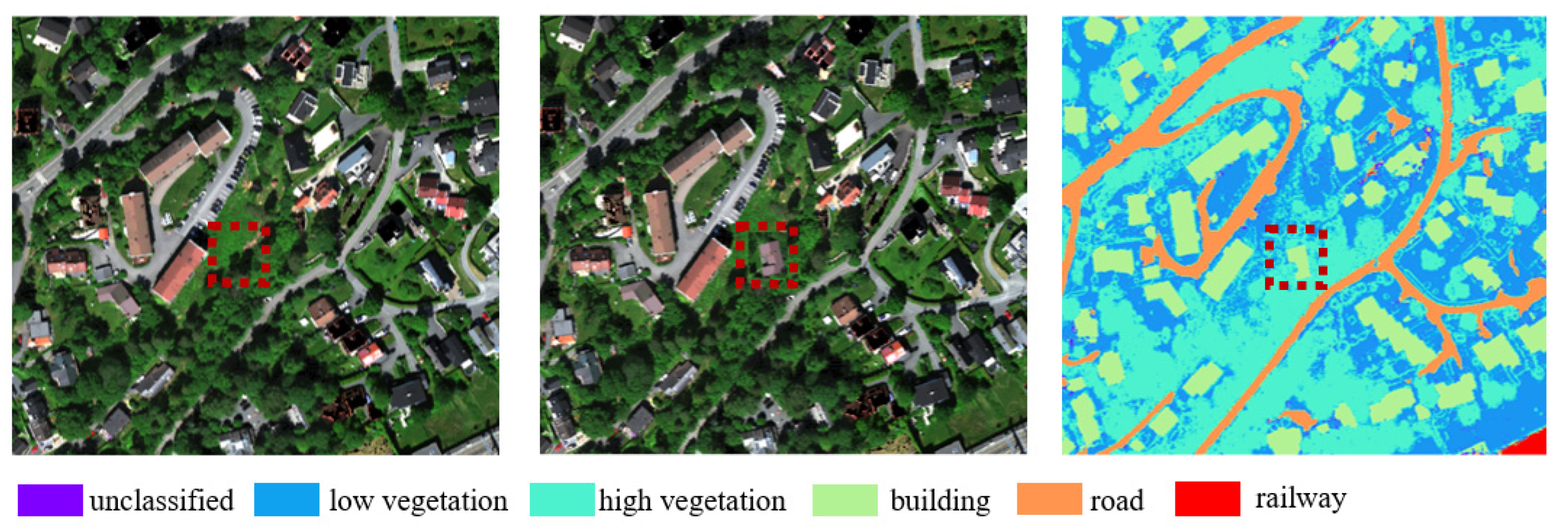
In order to diversify the analysis and prove the proposed method’s stability and correctness, we created simulated changes, adding a building in place of low and high vegetation. Our study area represents low dynamics of change over a short period. Therefore, such data simulation adds a significant change to the dataset. We assumed that the manual addition of a building in this location is feasible and typical for urban/suburban areas where vegetation is removed to build new residential neighborhoods. This building was not annotated in the ground truth in training.

3. Proposed Method

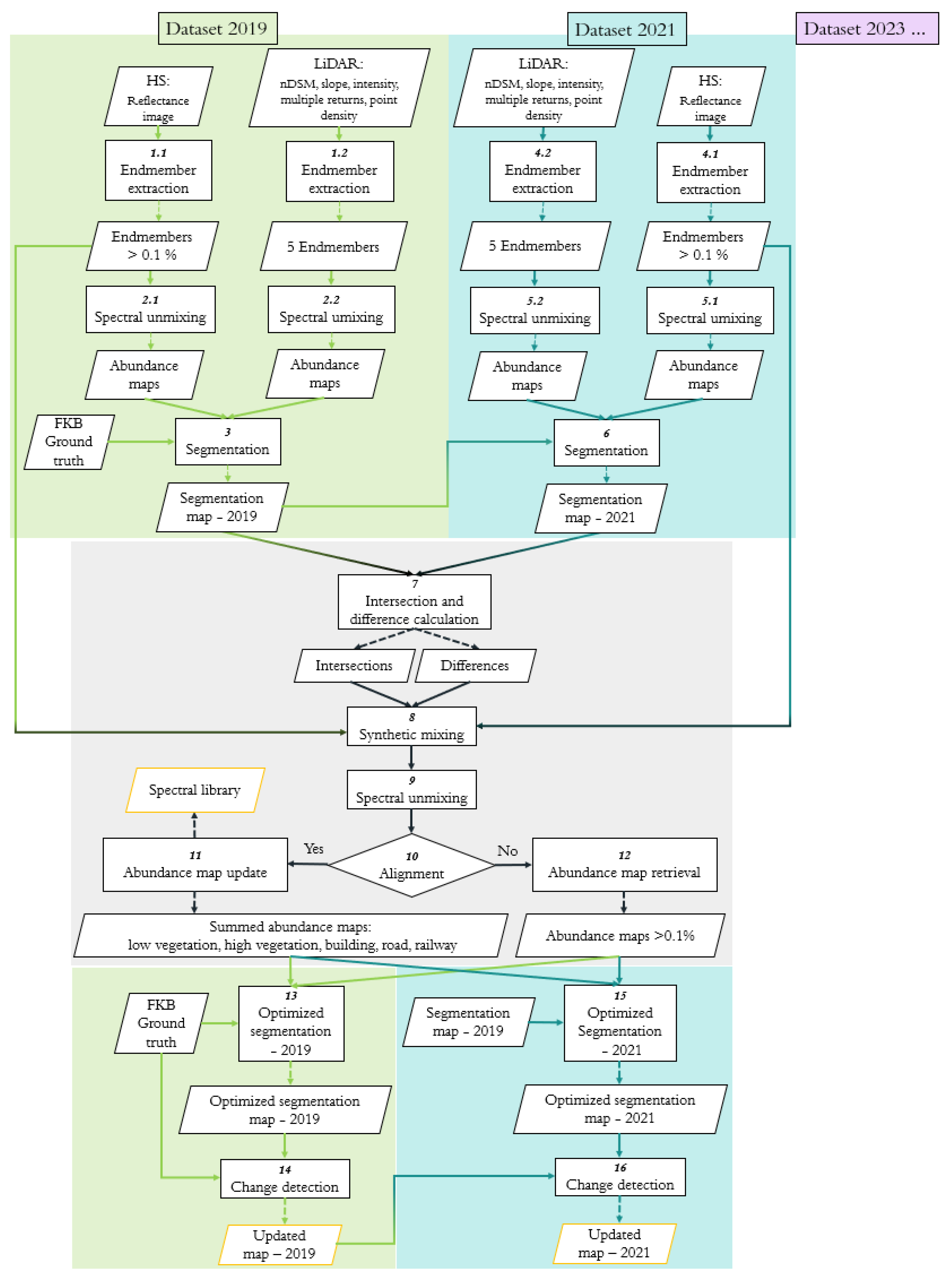
The following section describes an approach for multitemporal HL-Fusion at the feature level (Figure 2). Figure 2 represents a bitemporal problem with the possibility of adding new datasets to the approach. The analysis begins with unsupervised endmember extraction separately for the HS reflectance image (Figure 2, box 1.1) and five LiDAR features, such as nDSM, slope, intensity, multiple returns, and density (Figure 2, box 1.2) for the first time point (Figure 2, Dataset 2019). The number of endmembers created from HS data depends on the amount of each endmember in the scene and has been limited to all endmembers above 0.1 %. From the created endmembers, abundance maps are generated for HS (Figure 2, box 2.1) and LiDAR data (Figure 2, box 2.2), unmixing all endmembers spectrally and retrieving the percentage of each endmember per pixel in the scene. These abundance maps and the FKB ground truth data are fed into a segmentation algorithm (Figure 2, box 3). Then, analogous to the first dataset, the second time point (Figure 2, Dataset 2021) is analyzed, starting from endmember extraction to generation of abundance maps for HS (Figure 2, box 4.1 and 5.1) and LiDAR data (Figure 2, box 4.2 and 5.2). Then, the segmentation result from 2019, considered as the ground truth, is added to the segmentation for 2021 (Figure 2, box 6) along with retrieved abundance maps. From the segmentation results–segmentation maps from 2019 and 2021, segments are extracted for each defined class, calculating segment intersections and differences of datasets 2019 and 2021 (Figure 2, box 7). The most representative endmembers are extracted from each intersection and difference segments for the classes, such as low and high vegetation, building, road, and railway. In case endmembers from the difference group belong to one of the five predefined classes, synthetic mixing is applied (Figure 2, box 8). Then, spectral unmixing is carried out (Figure 2, box 9) to effectively and automatically align endmembers (Figure 2, box 10) from the existing difference group to the corresponding class and to update initial endmembers extracted before the first segmentation. From the updated endmembers, abundance maps are generated and summed for each defined class (Figure 2, box 11). The successful alignment is considered a basis for the automatic generation of a stable local spectral library with intraclass variability. The difference endmembers that cannot be aligned to any defined class were individually used for abundance map retrieval (Figure 2, box 12). All retrieved abundance maps are fed into the next iteration as optimized segmentation without parameter regularizations for 2019 (Figure 2, box 13) and 2021 datasets (Figure 2, box 15). The final step of the multitemporal analysis is change detection (Figure 2, box 14), where the original map to be updated (FKB ground truth) is compared with the segmentation results from the 2019 dataset, creating an updated map, which also shows the changes that have occurred in each of the five predefined classes. Analogously, the change detection (Figure 2, box 16) can be applied to dataset 2021, comparing the final map from dataset 2019 to the segmentation results from dataset 2021 and generating an updated map.

3.1. Endmember Extraction and Abundance Maps

In our study, we implemented the state-of-the-art iterative endmember extraction (EA) algorithm N-FINDR [51] for HS and LiDAR data, respectively (Figure 2, box 1.1, 1.2). We generated normalized abundance maps based on the extracted endmembers (Figure 2, box 2.1, 2.2) by applying the non-negativity-constrained least squares algorithm [58]. For HS EA, the preprocessed reflectance image was used to retrieve the most representative endmembers. For EA of LiDAR data, we built a LiDAR feature space where the five most relevant raster-based features have been extracted, including slope, the intensity from the first return, multiple returns, normalized digital surface model (nDSM), and point density. All the features were normalized separately before EA due to significant differences in the value scale.
The initially extracted endmembers for LiDAR data were used to generate abundance maps for each endmember, analogously to HS data.

3.2. Semantic Segmentation

The final input to semantic segmentation algorithms consists of abundance maps from HS and LiDAR data. We considered the 2D ResU-Net model architectures in this study [35,53,54], comparing the segmentation process with and without training data augmentation for 2019 (Figure 2, box 3) and 2021 (Figure 2, box 6) datasets without model parameter regularizations. The original U-Net consists of an encoder part with multiple blocks of convolutions and max pools for feature extraction and a corresponding decoder with transposed convolutions for upscaling after each convolution block [59]. Skip connections between corresponding convolution blocks in the encoder and decoder are used for improved class location and signal propagation. The Residual U-Net extends the original U-Net with local skip connections in the convolution blocks, further enhancing signal pathways and granularity of predictions. In the ResU-Net model, we implemented 2D convolutional operations, which are sufficient and not time-consuming in this type of land cover analysis [35].
The 2D ResU-Net models were implemented in Python using the module Tensorflow with GPU functionalities [60].

3.2.1. Implementation Details

For the segmentation, the study dataset was divided into 64 × 64 pixel patches, of which 70% is training, and 30% is the test dataset. A total of 20% of the training data is used for validation. Training, validation, and testing were selected, considering all classes equally in training, validation, and testing. In addition, data augmentation was applied to training data by applying a 50% overlap of each patch (Figure 3), of which no patch in the training dataset was part of the test dataset.

3.2.2. Evaluation Metrics

For segmentation purposes, we used standard metrics for measuring accuracy, applying F-Measure (F1 score) [61] and Matthews Correlation Coefficient (MCC). The F1 score is commonly used to accurately evaluate the boundaries in the predicted pixels [62]. The F1 score was applied for the overall algorithm performance assessment. The metrics take into account precision (p) and recall (r) in the predictions and are defined as follows:
p = T P T P + F P ,
r = T P T P + F N ,
and
F 1 s c o r e = 2 p r p + r
where true positives are defined as TP, false positives as FP, and false negatives as FN. The MCC is used for the accuracy evaluation of each class individually, suitable for data with imbalanced classes with the following formula:
M C C = ( T P T N ) ( F P F N ) ( T P + F P ) ( T P + F N ) ( T N + F P ) ( T N + F N ) ,
where true negatives are defined as TN. The MCC scales from −1 to 1, where −1 means that all predictions are incorrect and where 1, in contrast, predicted all results right [63].

3.2.3. Multitemporal Analysis—Intersection and Differences

Given that the semantic segmentation is conducted for all available datasets X at time X1, …, Xn for classes C1, …, Ci, each estimated segment of a single class from C1, …, Ci is handled individually (Figure 2, box 7).
For each class C1, …, Ci, common areas occurring in all datasets from different times X1, …, Xn are grouped into «intersection». It means that a pixel classified as class C1 (e.g., high vegetation) in all datasets X1, …, Xn (e.g., 2019 and 2021) is assigned to the intersection group. For each intersection of a class C1, …, Ci, we extracted representative endmembers from all datasets X1, …, Xn.
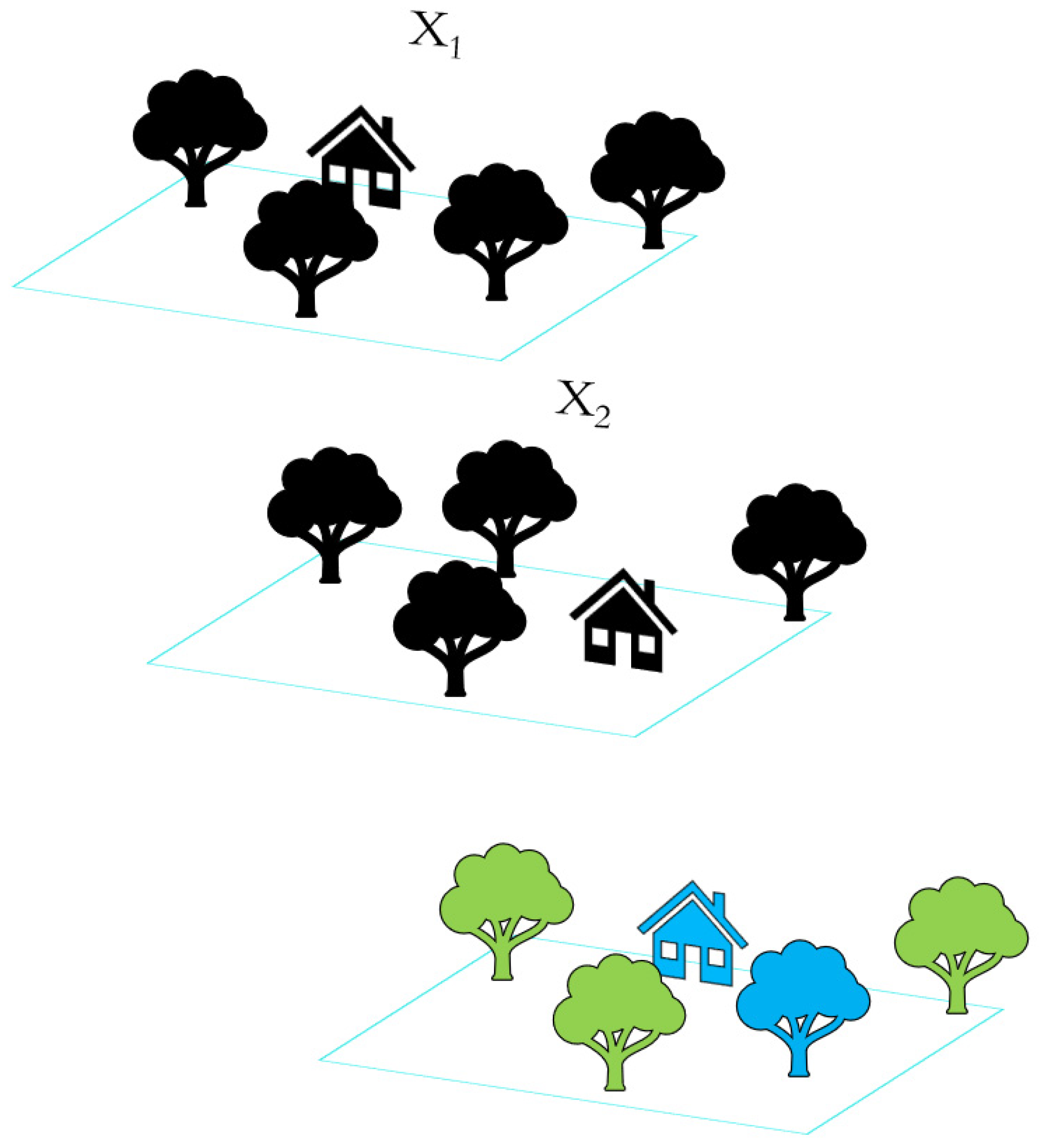
In contrast to an intersection, «difference» means that a pixel in dataset X1 was assigned to another class C than in dataset(s) X2, …, Xn. For each such difference of each class C1, …, Ci, we found representative endmembers and collected them in one difference group. Figure 4 represents two datasets, X1 and X2, where some trees (green color) correspond to the intersection group, and one house and one tree from dataset X1 (blue color) were not found in dataset X2 and therefore corresponded to the difference group.

3.3. Synthetic Mixing for Spectral Library Generation

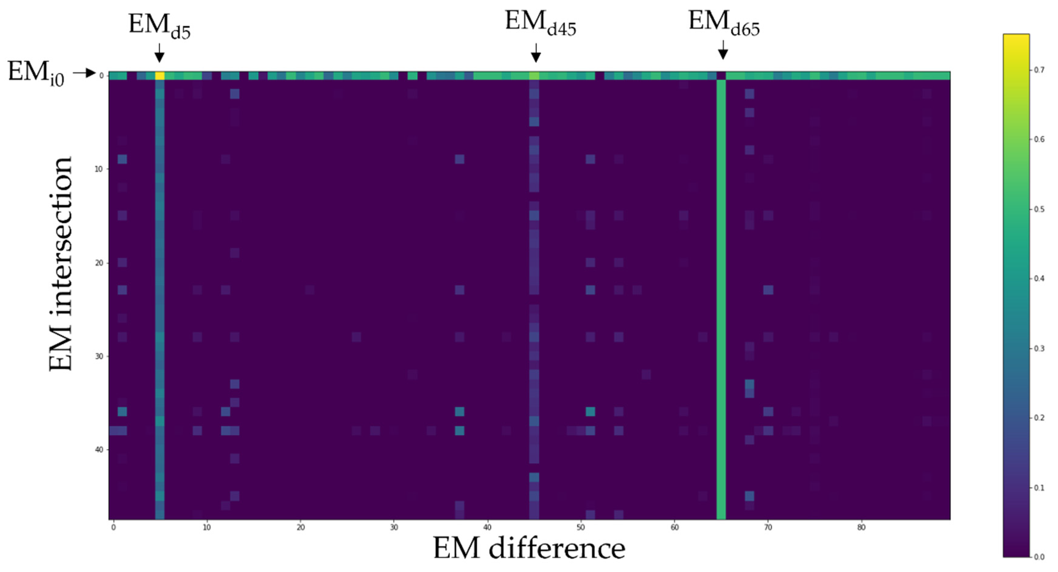
We assume some endmembers from the difference group can be assigned to any defined classes C1, …, Ci. Therefore, we synthetically mixed all intersection endmembers EMi0, …, EMin with all difference endmembers EMd0, …, EMdm, and initial endmembers generated for the first segmentation in proportion 50:50 percent (Figure 2, box 8). After the synthetic mixing, we unmixed the new synthetic matrix spectrally (Figure 2, box 9, Figure 5).
The intuition behind the spectral unmixing in this study is to align difference and initial endmembers to any of the defined classes C1, … Ci, comparing all difference and initial endmembers to all intersection endmembers (Figure 2, box 10). Figure 5 presents a spectral unmixing example, where each class C1, …, Ci consists of ten intersection endmembers (Table 1).
Given that the intersection endmember EMi0 belongs to the road class, we are searching for difference and initial endmembers with a similar unmixing value to EMi0. In this example, two difference endmembers, EMd5 and EMd65, are similar to EMi0 and were aligned automatically to the road class as the EMi0. For the updated intersection endmembers, abundance maps have been retrieved and summed up for each class separately (Figure 2, box 11). Such optimized intersection endmembers are the basis for a stable local spectral library.
The difference endmembers that were not aligned automatically to any defined classes were used to retrieve abundance maps for the second segmentation iteration (Figure 2, box 12). However, to avoid noise and endmembers that are not substantial, we calculated the average of each difference endmember occurring in our study area and limited the amount of the endmembers contributing with a value above 0.1%. The updated intersection abundance maps, difference abundance maps, and LiDAR features extracted for the first segmentation were merged and fed as input for the second segmentation iteration for the 2019 (Figure 2, box 13) and 2021 (Figure 2, box 15) datasets.

3.4. Change Detection

In order to update the local map that served as the ground truth (FKB) for segmentation for the 2019 dataset, we subtracted each segment separately from the 2019 dataset from the FKB reference data highlighting land cover changes (Figure 2, box 14). The resulting update map indicates the changes in objects/surfaces added or removed in 2019. This procedure was analogously repeated for change detection (Figure 2, box 16) for retrieving an updated map for the 2019 to 2021 dataset. (Figure 4, box 18). Since there were no significant changes in the defined classes in artificial objects such as buildings and railways from 2019 to 2021, we simulated a change and added a random building in place of low/high vegetation in the dataset from 2021.

4. Experimental Results

This section provides results for the initial (first iteration) and optimized the second iteration (after the abundance map update) segmentation task for 2D ResU-Net with and without data augmentation for 2019 and 2021 datasets. The results of the spectral library generated from the best segmentation results of 2019 and 2021 are presented. Then, the results of the change simulation are shown, as well as the results of the change detection for each of the defined classes taking into account the changes from the FKB reference data for 2019 and from 2019 to 2021.

4.1. Segmentation Results

Figure 6 shows the HS scenes from the datasets from 2019 (a) and 2021 (c) with corresponding ground truths for 2019 (c) and 2021 (d).
Table 2 presents the segmentation results for 2019 and 2021 of the ResU-Net without data augmentation for initial segmentation (segmentation I) and optimized segmentation (segmentation II). The results are based on MCC for each class and the F1 score metric for overall segmentation. Corresponding segmentation maps are shown in Figure 7.
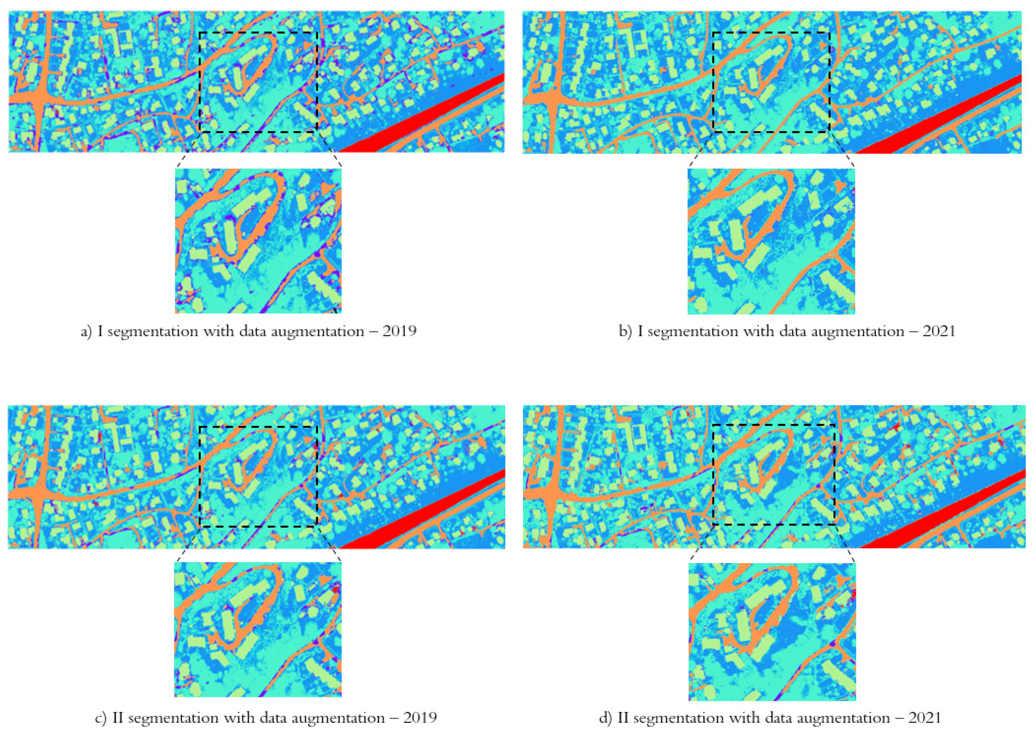
Similarly, the results for segmentation with data augmentation are reported in Table 3 and Figure 8 for the 2019 and 2021 datasets. The results from Table 2 and Table 3 show that, regardless of the data augmentation process, the accuracy based on MCC increases for both individual classes and the overall F1 score after the second iteration of the segmentation. Comparing the results of segmentation without and with data augmentation, the segmentation with data augmentation achieves higher results in both initial (I) and optimized (II) segmentation.

4.2. Spectral Library

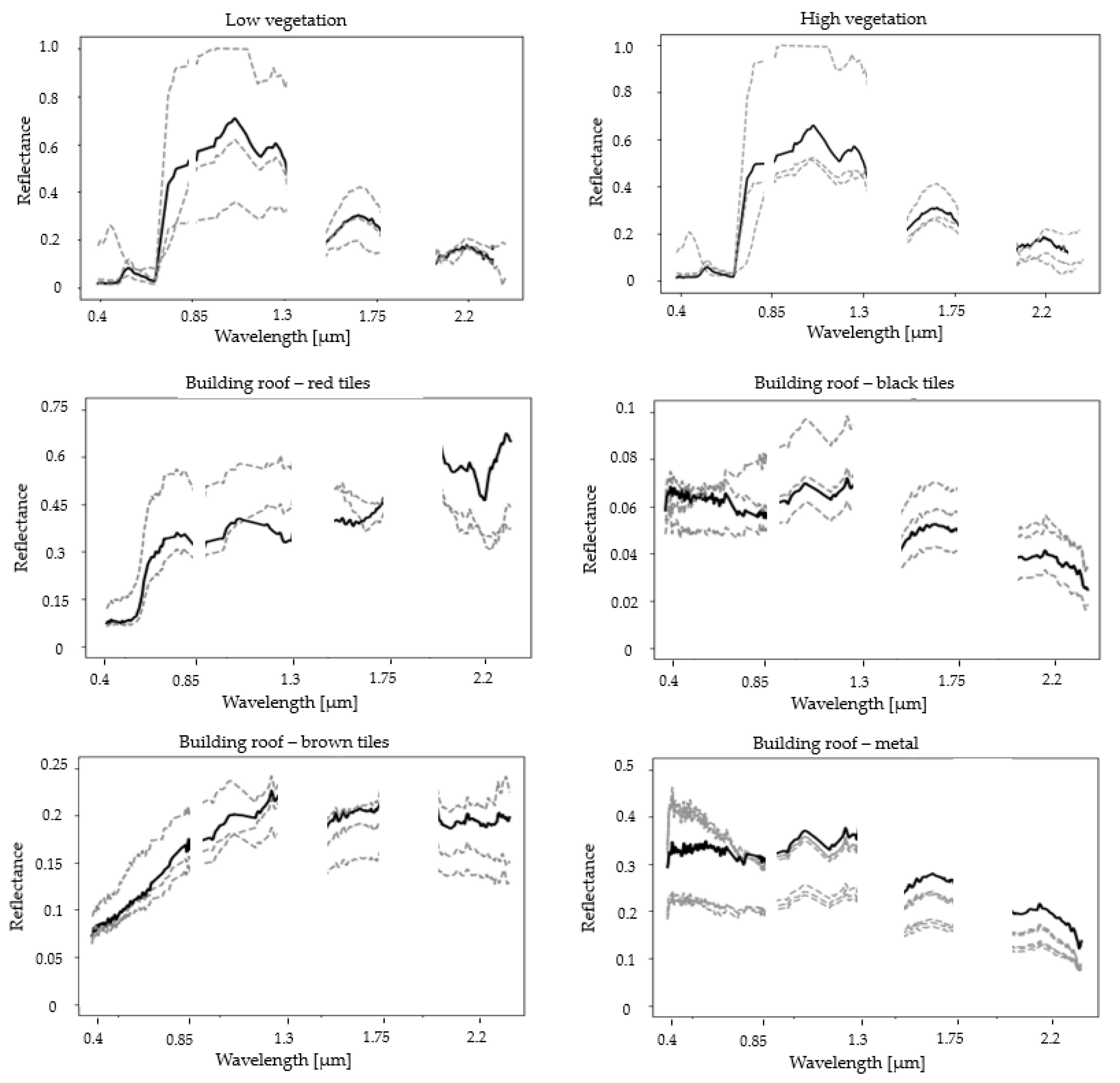
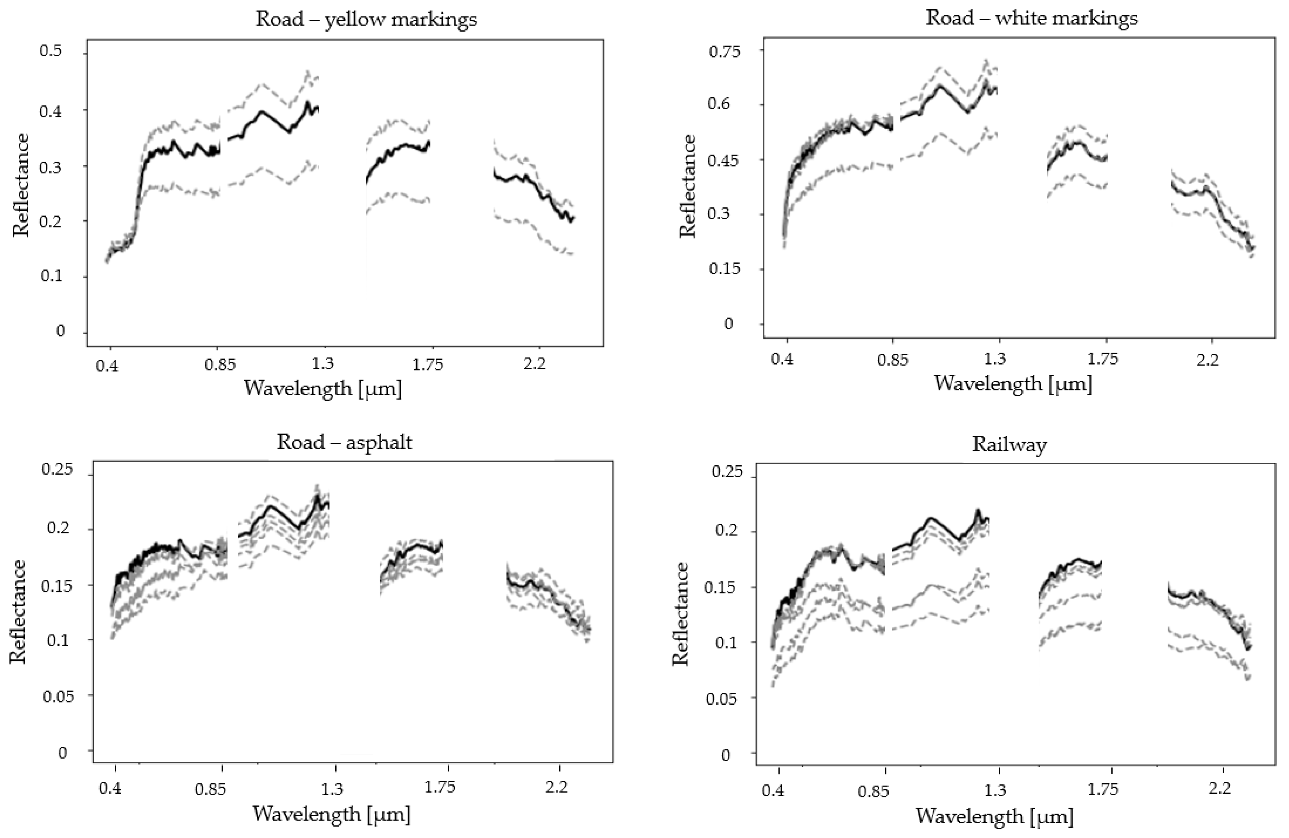
The spectral library was generated based on the results of the initial (I) segmentation of 2019 and 2021 and then updated after the results of the optimized (II) segmentation. The spectral library, shown in Figure 9, demonstrated the final spectra for each class, including low and high vegetation, buildings, roads, and railways. Each spectrum covers the 0.4−2.35 µm spectral range. Noisy bands from the preprocessing are not included either in the analysis or in the built spectral library. Each class contains the most representative spectra within its definition, i.e., the building class consists of different roof materials depending on their complexity and heterogeneity in the selected study of interest. We have selected red, black, and brown tiles and metal roofing.

4.3. Change Detection

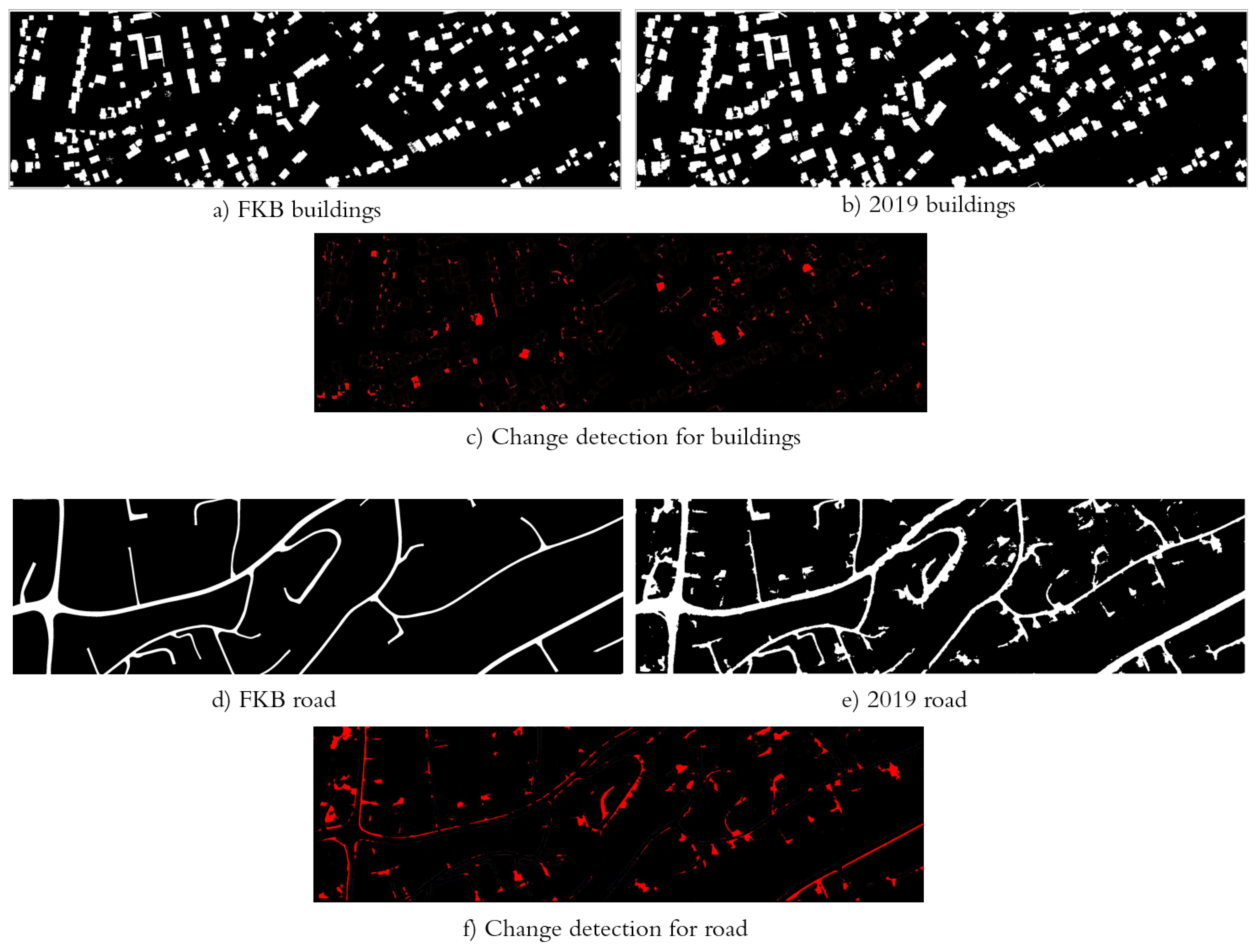
Figure 10 demonstrates the change detection results for the changes from the FKB reference data to 2019 for buildings and roads. The railway class has not experienced changes.
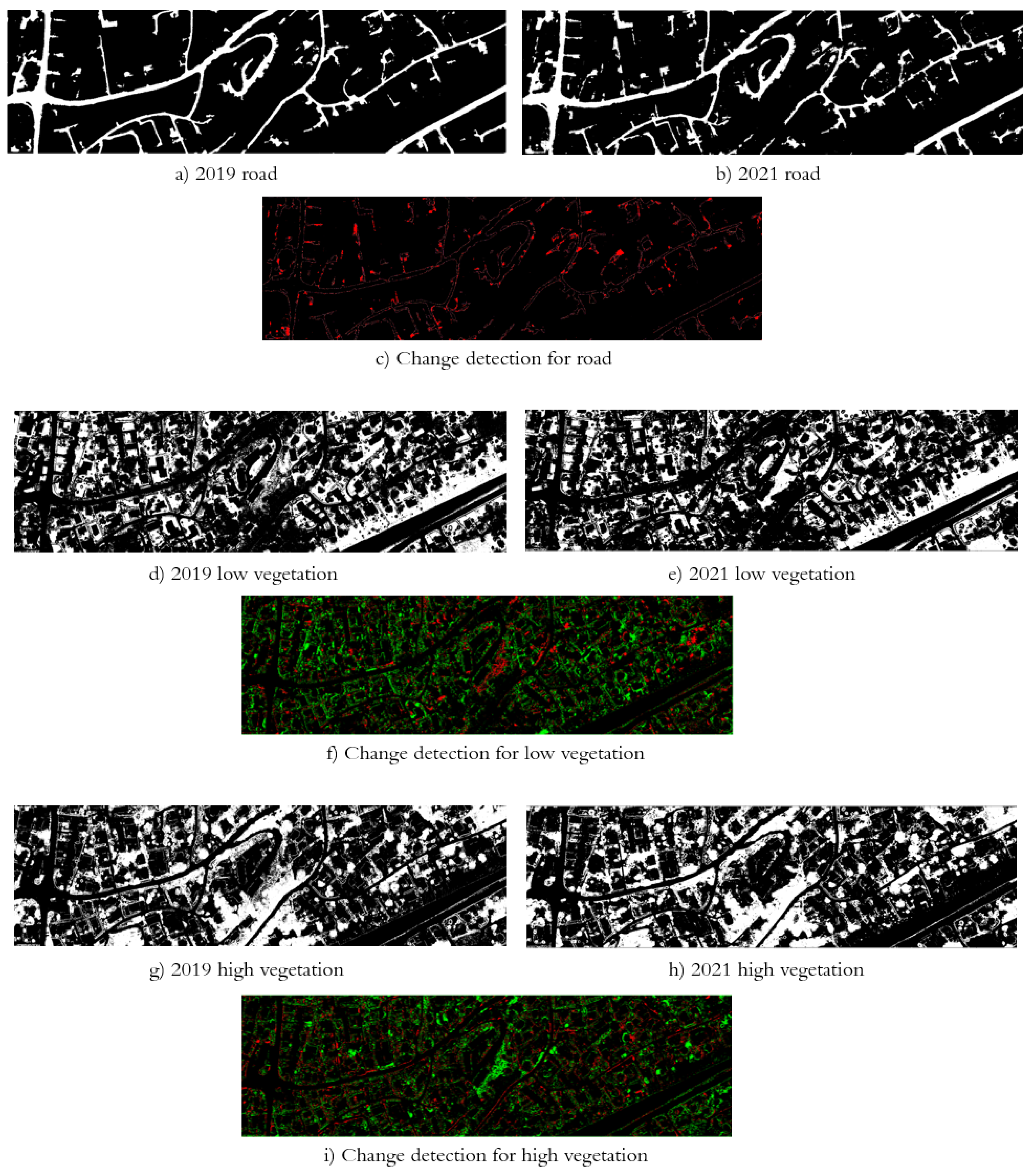
Figure 11 depicts the change detection results from 2019 to 2021 for roads, low and high vegetation.
Table 4 presents the MCC accuracy results for segmentation on a dataset where a building was added in the 2021 dataset. Figure 12 highlights the simulated building addition with the building found in the segmentation process.

5. Discussion

5.1. Segmentation Process

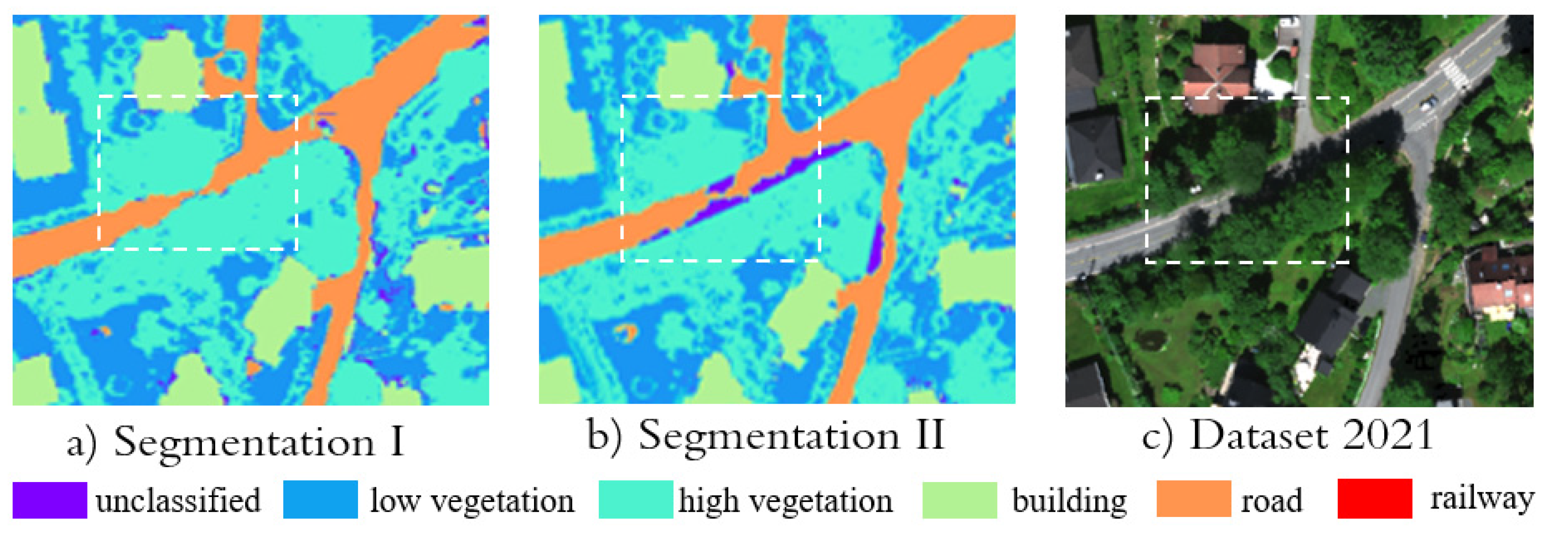
In the segmentation of high-dimensional data, dimension reduction is crucial [64]. Unsupervised endmember extraction and retrieval of abundance maps provide a stable and reliable method for obtaining the most representative features of a scene that are not calculated based on statistics. Based on the segmentation results from 2019 and 2021, it has to be noted that only in single classes, such as railway in 2021, the second iteration of segmentation after optimization deteriorated accuracy from 99 to 98%. Comparing all classes in general, low and high vegetation achieved significantly lower accuracy than the buildings, roads, and railways. This is because ground truth data for these classes were created semi-automatically, which is insufficiently accurate. In addition, in many places in our study area, vegetation partially covers some objects, such as roads and buildings, depending on the season in which the data acquisition campaign was carried out. For this reason, some road pixels were not found in the segmentation. The main aspect is that HS data do not penetrate the surface, and some extracted features from LiDAR, such as intensity, include information from the surface only, i.e., from the first laser return. Figure 13 shows an example of high vegetation covering a road.
In the I segmentation (Figure 13a), vegetation was identified on the road, degrading the road accuracy results. In the II segmentation, vegetation covering the road was reclassified to the unknown class. When a classification of new objects or surfaces is required, one of the new classes in this study of interest could be "vegetation on the road" [65]. Such information about vegetation covering main roads can be an indicator for municipalities to remove and secure high vegetation that threatens vehicular traffic and is a typical highlight of urban complexity.
In addition to the improved accuracy of the results in the second iteration of segmentation, after segmentation optimization, in most objects, the edges have been sharpened, and the geometry in the 2D plane is approximated to reality. This is especially noticeable in objects not marked in ground truth data but present in the analyzed dataset, such as building detection in Figure 14.
A frequent challenge in multiclass segmentation using 2D convolutional operations is patch edge effects. These effects relate to the generation of "contours" of each 64 × 64 pixel patch in the classification results, meaning that contextual information from neighboring pixels is not included at the pixel patch edges (Figure 7a). This unintentional effect has been reported in previous studies, where Kuras et al. [35] implemented 3D instead of 2D convolutional operations in the model, mitigating edge effects in the final segmentation map. However, in this study, 3D convolutions require increased computation time, especially when applying data augmentation. Initial experiments on 3D convolutional operations have been carried out, achieving similar results using much larger computational resources. Therefore, 2D convolutions are sufficient for this purpose, providing solid results [35].
In our study, the second iteration of the segmentation eliminates patch edge effects, thereby improving accuracy results (Figure 7c,d). On the other hand, data augmentation through a patch overlap of 50% in the training dataset not only levels edge effects in the I segmentation already (Figure 8a,c) but also allows for more stable learning of the algorithm of localization patterns helping in object identification.
Another important aspect worth discussing is achieving 100% accuracy in some classes. This is a sign of overfitting, which can be compensated for by reducing the complexity of the segmentation model. The splitting of training may have caused overfitting, and test data was carried out patch-wise rather than strictly object-wise, causing the same object/surface to occur both in training and test data. Also, the weight of each class may have been disproportionate, with the rest getting more focus in the segmentation. However, to prevent overfitting issues, the early stopping function was used to save training time and stop training when the model achieved the best performance.

5.2. Spectral Library

Since the defined classes in the segmentation in the urban environment are complex and heterogeneous, the automatically created spectral library for each class contains spectra belonging to different materials and surfaces within that class. One example is the road class which consists of not only the primary road material—asphalt or concrete, but also road surface markings which, due to the spatial resolution of 0.3 m, are mixed with the asphalt or the vehicle on the street. Figure 9 shows that some spectra, especially in low and high vegetation, experience saturation caused by technical problems in data acquisition or atmospheric correction. Errors and artifacts in the spectral library can also be caused by the level adjustment between VNIR and SWIR sensors and the fact that these two cameras do not point to the same spot from the airplane, which is particularly problematic when dealing with a dynamic environment where, for example, vehicles are constantly moving. With the insertion of new datasets into the analysis, i.e., temporal or spatial, new material/spectra may appear that do not belong to the five classes defined in this approach. In case a new class arises, it can be easily added to the collection in the spectral library and defined the class manually if applicable considering available spectral libraries [66,67]. Such a spectral library can be used for plausibility checking and refining the classification. Overlap between classes, such as vegetation on the house roof, indicates overgrowth of trees, meadow, or moos roof. Depending on the application and purpose, this complexity can be explored, defined, and controlled using the spectral library.

5.3. Change Detection

Change detection for all defined classes is shown in Figure 10 and 11. The most significant changes could be experienced when the updated map represented 2019. In 2019, several new buildings were detected and updated. Sometimes in building maps, we notice detected changes with already known buildings. This is because boats and cars on the properties were assigned to the building class. In the case of road change detection, as roads were defined, property entrances or alleys were not marked in the original reference data. In addition, the algorithm also detected changes when ground truth was prepared manually, and the object from the airborne-based image perspective slightly shifted or changed object edges. However, erroneous labeling can result in lowered accuracy values. It is, therefore, crucial that labeling of ground truths is only performed where one is entirely confident of the correctness.
Furthermore, it is crucial to point out that our novel framework has effectively identified actual or simulated objects and when ground truth data are not aligned with the current position, as is the case with local map updates.
Our framework allows the addition of new time point datasets, thanks to which the focus of the analysis can be on high-frequent and low-frequent changes or mobile and static object recognition in an urban scene. Moreover, adding another dataset allows for building a stable spectral library and features that can be transferred to other study areas. Objects and surfaces not identified during segmentation can be manually added, allowing for dynamic class extension of urban land cover.
However, it is important to mention that the scene chosen for this study was slightly distant from the city center. This project will likely prove more complicated if a more complex and heterogeneous scene is selected.

6. Conclusions

This study presents a novel approach to feature-level-based multisensor data fusion of HS and LiDAR data proposing a method for an effective segmentation optimization based on the unsupervised endmember extraction and abundance map retrieval of HS and LiDAR data without parameter regularizations. Objects and materials that have not been identified can be added manually, with the possibility of dynamic expansion and various land cover classes. All the models achieved increased segmentation results after segmentation optimization, regardless of applying data augmentation. The ResU-Net with implemented data augmentation outperformed compared to models without data augmentation, helping the model learn contextual information about the object. In addition, a local spectral library has been generated automatically as a by-product that can be used to expand the local urban database and serve as a basis for further updates of this region. Based on the segmentation and generated spectral library, we created a change map of each defined class, creating a local map update.

7. Future Work

Our novel approach serves as a promising basis for developing a change detection framework based on unsupervised segmentation for multitemporal data from multiple sensors. Such unsupervised segmentation would limit issues related to the preparation of the ground truth data, which are not always available and updated for the algorithm to learn correctly segment complex objects and surfaces. The proposed framework of change detection applying fused HS and LiDAR data at the feature level can be expanded with more datasets of the study area, allowing segmentation and spectral signatures of individual objects or surfaces to be more stable and reliable in defining new objects in more complex urban scenes.

Author Contributions

Conceptualization, A.K. and M.B.; analysis, A.K.; investigation, A.K.; writing—original draft preparation, A.K.; writing—review and editing, M.B., K.H.L. and I.B.; visualization, A.K.; supervision, I.B. All authors have read and agreed to the published version of the manuscript.

Funding

This work is part of the project “FKB maskinlæring” funded by RFF “Oslo og Akershus Regionale forskningsfond” (295836).

Data Availability Statement

Not applicable.

Acknowledgments

The authors acknowledge the Orion High Performance Computing Center (OHPCC) at the Norwegian University of Life Sciences (NMBU) for providing computational resources that have contributed to the research results reported within this paper. URL (internal): https://orion.nmbu.no, accessed 10 December 2022. The authors thank Vetle Jonassen from Field Group AS for providing the data and support.

Conflicts of Interest

The authors declare no conflict of interest. The funders had no role in the design of the study; in the collection, analyses, or interpretation of data; in the writing of the manuscript; or in the decision to publish the results.

References

  1. Heiden, U.; Segl, K.; Roessner, S.; Kaufmann, H. Determination of robust spectral features for identification of urban surface materials in hyperspectral remote sensing data. Remote Sens. Environ. 2007, 111, 537–552. [Google Scholar] [CrossRef] [Green Version]
  2. Cadenasso, M.L.; Pickett, S.T.A.; Schwarz, K. Spatial heterogeneity in urban ecosystems: Reconceptualizing land cover and a framework for classification. Front. Ecol. Environ. 2007, 5, 80–88. [Google Scholar] [CrossRef]
  3. Jing, C.; Zhou, W.; Qian, Y.; Yu, W.; Zheng, Z. A novel approach for quantifying high-frequency urban land cover changes at the block level with scarce clear-sky Landsat observations. Remote Sens. Environ. 2021, 255, 112293. [Google Scholar] [CrossRef]
  4. Banzhaf, E.; Kabisch, S.; Knapp, S.; Rink, D.; Wolff, M.; Kindler, A. Integrated research on land-use changes in the face of urban transformations—An analytic framework for further studies. Land Use Policy 2017, 60, 403–407. [Google Scholar] [CrossRef]
  5. Hegazy, I.R.; Kaloop, M.R. Monitoring urban growth and land use change detection with GIS and remote sensing techniques in Daqahlia governorate Egypt. Int. J. Sustain. Built Environ. 2015, 4, 117–124. [Google Scholar] [CrossRef] [Green Version]
  6. Wellmann, T.; Lausch, A.; Andersson, E.; Knapp, S.; Cortinovis, C.; Jache, J.; Scheuer, S.; Kremer, P.; Mascarenhas, A.; Kraemer, R.; et al. Remote sensing in urban planning: Contributions towards ecologically sound policies? Landsc. Urban Plan. 2020, 204, 103921. [Google Scholar] [CrossRef]
  7. Yin, J.; Dong, J.; Hamm, N.A.S.; Li, Z.; Wang, J.; Xing, H.; Fu, P. Integrating remote sensing and geospatial big data for urban land use mapping: A review. Int. J. Appl. Earth Obs. Geoinf. 2021, 103, 102514. [Google Scholar] [CrossRef]
  8. Kuras, A.; Brell, M.; Rizzi, J.; Burud, I. Hyperspectral and Lidar Data Applied to the Urban Land Cover Machine Learning and Neural-Network-Based Classification: A Review. Remote Sens. 2021, 13, 3393. [Google Scholar] [CrossRef]
  9. Shahtahmassebi, A.R.; Li, C.; Fan, Y.; Wu, Y.; Iin, Y.; Gan, M.; Wang, K.; Malik, A.; Blackburn, G.A. Remote sensing of urban green spaces: A review. Urban For. Urban Green. 2021, 57, 126946. [Google Scholar] [CrossRef]
  10. Roessner, S.; Segl, K.; Heiden, U.; Kaufmann, H. Automated differentiation of urban surfaces based on airborne hyperspectral imagery. IEEE Trans. Geosci. Remote Sens. 2001, 39, 1525–1532. [Google Scholar] [CrossRef]
  11. Tan, K.; Wang, H.; Chen, L.; Du, Q.; Du, P.; Pan, C. Estimation of the spatial distribution of heavy metal in agricultural soils using airborne hyperspectral imaging and random forest. J. Hazard. Mater. 2020, 382, 120987. [Google Scholar] [CrossRef]
  12. Qu, J.; Hou, S.; Dong, W.; Li, Y.; Xie, W. A Multi-Level Encoder-Decoder Attention Network for Change Detection in Hyperspectral Images. IEEE Trans. Geosci. Remote Sens. 2021, 60, 5518113. [Google Scholar] [CrossRef]
  13. Campbell, J.B. Introduction to Remote Sensing; Guilford Press: New York, NY, USA, 2010. [Google Scholar]
  14. Song, A.; Choi, J.; Han, Y.; Kim, Y. Change Detection in Hyperspectral Images Using Recurrent 3D Fully Convolutional Networks. Remote Sens. 2018, 10, 1827. [Google Scholar] [CrossRef] [Green Version]
  15. Bruzzone, L.; Bovolo, F. A Novel Framework for the Design of Change-Detection Systems for Very-High-Resolution Remote Sensing Images. Proc. IEEE 2012, 101, 609–630. [Google Scholar] [CrossRef]
  16. Aksoy, S. Spatial techniques for image classification. In Signal and Image Processing for Remote Sensing; CRC Press: Boca Raton, FL, USA, 2008; pp. 491–513. [Google Scholar]
  17. Benediktsson, J.A.; Palmason, J.A.; Sveinsson, J.R. Classification of hyperspectral data from urban areas based on extended morphological profiles. IEEE Trans. Geosci. Remote Sens. 2005, 43, 480–491. [Google Scholar] [CrossRef]
  18. Jouni, M.; Mura, M.D.; Comon, P. Hyperspectral Image Classification Based on Mathematical Morphology and Tensor Decomposition. Math. Morphol. Theory Appl. 2020, 4, 1–30. [Google Scholar] [CrossRef] [Green Version]
  19. Mura, M.D.; Benediktsson, J.A.; Waske, B.; Bruzzone, L. Extended profiles with morphological attribute filters for the analysis of hyperspectral data. Int. J. Remote Sens. 2010, 31, 5975–5991. [Google Scholar] [CrossRef]
  20. Bovolo, F. A Multilevel Parcel-Based Approach to Change Detection in Very High Resolution Multitemporal Images. IEEE Geosci. Remote Sens. Lett. 2008, 6, 33–37. [Google Scholar] [CrossRef] [Green Version]
  21. Plaza, A.; Benediktsson, J.A.; Boardman, J.W.; Brazile, J.; Bruzzone, L.; Camps-Valls, G.; Chanussot, J.; Fauvel, M.; Gamba, P.; Gualtieri, A.; et al. Recent advances in techniques for hyperspectral image processing. Remote Sens. Environ. 2009, 13, 110–122. [Google Scholar] [CrossRef]
  22. Sun, L.; Wu, Z.; Liu, J.; Xiao, L.; Wei, Z. Supervised spectral-spatial hyperspectral image classification with weighted Markov Random Fields. IEEE Trans. Geosci. Remote Sens. 2015, 53, 1490–1503. [Google Scholar] [CrossRef]
  23. Li, J.; Bioucas-Dias, J.M.; Plaza, A. Spectral-spatial hyperspectral image segmentation using subspace multinomial logistic regression and markov random fields. IEEE Trans. Geosci. Remote Sens. 2012, 50, 809–823. [Google Scholar] [CrossRef]
  24. Cao, X.; Zhou, F.; Xu, L.; Meng, D.; Xu, Z.; Paisley, J. Hyperspectral image classification with markov random fields and a convolutional neural network. IEEE Trans. Image Process. 2017, 27, 2354–2367. [Google Scholar] [CrossRef] [PubMed] [Green Version]
  25. Li, Y.; Zhang, H.; Shen, Q. Spectral–spatial classification of hyperspectral imagery with 3D convolutional neural network. Remote Sens. 2017, 9, 67. [Google Scholar] [CrossRef] [Green Version]
  26. Alonzo, M.; Bookhagen, B.; Roberts, D.A. Urban tree species mapping using hyperspectral and lidar data fusion. Remote Sens. Environ. 2014, 148, 70–83. [Google Scholar] [CrossRef]
  27. Zhao, X.; Tao, R.; Li, W.; Li, H.C.; Du, Q.; Liao, W.; Philips, W. Joint Classification of Hyperspectral and LiDAR Data Using Hierarchical Random Walk and Deep CNN Architecture. IEEE Trans. Geosci. Remote Sens. 2020, 58, 7355–7370. [Google Scholar] [CrossRef]
  28. Hong, D.; Gao, L.; Hang, R.; Zhang, B.; Chanussot, J. Deep encoder-decoder networks for classification of hyperspectral and LiDAR data. IEEE Geosci. Remote Sens. Lett. 2020, 99, 1–5. [Google Scholar] [CrossRef]
  29. Feng, Q.; Zhu, D.; Yang, J.; Li, B. Multisource Hyperspectral and LiDAR Data Fusion for Urban Land-Use Mapping based on a Modified Two-Branch Convolutional Neural Network. ISPRS Int. J. Geoinf. 2019, 8, 28. [Google Scholar] [CrossRef] [Green Version]
  30. Fang, L.; Zhu, D.; Yue, J.; Zhang, B.; He, M. Geometric-Spectral Reconstruction Learning for Multi-Source Open-Set Classification With Hyperspectral and LiDAR Data. IEEE/CAA J. Automat. Sin. 2022, 9, 1892–1895. [Google Scholar] [CrossRef]
  31. Gaulton, R.; Malthus, T.J. LiDAR mapping of canopy gaps in continuous cover forests: A comparison of canopy height model and point cloud based techniques. Int. J. Remote Sens. 2008, 31, 17–19. [Google Scholar] [CrossRef]
  32. Morsdorf, F.; Meier, E.; Allgöwer, B.; Nüesch, D. Clustering in airborne laser scanning raw data for segmentation of single trees. Int. Arch. Photogramm. Remote Sens. Spat. Inform. Sci. 2003, 34, W13. [Google Scholar]
  33. Marinelli, D.; Paris, C.; Bruzzone, L. An Approach to Tree Detection Based on the Fusion of Multitemporal LiDAR Data. IEEE Geosci. Remote Sens. Lett. 2019, 99, 1–5. [Google Scholar] [CrossRef]
  34. Yu, H.; Lu, X.; Cheng, G.; Ge, X. Detection and volume estimation of mining subsidence based on multi-temporal LiDAR data. In Proceedings of the 19th International Conference on Geoinformatics, Shanghai, China, 24–26 June 2011. [Google Scholar]
  35. Kuras, A.; Jenul, A.; Brell, M.; Burud, I. Comparison of 2D and 3D semantic segmentation in urban areas using fused hyperspectral and lidar data. J. Spectr. Imag. 2022, 11, a11. [Google Scholar] [CrossRef]
  36. Senchuri, R.; Kuras, A.; Burud, I. Machine Learning Methods for Road Edge Detection on Fused Airborne Hyperspectral and LIDAR Data. In Proceedings of the 11th Workshop on Hyperspectral Imaging and Signal Processing: Evolution in Remote Sensing (WHISPERS), Amsterdam, Netherlands, 24–26 March 2021. [Google Scholar]
  37. Singh, M.K.K.; Mohan, S.; Kumar, B. Fusion of hyperspectral and LiDAR data using sparse stacked autoencoder for land cover classification with 3D-2D convolutional neural network. J. Appl. Remote Sens. 2022, 16, 034523. [Google Scholar] [CrossRef]
  38. Degerickx, J.; Roberts, D.A.; McFadden, J.P.; Hermy, M.; Somers, B. Urban tree health assessment using airborne hyperspectral and LiDAR imagery. Int. J. Appl. Earth Obs. Geoinf. 2018, 73, 26–38. [Google Scholar] [CrossRef] [Green Version]
  39. Hänsch, R.; Hellwich, O. Fusion of Multispectral LiDAR, Hyperspectral and RGB Data for Urban Land Cover Classification. IEEE Geosci. Remote Sens. Lett. 2021, 18, 366–370. [Google Scholar] [CrossRef]
  40. Brell, M.; Segl, K.; Guanter, L.; Bookhagen, B. Hyperspectral and Lidar Intensity Data Fusion: A Framework for the Rigorous Correction of Illumination, Anisotropic Effects, and Cross Calibration. IEEE Trans. Geosci. Remote Sens. 2017, 55. [Google Scholar] [CrossRef] [Green Version]
  41. Brell, M.; Segl, K.; Guanter, L.; Bookhagen, B. 3D hyperspectral point cloud generation: Fusing airborne laser scanning and hyperspectral imaging sensors for improved object-based information extraction. ISPRS J. Photogramm. Remote Sens. 2019, 149, 200–214. [Google Scholar] [CrossRef]
  42. Khaleghi, B.; Khamis, A.; Karray, F.; Razavi, S.N. Multisensor Data Fusion: A Review of the State-of-the-art. Inf. Fusion 2013, 14. [Google Scholar] [CrossRef]
  43. Kahramann, S.; Bacher, R. A comprehensive review of hyperspectral data fusion with lidar and sar data. Ann. Rev. Control 2021, 51, 236–253. [Google Scholar] [CrossRef]
  44. Voss, M.; Sugumaran, R. Seasonal Effect on Tree Species Classification in an Urban Environment Using Hyperspectral Data, LiDAR, and an Object- Oriented Approach. Sensors 2008, 8, 3020–3036. [Google Scholar] [CrossRef] [Green Version]
  45. Man, Q.; Dong, P.; Guo, H. Pixel- and feature-level fusion of hyperspectral and lidar data for urban land-use classification. Int. J. Remote Sens. 2015, 36, 1618–1644. [Google Scholar] [CrossRef]
  46. Ojala, T.; Pietikainen, M.; Maenpaa, T.T. Multi resolution gray scale and rotation invariant texture classification with local binary pattern. IEEE Trans. Pattern Anal. Mach. Intell. 2002, 24, 971–987. [Google Scholar] [CrossRef]
  47. Shirowzhan, S.; Trinder, J. Building classification from LiDAR data for spatial-temporal assessment of 3D urban developments. Proced. Eng. 2017, 180, 1453–1461. [Google Scholar] [CrossRef]
  48. Thenkabail, P.S.; Smith, R.B.; Pauw, E.D. Hyperspectral Vegetation Indices and Their Relationships with Agricultural Crop Characteristics. Remote Sens. Environ. 2000, 71, 158–182. [Google Scholar] [CrossRef]
  49. Hasani, H.; Samadzadegan, F.; Reinartz, P. A metaheuristic feautre-level fusion strategy in classification of urban area using hyperspectral imagery and LiDAR data. Eur. J. Remote Sens. 2017, 50, 222–236. [Google Scholar] [CrossRef] [Green Version]
  50. Khodadadzadeh, M.; Li, J.; Prasad, S.; Plaza, A. Fusion of Hyperspectral and LiDAR Remote Sensing Data Using Multiple Feature Learning. IEEE J. Sel. Top. Appl. Earth Obersvat. Remote Sens. 2015, 8, 2971–2983. [Google Scholar] [CrossRef]
  51. Winter, M.E. N-FINDR: An algorithm for fast autonomous spectral end-member determination in hyperspectral data. Imaging Spectroscopy V 1999, 3753, 266–275. [Google Scholar]
  52. LeCun, Y.; Bengio, Y.; Hinton, G. Deep learning. Nature 2015, 521, 436–444. [Google Scholar] [CrossRef]
  53. Yang, X.; Li, X.; Ye, Y.; Zhang, X.; Zhang, H.; Huang, X.; Zhang, B. Road detection via deep residual dense u-net. In Proceedings of the International Joint Conference on Neural Networks, Budapest, Hungary, 14–19 July 2019. [Google Scholar]
  54. Zhang, Z.; Liu, Q.; Wang, Y. Road extraction by deep residual u-net. IEEE Geosci. Remote Sens. Lett. 2018, 15. [Google Scholar] [CrossRef] [Green Version]
  55. Schläpfer, D.; Richter, R. Geo-atmospheric processing of airborne imaging spectrometry data. Part1: Parametric orthorectification. Int. J. Remote Sens. 2002, 23, 2609–2630. [Google Scholar] [CrossRef]
  56. Green, A.A.; Berman, M.; Switzer, P.; Craig, M.D. A transformation for ordering multispectral data in terms of image quality with implications for noise removal. IEEE Trans. Geosci. Remote Sens. 1988, 26, 65–74. [Google Scholar] [CrossRef] [Green Version]
  57. Laben, C.A.; Brower, B.V. Process for enhancing the spatial resolution of multispectral imagery using pan-sharpening. U.S. Patent US6011875A, 4 January 2000. [Google Scholar]
  58. Bro, R.; Jong, S.d. A fast non-negativity-constrained least squares algorithm. J. Chemom. 1997, 11, 393–401. [Google Scholar] [CrossRef]
  59. Ronneberger, O.; Fischer, P.; Brox, T. U-Net: Convolutional Networks for Biomedical Image Segmentation. In Proceedings of the International Conference on Medical Image Computing and Computer-Assisted Intervention, Munich, Germany, 5–9 October 2015; pp. 234–241. [Google Scholar]
  60. Abadi, M.; Agarwal, A.; Barham, P.; Brevdo, E.; Chen, Z.; Citro, C.; Corrado, G.S.; Davis, A.; Dean, J.; Devin, M.; et al. Tensorflow: Large-scale machine learning on heterogeneous distributed systems. arXiv 2016, arXiv:1603.04467. [Google Scholar]
  61. Sasaki, Y. The truth of the F-measure. Teach. Tutor. Mater. 2007, 1, 1–5. [Google Scholar]
  62. Badrinarayanan, V.; Kendall, A.; Cipolla, R. Segnet: A deep convolutional encoder-decoder architecture for image segmentation. IEEE Trans. Pattern Anal. Mach. Intell. 2017, 39, 2481–2495. [Google Scholar] [CrossRef]
  63. Matthews, B.W. Comparison of the predicted and observed secondary structure of t4 phage lysozyme. Biochim. Biophys. Acta (BBA) Protein Struct. 1975, 405, 442–451. [Google Scholar] [CrossRef]
  64. Khodr, J.; Younes, R. Dimensionality reduction on hyperspectral images: A comparative review based on artificial datas. In Proceedings of the 4th International Congress on Image and Signal Processing, Shanghai, China, 15–17 October 2011. [Google Scholar]
  65. Rangnekar, A.; Mokashi, N.; Ientilucci, E.J.; Kanan, C.; Hoffmann, M.J. AeroRIT: A New Scene for Hyperspectral Image Analysis. IEEE Trans. Geosci. Remote Sens. 2020, 58, 8116–8124. [Google Scholar] [CrossRef]
  66. Nasarudin, N.E.M.; Shafri, H.Z.M. Development and utilization of urban spectral library for remote sensing of urban environment. J. Urban Environ. Eng. 2011, 5, 44–56. [Google Scholar] [CrossRef]
  67. Ash, J.; Kelsey, S.; Hossler, K. Urban Materials Spectral Library. Available online: http://www.wright.edu/~katie.hossler/spectrallibrary.html (accessed on 6 January 2023).
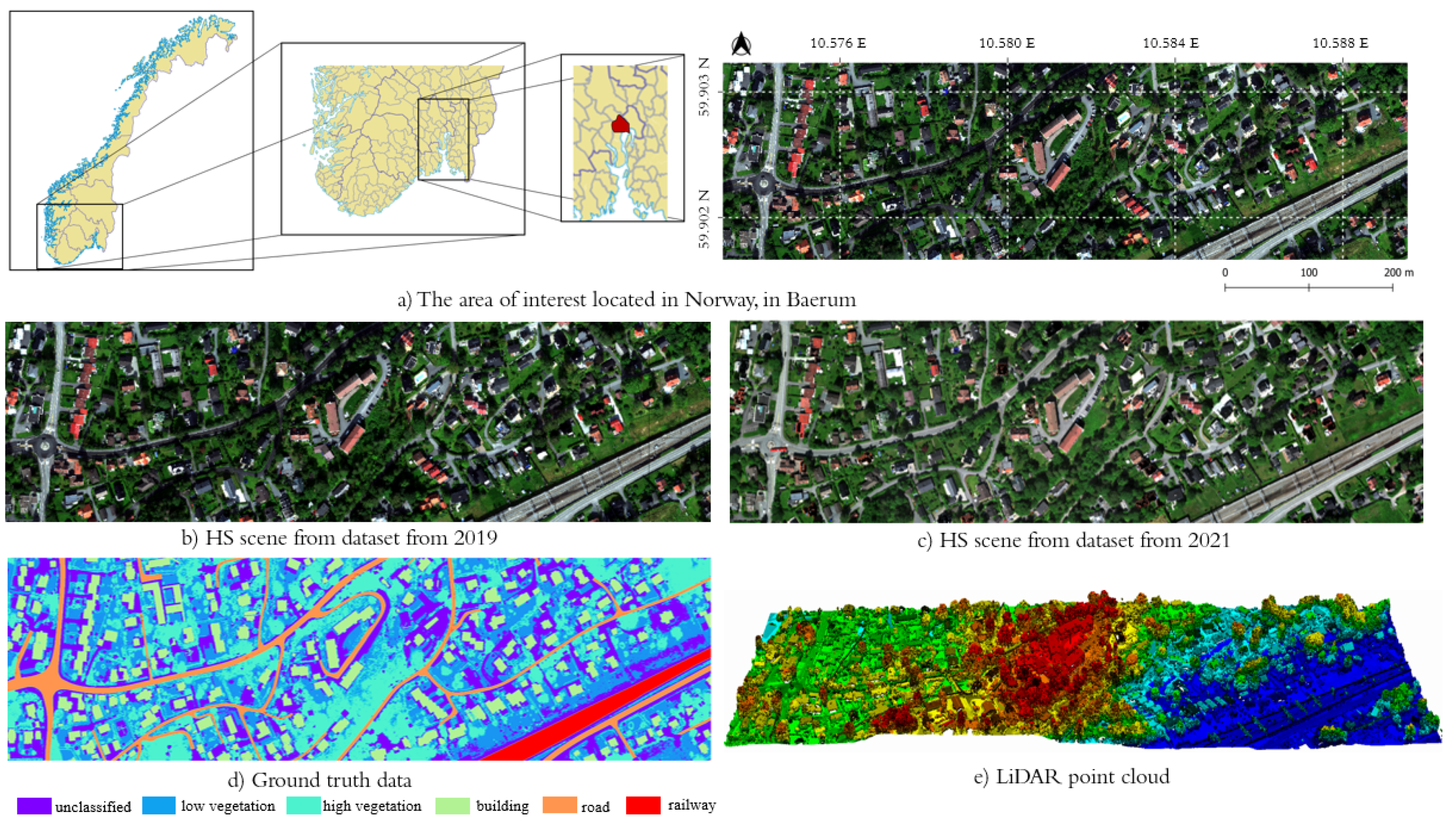
Figure 1. Our study area representing (a) the location of the area of interest, (b) the HS scene from 2019, (c) the HS scene from 2021, (d) the ground truth data, and (e) the LiDAR point cloud.
Remotesensing 15 00632 g001
Figure 2. Schematic workflow for multitemporal HL-Fusion at the feature level. According to flowchart guidelines, parallelograms represent data input/output, rectangles—process, and rhombi—decision.
Remotesensing 15 00632 g002
Figure 3. Schematic illustration of data augmentation created for training dataset for 64 × 64 pixel patches with 50% overlap. Image patches in the test dataset have an overlap of 0%.
Remotesensing 15 00632 g003
Figure 4. The clustering principle of intersections (green) and differences (blue) for two datasets, X1 and X2.
Remotesensing 15 00632 g004
Figure 5. Spectral unmixing example based on synthetic mixing result.
Remotesensing 15 00632 g005
Figure 6. (a) HS scene from a dataset from 2019, (b) corresponding ground truth data, (c) HS scene from a dataset from 2021, and (d) corresponding ground truth data.
Remotesensing 15 00632 g006
Figure 7. Segmentation results without data augmentation for the dataset from 2019 and 2021 for the ResU-Net showing (a) the first segmentation iteration for the dataset from 2019, (b) the first segmentation iteration for the dataset from 2021, (c) the second segmentation iteration for the dataset from 2019, and (d) the second segmentation iteration for the dataset from 2021.
Remotesensing 15 00632 g007
Figure 8. Segmentation results with data augmentation for the dataset from 2019 and 2021 for the ResU-Net showing (a) the first segmentation iteration for the dataset from 2019, (b) the first segmentation iteration for the dataset from 2021, (c) the second segmentation iteration for the dataset from 2019, and (d) the second segmentation iteration for the dataset from 2021.
Remotesensing 15 00632 g008
Figure 9. Spectral library of low and high vegetation, building (red, brown, and black roof tiles), road (yellow and white markings and asphalt), and railway generated after alignment after the II segmentation iteration. The bold black line in each plot represents the average image spectrum of each class.
Remotesensing 15 00632 g009aRemotesensing 15 00632 g009b
Figure 10. Change detection results for buildings and roads from FKB reference data to 2019 representing (a) buildings from the reference image (FKB), and (b) from 2019, (c) change detection for buildings, (d) roads from the FKB, and (e) from 2019, and (f) change detection for roads. Red color highlights changed pixels in the updated map.
Remotesensing 15 00632 g010
Figure 11. Change detection results for roads, low and high vegetation from 2019 to 2021 representing (a) buildings from 2019, and (b) from 2021, (c) change detection for buildings, (d) low vegetation from 2019, and (e) from 2021, (f) change detection for ow vegetation, (g) high vegetation from 2019, and (h) from 2021, and (i) change detection for high vegetation. Red color highlights changed pixels in the updated map. The green color represents pixels available only in the 2019 map (a map to be updated).
Remotesensing 15 00632 g011
Figure 12. Simulated change in the dataset from 2021. The red dashed rectangle represents an added building in place of low/high vegetation.
Remotesensing 15 00632 g012
Figure 13. An example of vegetation covering the road marked with a white dashed rectangle.
Remotesensing 15 00632 g013
Figure 14. Improvement of the shape of an object on example building detection marked with a dashed white rectangle.
Remotesensing 15 00632 g014
Table 1. Intersection endmember defined classes.
Defined ClassIntersection EM
roadEMi0-EMi9
buildingEMi10-EMi19
low vegetationEMi20-EMi29
high vegetationEMi30-EMi39
railwayEMi40-EMi49
Table 2. Segmentation results without data augmentation for the dataset from 2019 and 2021 for the ResU-Net model based on MCC calculated for each class (the range scales from −1 to 1) and overall F1 score (the range scales from 0 to 1).
ColorDataset20192021
Segmentation IIIIII
Low vegetation0.790.810.70.81
High vegetation0.920.920.760.91
Building0.880.940.920.98
Road0.780.890.820.91
Railway0.8510.990.98
F10.8180.8310.7520.776
Table 3. Segmentation results with data augmentation for the dataset from 2019 and 2021 for the ResU-Net model based on MCC calculated for each class (the range scales from −1 to 1) and overall F1 score (the range scales from 0 to 1).
ColorDataset20192021
SegmentationIIIIII
Low vegetation0.720.750.80.81
High vegetation0.940.970.950.97
Building0.970.990.990.99
Road0.920.950.990.99
Railway1111
F10.8140.8430.8860.892
Table 4. The segmentation results of a simulated dataset from 2021.
ColorDataset2021
Low vegetation0.79
High vegetation0.92
Building0.97
Road0.99
Railway1
F10.859
Disclaimer/Publisher’s Note: The statements, opinions and data contained in all publications are solely those of the individual author(s) and contributor(s) and not of MDPI and/or the editor(s). MDPI and/or the editor(s) disclaim responsibility for any injury to people or property resulting from any ideas, methods, instructions or products referred to in the content.