The Correlation between Ionospheric Electron Density Variations Derived from Swarm Satellite Observations and Seismic Activity at the Australian–Pacific Tectonic Plate Boundary

Abstract

Swarm electron density (Ne) observations from the Langmuir probe (LP) can detect ionospheric disturbances at the altitude of a satellite. Along-track satellite observations provide a large number of very short observations of different places in the ionosphere, where Ne is disturbed. Moreover, different perturbations occupy various Ne signal frequencies. Therefore, such short signals are more recognizable in two dimensions, where aside from their change in time, we can observe their diversity in the frequency domain. Spectral analysis is an essential tool applied here, as it enables signal decomposition and the recognition of composite patterns of Ne disturbances that occupy different frequencies. This study shows a high-resolution application of short-term Fourier transform (STFT) to Swarm Ne observations in the Papua New Guinea region in the vicinity of earthquakes, tsunamis, and related general seismic activity. The system of tectonic plate junctions, including the Pacific–Australian boundary, is located orthogonally to Swarm track footprints. The selected wavelengths of seismically induced ionospheric disturbances detected via Swarm are compared with the three sets of three-month records of seismic activity: in the winter solstice of 2016/2017, when seismic activity was highest, and in the summer solstice and vernal equinox of 2016, which were calmer. Moreover, more Swarm data records are analyzed at the same latitudes for validation purposes, in a place where there are no tectonic plate boundaries that are orthogonal to the Swarm orbital footprint. Additional validation is supplied through Swarm Ne observations from completely different latitudes, where the Swarm orbital footprint orthogonally crosses a different subducting plate boundary. Aside from the seismic energy, the solar radio flux (F10.7), equatorial plasma bubbles (EPBs), and geomagnetic ap and Dst indices are also reviewed here. Their influence on the ionospheric Ne is also found in Swarm observations. Finally, the Pearson correlation coefficient (PCC), applied to the pairs of 3-month time series created from Swarm Ne variations, seismic energy, ap, Dst, and F10.7, summarizes the graphical inspection of mutual correlations. It points to the predominant correlation of Swarm Ne disturbances with seismicity, especially during nighttime. We show that most of the Ne disturbances at a selected wavelength of 300 km correlate more with seismicity than with geomagnetic and solar indices. Therefore, Swarm LP can be assessed as being capable of observing the lithosphere–atmosphere–ionosphere coupling (LAIC) from the orbit.

1. Introduction

Studies of seismically induced ionospheric disturbances (SIIDs) are typically limited to selected large earthquakes or to the list of events that have a significant magnitude and directly trigger local SIIDs. However, tectonic processes are very complex and related to various types of motions of the Earth’s lithosphere, as well as to the generation of electric charge and chemical reactions [1,2,3]. The accumulated energy is released from the lithosphere and generates acoustic waves and atmospheric gravity waves that may travel to the atmosphere through weak zones in the Earth’s crust that are located at tectonic plate boundaries [4]. These waves cause disturbances in the temperature, pressure, and electromagnetic field [5,6]. The generated atmospheric gravity waves propagate right up to the ionosphere. When these waves reach the ionosphere, they cause detectable changes in the electron density (Ne) and total electron content (TEC). A strong electric field can also be induced prior to an earthquake, and this is characterized by radioactive particle emanation (mainly radon) and increased conductivity, causing electric field anomalies [2,7]. There is also an electrostatic channel of seismo-ionospheric coupling described by Freund [8] and Hayakawa et al. [7], in which positive ionization holes are generated from the stressed ground. According to their origin, the ionospheric disturbances can be divided into two categories. The first one refers to the Sun’s activity, e.g., the solar flare eruption or coronal mass ejection, while the second one includes anthropogenic and natural events on the Earth. Both categories have different scales and duration times. The disturbances from Earth-based sources last for several hours or days, and their scale is about hundreds or thousands of kilometers [9,10]. Importantly, the ionospheric anomalies caused by earthquakes or volcano eruptions arise from a process called lithosphere–atmosphere–ionosphere coupling (LAIC) [11,12,13,14,15].

Due to several tens of satellites and thousands of stations, ground-based Global Navigation Satellite System (GNSS) data are the most promising for research on SIIDs. This fact comes from one main reason: ground-based GNSS observations provide the only reliable spatial view of SIIDs and enable recognition of their spatial shapes and movement velocity. A vast majority of undertaken research related to SIID analyses based on ground-based GNSS data was focused on the identification of different kinds of ionospheric waves and their propagation after large earthquake events [9,13,16,17,18,19,20,21]. Some of the authors apply statistical analyses of TEC responses to the earthquakes over a longer time span, which are typically a basis for studies on earthquake precursors and preseismic disturbances [22,23]. The application of ground-based GNSS data is focused on the locations where the stations provide spatially dense observations. There is, however, a limited number of dense GNSS networks. The ground GNSS stations have a heterogeneous distribution worldwide. Moreover, there are also many places along the subducting plate boundaries where GNSS stations are very sparse or unavailable.

A low density of GNSS stations significantly impedes the identification of SIIDs in many interesting places and limits the study of them on a global scale. However, the observed increasing number of explorer satellite missions dedicated to global ionosphere observation can significantly extend the global approach. Low Earth orbiting (LEO) satellites can visit all the regions of the Earth, which is interesting for the global investigation of LAIC. An example of a completed satellite mission that was designed to monitor the variations in the atmosphere related to earthquakes is the French DEMETER (Detection of Electromagnetic Emissions Transmitted from Earthquake Regions) mission, active from 2004 to 2010. The DEMETER satellite had been orbiting at a Sun-synchronous circular orbit, having an approximate altitude of 710 km and inclination of 98.2°. The scientific payload on the DEMETER satellite included a Langmuir probe (LP) measuring Ne and electron temperature. DEMETER provided observations of electromagnetic fluctuations related to earthquakes [24,25]. DEMETER data have also been examined in various ways to define the perturbations of the ionosphere caused by acoustic gravity waves from earthquakes [24,25,26,27]. The ionospheric disturbances associated with preseismic activity were also investigated in a study based on DEMETER data, conducted by Zhang et al. [28], and studies combining GNSS and DEMETER data conducted by Akhoondzadeh et al. [29] and Ibanga et al. [30].

The existing satellite missions that include LPs amongst the scientific payloads are the first European Space Agency (ESA) constellation mission for Earth observation called Swarm [31,32] and the Chinese–Italian space mission named the China Seismo-Electromagnetic Satellite (CSES) [33]. The Swarm constellation comprises three satellites, which compose the fifth Earth Explorer mission that was approved in ESA’s Living Planet Program, and they were successfully launched on 22 November 2013. The orbits of Swarm Alpha (Swarm A) and Charlie (Swarm C) have an initial altitude of 460 km and inclination of 87.4°, whereas Swarm Bravo (Swarm B) runs at an altitude of 530 km and at a 88° inclination angle. The research objective of the Swarm mission is to provide the best-ever survey of the geomagnetic field and electric field in the atmosphere using precise magnetometers and electric field instruments. Very frequently, Swarm data studies related to earthquakes incorporate magnetic data from all three satellites. There is published evidence of precursory signals in the magnetic data [34,35], as well as works referring to co-seismic signals in the magnetic field [36,37,38]. Zhu et al. [35] referred to the extended number of earthquakes, including ones of smaller magnitudes, and showed one example of spectral recognition of disturbed signals, which is also an objective of our current study. Ghamry et al. [39] analyzed the seismic precursory magnetic anomalies measured onboard Swarm together with different additional data, like thermal anomalies from other explorer satellites, like Terra and Aqua. Aside from the magnetic sensors, the Swarm payload also includes LPs and GNSS receivers for precise orbit determination, which can be used to observe in situ ionospheric Ne and topside TEC, respectively. Stanica et al. [40] jointly studied the variations in magnetic and electric field parameters as precursory to some moderate-magnitude earthquakes in Romania. A stronger event in Mexico was investigated by Marchetti and Akhoondzadeh [41] with the application of magnetic and Ne data, whereas Marchetti et al. [42] have studied seismic sequences in Italy using a variety of Swarm observations. In terms of earthquake number, an extended study was conducted by De Santis et al. [43], who prepared a statistical assessment of magnetic and Ne disturbances related to 12 earthquakes of various magnitudes. The satellite of the CSES mission that is dedicated to monitoring electromagnetic fields was launched on 2 February 2018. It is equipped with instruments that are similar to Swarm’s, capable of observing electric and magnetic fields from a Sun-synchronous orbit at an altitude of around 500 km, with an inclination of around 97.3°. There are already works based on CSES data related to selected earthquakes by Huang et al. [44] and groups of similar large earthquakes by Yan et al. [45]. Xiong et al. [46], as well as Yan et al. [45], analyzed CSES data focusing on precursory signals with respect to earthquakes. Marchetti et al. [42] have also investigated possible LAIC effects prior to the M = 7.5 earthquake using, among the others, Swarm and CSES datasets. De Santis et al. [47] have prepared a statistical spatiotemporal analysis of CSES-observed disturbed ionospheric signals due to an earthquake occurrence, which is quite analogous to the analyses made with Swarm data in [48].

He et al. [49] significantly extended the analyses of Swarm Ne disturbances in relation to seismic activity. They analyzed the global distribution of Swarm Ne disturbances and compared them to areas of higher and lower seismic activity rather than to specific earthquakes. Their analysis has a commonality with our current study, as we also try to focus on the continuous global seismic activity of various magnitudes. They analyzed global Ne disturbances statistically, with no spectral tools. In contrast, we try to analyze one important place locally and decompose disturbances in their frequency domain. The advantage of LEO satellites is that they provide data in places that cannot be reached by ground GNSS observations. The orbital tracks of LEO can reach all seismically active zones of the world. A drawback of LEO is that the satellite data are dense only along the orbital tracks. The one-dimensional nature of LEO along-track Ne observations and sometimes the limited chance for spatiotemporal correlation due to the nonrepeating orbits leads to a strong requirement for spectral analysis for better recognition of the signals. The spectral analysis of residual signals can be found several times in the studies on seismically induced ionospheric disturbances in ground GNSS data [17,18,50]. It is possible that the processing of LEO data requires a spectral approach more than time series from a ground station do, as the disturbed signal is less pronounced in transient LEO observations. Fortunately, the frequency domain has been analyzed more frequently in LEO data in recent years [35,51,52,53,54]. These studies are encouraging us to take a further step and try a spectral classification of specific patterns that refer to different Ne and TEC signal disturbances. The proposed research aims at the investigation of LAIC via short-term Fourier transform (STFT) analysis of disturbed Ne, measured by Swarm over tectonic plate boundaries. This facilitates the analysis of seismically induced ionospheric disturbances with respect to larger earthquakes and their groups within the earthquake catalogue. The validation of disturbances detected by Swarm satellites in times of strong earthquake activity is based on the analysis of analogous data from the periods and places of lower seismic activity. The spectral decomposition of the disturbed signal can significantly help in the inspection of spectral behavior of ionosphere anomalies and the identification of the most frequent wavelengths of their occurrence. These determined spectral patterns, after more extended research in the future, can be classified as different types of disturbed signals, which was previously suggested in [17,18,51,52]. The extended spectral analyses of LEO electric field data can, in the future, help in the recognition of satellite data disturbances related to different seismic activities like mainshocks, aftershocks, preseismic activity, and also to moderate seismic activity in the vicinity of tectonic boundaries.

The tectonic plate boundaries are weak places of the Earth’s lithosphere and can trigger preseismic, co-seismic, and post-seismic ionospheric disturbances. Swarm satellites visit these boundaries at different longitudes on the subsequent days and, due to their high speed, collect short samples of observations along their orbits. Therefore, the current study investigates two issues: firstly, a comparison of three-month-long records of Ne disturbances to the continuous seismic activity and not only to the largest earthquakes; secondly, a preliminary STFT recognition of Swarm Ne disturbances. In both cases, Swarm-derived Ne are compared with continuous seismic records acquired from the United States Geological Survey (USGS) in the regions of interest. This study investigates nine three-month datasets, but primarily one example of a nearly latitudinally located boundary of the Australian and Pacific Plate that is rich in nearby minor plates and is very active. Swarm A/C and B tracks over this boundary are analyzed within a longitude range of around 30°. The dependence of the seismicity level on the season is very often discussed among researchers. Moreover, seasonal periodicities were already estimated in some works [55,56]. Therefore, at the beginning, we apply three-month-long series of nighttime Swarm data in Papua New Guinea from three different seasons of the year and compare them with the corresponding lists of earthquakes with a M ≥ 5.0. The fourth and fifth data series are from the Aleutian Islands at alternative latitudes and Africa at alternative longitudes. These series are analyzed to better validate Swarm’s sensitivity to different seismic activity levels and solar conditions. The remaining four datasets are derived from daytime Swarm passes in Papua New Guinea and analyzed with respect to daytime signal sensitivity. To observe the influence of various factors, Swarm Ne disturbances are analyzed in the time domain together with seismicity, solar radio flux (F10.7), geomagnetic ap and Dst indices, and the ionospheric bubble index (IBI), indicating equatorial plasma bubbles (EPBs) along the satellite tracks [57,58,59]. The primary graphical inspection of the correlation of Swarm Ne disturbances with seismicity or with ap, Dst, and F10.7 is summarized by the Pearson correlation coefficients (PCC), calculated between all pairs of parameters and also between their 5, 7, and 10-day averages. PCC validated mutual correlations over time between Swarm Ne variations, seismicity, and solar and geomagnetic parameters. The most pronounced correlation is observed between Swarm Ne irregularities and the cumulative seismic energy at nighttime. This is promising for the future tracking of seismic activity over tectonic plate boundaries using spectrally analyzed LEO data but is at the same time challenging and needs more research employing global data.

2. Methodology

This work is based on the calculation of time-variable power spectral density (PSD) of the high frequencies (short periods) of Swarm Ne 2 Hz data from LPs, starting from around 65 s. We use wavelengths as frequency domain units, mainly for a better geometrical understanding of the disturbance size found at specific frequency. This unit is derived from the recalculation of Swarm data time units to distances along the orbit, using Swarm speed. It is therefore possible that two frequency domain units are applied alternately, i.e., period and wavelength. However, the term “period” is used also in reference to selected time epochs, which can be recognized from the context. The high-pass filtering of selected track parts of Swarm LP data is based on discrete Fourier transform (DFT), which is more universal than wavelets in the band-filtering processes, as it can decompose discrete signals in terms of sinusoids or complex exponentials. The signal of time function x(t) can be decomposed into frequency responses X(ω), sampled for the entire ω spectrum. These responses can also be transformed back exactly to x(t) via the inverse Fourier transform. The selected signal band can be subtracted from the data, which, contrary to simple methods of detrending, e.g., moving average or polynomial, removes exactly the part of the signal that we want to remove in terms of a frequency band. The nonspectral methods can remove arbitrary frequencies/wavelengths if the signal variances and spectral content differ in different places.

The amplitude of signal responses in the frequency domain provides the PSD at individual wavelengths. The amplitude of spectral peaks usually varies with time, and this is the case with Swarm signals recorded along its orbital track. We have to carefully and accurately analyze the time-evolution of ionosphere disturbances measured by Swarm, because the speed of the satellite is fast with respect to sensed disturbances, and therefore, signal samples are composite but short. Time-variable PSDs plotted over time have the ability to map such changes in the frequency domain. The windowed STFT is a modification of the DFT method, which computes the spectrum of overlapping segments of the time series. The output of STFT is the short-term, time-localized evolutionary PSD. The data sequence to be transformed is multiplied using a window function, which is nonzero for only a short period of time [60,61]. The STFT of the signal is computed as the window is sliding along the time axis, resulting in a two-dimensional representation of the signal. Mathematically, this is written as

$$\begin{array}{ccc}{STFT}_{x,f,t}={\sum }_{n=0}^{N-1}{x}_n{w}_{n-t}{W}_N^{-fn}& & f=\mathrm{1,2},\dots ,N-1\end{array}$$

(1)

where

$$W_N=e^{\frac{i2\pi }{N}}$$

(2)

and $w_n$ is a discretized window function, and t is its time index. The window applied in this study is the Tukey window. This window, also known as the cosine-tapered window, can be regarded as a cosine lobe of width $\frac{r}{2}\left(N-1\right)$ that is convolved with a rectangular window of width $\left(1-\frac{r}{2}\right)\left(N-1\right)$. The equations defining Tukey window are

$$w_{TU}\left(n\right)=\left\{\begin{array}{ccc}\frac{1}{2}\left[1+cos\left(\frac{2\pi }{r}\frac{n-1}{N-1}-\pi \right)\right]& ,& n<\frac{r}{2}\left(N-1\right)+1\\ 1& ,& \frac{r}{2}\left(N-1\right)+1\le n\le N-\frac{r}{2}\left(N-1\right)\\ \frac{1}{2}\left[1+cos\left(\frac{2\pi }{r}-\frac{2\pi }{r}\frac{n-1}{N-1}-\pi \right)\right]& ,& N-\frac{r}{2}\left(N-1\right)<n\end{array}\right\}$$

(3)

where r is a value between 0 and 1. STFT of a data sequence $x_n$ describes its local spectral content near the moment t as a function of $f$. Moving the center of the window $w_{n-t}$ along the real line (of real units) allows for obtaining snapshots of the time-frequency behavior of $x_n$. STFT is used in the calculation of the amplitude of frequency spectrum for each sample. These spectra then form a 2-D shape that depends on the window size and overlay size. This corresponds to the computation of the STFT squared magnitude of the signal sequence $x_n$—that is, for a window width n:

$${SP}_{xx,f,t}={\left|{STFT}_{x,f,t}\right|}^2$$

(4)

The size and shape of the analysis window can be modified depending on the purpose. A shorter window will produce more accurate results in terms of timing at the expense of the precision of frequency representation. A longer window will provide a more precise frequency representation at the expense of precision in time location.

3. Swarm and Ancillary Data

The region of Papua New Guinea is located at the junction of four main tectonic plates: the Australian, Pacific, Eurasian, and Philippine Sea Plate. There are also several smaller plates, which makes this region especially seismically active. The main time period selected for the analysis due to the strong seismic activity is the winter period covering November and December of 2016 and January of 2017. The two additional three-month periods for the validation are the spring period from February to April of 2016 and the summer period extending from May to July of 2016. The general M = 5.0 threshold for the selection of earthquakes in this work is assumed approximately on the basis of existing works on the sensitivity of ground GNSS data to seismic activity (see: [14,62]), as well as from the recent works on the sensitivity of Swarm magnetic data to earthquakes [37,42]. November of 2016 is relatively seismologically quiet and includes a week during which no earthquake of M ≥ 5.0 was recorded in the investigated region. December 2016 in Papua is very active seismologically, with two earthquake events having magnitudes of 7.8 and 7.9, both triggering tsunamis. January is not as quiet as November, including more earthquakes with M ≥ 5.0. It includes also one having a M = 7.9; however, this was deep, with no following aftershocks. It should be pointed out that based on the earthquake number, the tectonic plate junction seems to have been more relaxed in January 2017 than before December 2016. February–April of 2016 and May–July of 2016 are seismically lower active periods compared with to winter. However, in this especially active region, these periods also include a significant number of earthquakes exceeding 5.0 and 6.0 magnitudes. The earthquake records for all three seasons in the Papua New Guinea region are selected using the geographical window of 10°N–30°S and 130°E–170°E. Additionally, two other regions of Swarm data analysis are selected for validation and confutation purposes. These regions use geographical windows selecting Swarm Ne data at the equatorial latitudes first, but at a significantly different longitude, and second, at an absolutely different latitude, far from the equator. For the African region, we applied the window of 10°N–30°S and 0°E–40°E. The region of Aleutian Islands was selected using the window of 30°N–70°N and 160°E–130°W. We used geodetic latitudes, as the difference with respect to geomagnetic ones is less significant here than the selection of the place that is free from a latitudinally aligned tectonic plate boundary, which is Africa. The data in both ancillary regions cover the primary period of Papua New Guinea data from November 2016 to January 2017.

The list of earthquakes is extracted from the Search Earthquake Catalog, which is available from the USGS website. There were almost 200 earthquakes in the Papua New Guinea region with a magnitude equal to or above M = 5.0 from the beginning of November 2016 to the end of January 2017 (Figure 1). A significant part of these earthquakes included aftershocks and occurred just after 8 and 17 December 2016. The orbits of Swarm satellites, which have an inclination between 87° and 88°, pass the boundary of two major subducting tectonic plates (Australian and Pacific) at an angle that is close to 80°.

The analysis of the Swarm data in the Papua New Guinea region is based on the LP data from Swarm Level 1b Electric Field Instrument (EFIxLP). The longitude (λ) of the Swarm satellite pass does not repeat the next day at the same time, and moreover, it is not exactly the same. Therefore, we selected Swarm passes from consecutive days of the three-month periods, having close longitudes and being recorded at a similar time of the day. The selection of Swarm A and C orbital tracks for the analysis of winter solstice starts from Swarm A and C trajectories recorded on 17 December 2016, which both took place 40 min. after the largest M = 7.9 earthquake occurred close to the eastern coast of New Ireland island in Papua New Guinea (10:51 UTC, which is 20:51 local time (LOC)). Then, for each satellite (A/C), an additional 90 Swarm tracks from the preceding and subsequent days are selected (1 November 2016–30 January 2017). The threshold difference in the 90 adjoined tracks in the time unit, in relation to that on 17.12, is set to a maximum of 4.4 h, whereas the allowed difference in longitude is a maximum of 20°. The range of latitudes of the 91 selected tracks is approximately between 25°N and 45°S (Figure 2a). This selection produced 91 track sections, shown in Figure 2a, and the same rule with reference Swarm A/C tracks is applied in a more quiet region of the African Plate to select a similar number of tracks at very similar latitudes (Figure 2b). In order to keep Figure 2a transparent, the date labels are only shown for the eight selected days and are also presented in Figure 4, Figure 5 and Figure 6 including the most significant disturbances within the selected period. In the third selected region, which is the junction of the Pacific Plate and the North American Plate located at completely different latitudes, the reference Swarm track is selected from the 17th day of the middle month (Figure 2c). The longitude differences and time differences of the adjoined tracks in relation to the reference track are the same as for the primary region. The Swarm orbital track selections in the Papua New Guinea region for the other seasons of 2016 are prepared in exactly the same way, starting with the track within very similar latitudes on the 17th day of the middle month, and adjoining remaining Swarm passes at close longitudes using the same longitude and time separation maxima. Additionally, the same rule is applied for the selection of the opposite daytime tracks that were investigated, aside from the above-mentioned nighttime or nearly nighttime passes. Neither the track selection in the summer solstice and vernal equinox nor the daytime tracks need to be plotted in the figures, as these tracks follow the same rule that can be seen in Figure 2a and Figure 3a. They pass tectonic plate boundaries within very similar latitudes, similar longitudes, and similar times, dependent on the actual Swarm trajectory, but always refer to the selected half of the day.

The selection of Swarm B tracks starts from the Swarm B trajectory recorded on 8 December 2016, approximately 30 min. before the largest M = 7.8 earthquake in the Solomon Islands region near Papua New Guinea, which occurred close to the western coast of San Cristobal Island (17:38 UTC—3:38 LOC). Then, an additional 90 Swarm tracks from the preceding and subsequent days (1 November 2016–30 January 2017) are selected. The range of latitudes of the 91 selected tracks is approximately the same as for the Swarm A/C pair. The allowed between-track differences in time and longitude with respect to a trajectory of 8.12 are also the same. The tracks of Swarm B are grouped in a slightly different way than Swarm A/C, as the orbit repetition cycles of Swarm B (Figure 3a) differ in comparison to those for Swarm A/C. The selection of Swarm B passes in a more seismically quiet area is shown in Figure 3b. The selection of Swarm B passes at different latitudes is shown in Figure 3c. It should be pointed out that the reference track selection is unified with the rules of the Swarm A/C reference track selection, which is always selected on the 17th of the middle month. The selection of Swarm B tracks in the summer of 2016, spring of 2016, and during the daytime has followed the same rule of very similar latitudes, similar longitudes (±20°), and similar times, separated by 4.4 h from the reference track. Such an apparently long separation in time is necessary to find Swarm tracks with success on every day and to have the smallest number of gaps.

Figure 3. (a) Selection of descending (nighttime) Swarm B tracks over Papua New Guinea between 1 November 2016 and 30 January 2017. The tracks are selected to have the closest possible time of the day and longitude to the first selected track just before M = 7.8 mainshock. The red triangles denote earthquakes above magnitude 6.5. (b) Selection of Swarm B tracks at the same latitudes and local time in a more seismically quiet region. The red triangles denote earthquakes above magnitude 4.0. (c) Selection of Swarm B tracks at the high and middle latitudes. The red triangles denote earthquakes above M = 4.5.

Figure 3. (a) Selection of descending (nighttime) Swarm B tracks over Papua New Guinea between 1 November 2016 and 30 January 2017. The tracks are selected to have the closest possible time of the day and longitude to the first selected track just before M = 7.8 mainshock. The red triangles denote earthquakes above magnitude 6.5. (b) Selection of Swarm B tracks at the same latitudes and local time in a more seismically quiet region. The red triangles denote earthquakes above magnitude 4.0. (c) Selection of Swarm B tracks at the high and middle latitudes. The red triangles denote earthquakes above M = 4.5.

Figure 2 and Figure 3 present the rule of selection of Swarm A/C and B trajectories—one each day at a similar time of the day. The three-month sets of around 91 trajectories for different satellites, regions, and times of the day are then prepared for the comparison of ionospheric Ne perturbations to seismicity, solar activity, EPBs, and geomagnetic activity. Three seasons are analyzed in Papua New Guinea in the nighttime and daytime, which provides six three-month series. Two other series come from the winter solstice in Africa and Aleutian Islands. The other dataset includes daytime data in Papua New Guinea, with Ne irregularities analyzed at the same frequency as the nighttime data. Three other daytime analyses apply sampling at the higher frequency.

4. Spectral Patterns of Swarm Ne Disturbances during Nighttime of the 2016–1017 Winter

From the winter set of the 91 trajectories within the three-month period, eight are selected for each Swarm spacecraft to illustrate the spectral characteristics of the most important moments in the spectrograms (see labels on Swarm passes in Figure 2 and Figure 3). Besides that, the measures of the disturbance scale for the entire three-month comparisons with seismicity are also determined from the spectrograms as the maximum PSD of Ne disturbances at the selected wavelength (from here, simply called Swarm Ne PSD). The orbital tracks from the three Swarm satellites are selected for consecutive days at a similar time of the day (±4.4 h), e.g., one for each of the 91 days from 1 November 2016 to 30 January 2017. The Ne data collected along these orbital arcs are high-pass filtered and then spectrally analyzed via STFT. All spectrograms describing a varying PSD of ionospheric Ne are sampled for further joint processing with seismicity, solar conditions, and the geomagnetic index. However, as three months produce 273 trajectories, this section shows the spectrograms from three Swarm satellites only for the selected eight most important days from the winter solstice in the region of Papua New Guinea (Figure 2a, Figure 3a, Figure 4, Figure 5 and Figure 6). In order to avoid a dominating PSD at long wavelengths, which often disturb viewing shorter wavelengths in spectrograms or scalograms, the data are high-pass filtered, which removes the signals with wavelengths that are longer than 500 km. The approximate recalculation from the period of 65 s. to wavelength is based on the speed of the Swarm at its flight altitude, which is around 7.6 km/s. This 500 km wavelength threshold is fixed approximately, but its choice is based on the most frequent width of seismic gravity waves located in the ionosphere close over their lithospheric source. This width usually does not exceed 500 km [9,20,63]. On the other hand, the wavelengths of similar widths are detectable in TEC series before the earthquakes as well [64,65]. The latter fact provides information about the usefulness of such selected thresholds in the detection of preseismic, co-seismic, and post-seismic irregularities. Moreover, the use of a reasonably short lower bound of the filter must be selected to exclude natural low-frequency Ne signals, which are dependent on the Sun and geomagnetic activity. This is important, especially at equatorial latitudes in the region of equatorial ionization anomaly (EIA). The high-pass filter is based on the decomposition of the signals via DFT.

Figure 4, Figure 5 and Figure 6 present the spectrograms calculated with the use of STFT and the Tukey window with its main parameter r = 0.4 (Equation (3)). The width of the Tukey window is set to 180 s (~1400 km), and the period/wavelength range is set from 10 s (~80 km) to 120 s (~920 km). This relatively long window size slightly blurs the moment of the occurred disturbance but enables a significantly better spectral resolution of the residual Ne spectrogram at longer wavelengths. It should be pointed out here that scales of the spectrograms, as relative quantities, are omitted to avoid redundant information, but are exactly the same. The time in Figure 4, Figure 5 and Figure 6 is given in UTC along the horizontal axis, but easy recalculation can be performed to the local time (LOC) by adding +10 h. Figure 4, Figure 5 and Figure 6 show the spectrograms of the selected, most significant passes over the region, in the sense that these Swarm tracks observed the most evident disturbances that were co-located with seismic activity in the region of Papua New Guinea between November 2016 and January 2017. The maxima of the PSDs of these disturbances detected by Swarm at a 300 km wavelength (Swarm Ne PSD) are summarized further in Figure 7 in Section 5. The days of 19 and 20 November 2016 are days of low ap and Dst indices and moderate seismic activity. A single week of relaxation from earthquakes equal to or stronger than M = 5.0 starts here, and the last earthquake with an M = 5.5 happened in the region on November 17, just before this quiet week. Swarm A finds a moderate disturbance on November 19 (Figure 4a) and a quite large, disturbed signal on November 20 (Figure 4b). Swarm C, flying close to Swarm A, also sees these signals (Figure 6a,b). In general, Swarm C signals are similar, but the one on November 20 is weaker, which may suggest a quite fast change in the signal in time (Figure 6b). Swarm B, which was visiting the region around four hours later on these days, observed a weaker disturbed signal on November 19 (Figure 5a), but one that was spectrally similar to that seen by Swarm A on November 20 in Figure 4b. These similarities can suggest to some degree that we see the same changing disturbance in Figure 4b, Figure 5a and Figure 6b. The relative longitudes of the Swarm A/C pair and Swarm B in the above case do not differ much (Figure 2a and Figure 3a). The longitude of Swarm A on November 20 was around 150°, whereas the longitude of Swarm B on 19 November was around 160°. This is not significant, and it is theoretically possible that Figure 5a presents the spatiotemporal evolution of the signal shown in Figure 4b.

The first earthquake with M = 5.0 occurred after a one-week period that was free from 5.0+ earthquakes and happened in the Papua New Guinea region on November 27, after a maximum ap increase to 5+ on November 25 and respective Dst variation. Figure 4c shows the quasi-trapezoidal shape of the PSD of a large Ne disturbance detected by Swarm A at an around 400 km wavelength, with a weaker disturbance at a wavelength that was shorter than 300 km. Figure 6c presents a weaker and moderately similar perturbation for Swarm C, which, however, occupies the same two wavelengths. Figure 5c shows an ionosphere disturbance sensed by Swarm B around 4 h later than Swarm A/C. This perturbation is latitude-shifted and weaker but also quite similar in its PSD shape and wavelengths to those in Figure 4c and Figure 6c. One should take into account the different altitudes of the Swarm A/C pair and Swarm B, which can obviously contribute to differences in the disturbance shape between A/C and B. Although different altitudes of the satellites result in the observations of different parts of the Ne vertical profile, a probable consistency can be found between Figure 4c, Figure 5c, and Figure 6c, suggesting the same origin of the signals.

Further large PSD values in Swarm A observations are found on 8 December 2016 (Figure 4d) when the seismic activity increased; this was five hours before one of the two largest earthquakes over the analyzed period. This earthquake induced a tsunami that was recorded by the National Oceanic and Atmospheric Administration (NOAA) tide gauges. The earthquake happened in Kira Kira, Solomon Islands, at 17:38 UTC (3:38 LOC) and had M = 7.8 and depth = 41 km. The passes of Swarm A and C were there around five hours before the mainshock (Figure 4d and Figure 6d). The disturbance at that time was strong, very similar for A and C, and occupying longer wavelengths in the filtered frequency domain (300–400 km) for a significant time of the pass, but also some that were shorter than 300 km (Figure 4d and Figure 6d). Additionally, the PSD of the large Ne peak in Figure 4d appears like a mirror reflection of the PSD in Figure 4c, which suggests the observation of a very similar perturbation of the ionosphere crossed by Swarm A from two opposite directions. The signal observed by Swarm C (Figure 6d) is very similar to that observed by Swarm A (Figure 4d), and we can be sure that it refers to the same disturbance. The Ne signals were different 4.5 h later, which was half an hour before the earthquake and before Swarm B visited the region (Figure 5d). Figure 5d shows the more disturbed Ne signal of Swarm B, which has clearly separated short wavelengths around 150 and 180 km. This fact strongly suggests new perturbations aside from those found 4.5 h before by Swarm A/C. These perturbations can originate from different physical phenomena, and their presence can be confirmed with other observations of physical and chemical parameters, including the local ones. At least, the possibility of a higher emission of radon can be taken into account, as it is generated continuously in any geological structure, and its highest emission can also be found just before the strong earthquakes [2]. Figure 4e and Figure 6e still show quite large disturbances on the next day (December 9) for Swarm A and C, which occupy the wavelengths around 300–400 km. Figure 5e presents a much more dispersed and weaker residual signal of Swarm B on December 9. We should, however, remember the longitudes, which differ more in the case of Swarm A/C than in the case of Swarm B (Figure 2a and Figure 3a). The footprint of the Swarm A/C pair on December 9 is quite far from the corresponding one on the previous day.

Figure 4f and Figure 6f present an increased PSD at various frequencies of residual Ne on 17 December 2016, which was 40 min. after the major earthquake occurred at 10:51 UTC (20:51 LOC) close to the island New Britain in Papua New Guinea, having M = 7.9 and a depth of 103 km. The PSD pattern in Figure 4f has a similar dispersion in frequency to that in Figure 5d for Swarm B, because it occupies at least three separated spectral bands. The common point of Figure 4f, Figure 5d, and Figure 6f is that all of these figures describe Swarm passes in the temporal proximity of major earthquakes. A characteristic feature of these disturbances is a high PSD magnitude at various wavelengths, including higher wavelengths somewhere between 100 and 300 km, which are probably wavelengths for gravity waves propagating to the ionosphere [20,63]. It should be pointed out that due to the complicated geometric relations and high Swarm speed, with respect to most seismic waves [13], we can interpret that Swarm measures a snapshot of the existing waves at each given moment. The selection of the wavelengths that are sensitive and corresponding to ionospheric disturbances in the Swarm signal has a preliminary character here. Thus, consideration of relative speeds of Swarm and gravity waves would be time-consuming and not necessarily effective, with no detailed knowledge of the expected disturbing wave width at Swarm altitudes. Summarizing the day of December 17, we can assess that the PSD of the disturbed signal from Swarm C in Figure 6f follows the same rule as Swarm A in Figure 4f and the one from Swarm B in Figure 5d, i.e., the signal is composed of many wavelengths. A very similar complex spectrum can also be observed for Swarm B in Figure 5f, but the PSD is much weaker there. However, a suspicion of a similar origin of the disturbances in Figure 5f must be verified through additional data investigation. On 18 December 2016, the signals seemed to occupy many frequency bands, but at the same time, they are dispersed over a larger area, which is noticeable in Figure 4g (Swarm A) and Figure 5g (Swarm B) but is less pronounced in Figure 6g for Swarm C. The spectra of the most noticeably dispersed disturbances in Figure 4g and Figure 5g are very similar, but different from that in Figure 6g. The reason for the moderate differences between Swarm A and Swarm C is not known at all, but there are some suspected origins, like instrumental problems or other disturbing factors.

Further proof that we can certainly expect a similar PSD of residual Ne from Swarm A and Swarm C can be observed on 8 January 2017. On that day, an earthquake with M = 5.9 occurred, and there was also geomagnetic disturbance, with the ap ranging up to 4.5. This stronger geomagnetic activity apparently does not affect Swarm A/C signals (Figure 4h and Figure 6h), or it affects them at longer already filtered wavelengths. Figure 4h and Figure 6h present almost the same PSD shape for Swarm A/C satellites, which confirms that STFT works well, and we can observe the same disturbance in the same place. There are also some unconfirmed EPBs indicated in the L2 IBI product (Figure 4h and Figure 6h), but they seem to not disturb the signal much at the time of their occurrence. Figure 5h for Swarm B shows no EPBs from the IBI product but a different, very high PSD of Ne, extended over around 30° along the satellite way. On the one hand, this disturbance reaches the tectonic plate boundary in the middle part of the spectrogram, but on the other hand, it starts over the Pacific, some hundreds of kilometers north of the tectonic plate boundary (Figure 3a). Therefore, it is suspected that a stronger geomagnetic activity has affected the Ne signal at the frequencies where we can detect seismic disturbances, thus resulting in mixed signals.

The most composite ionospheric disturbances in terms of a variety of disturbed wavelengths occur in the proximity of the two largest December earthquakes investigated in this work. Figure 4f and Figure 6f present the composite Ne disturbance detected via LPs onboard Swarm A and C around 40 min. after a M = 7.9 earthquake in Papua New Guinea, whereas Figure 5d shows the composite Ne disturbance in observations of Swarm B around 30 min. before the M = 7.8 earthquake in the Solomon Islands. In such cases, the signal is strongly modified and has large PSD of residual Ne at various wavelengths around 150, 200, 300, and 400 km. Figure 4, Figure 5 and Figure 6 include the original Ne signal from LPs to indicate the position of the disturbances with respect to EIA crests. It can be noticed that the positions of the perturbations are varied. The anomaly in Figure 4h occurs at the crest of the Ne plot, whereas the one just before the major earthquake in Figure 4f is located at the end of the crest. The strongest disturbance at an around 400 km wavelength in Figure 4d appears to be between the crests, whilst the strongest disturbances in Figure 4g are located along the slope of the EIA crest. The crests of the Ne profile along the Swarm track can also be relatively smooth, with no stronger disturbances, as is seen in Figure 4a, Figure 5b or Figure 5e. On the other hand, such signals, like that in Figure 4h, which are located at the Ne crest, are high-frequency signals. Therefore, we cannot exclude their common seismic origin with the signals of the same frequency located in other places, e.g., at the crest slope.

Figure 4. Spectrograms of LP Ne from selected Swarm A passes over Papua New Guinea. Frequencies are recalculated to km at the altitude of the spacecraft. The horizontal line is a wavelength of 300 km, selected for PSD sampling used in comparison to seismic record. Measured Ne values are shown in blue, and unconfirmed EPBs are shown as blue circles, which are drawn at 200 km wavelength to be well readable. The top axis represents UTC time, and the bottom axis represents latitude. Left axis labels refer to wavelength, whereas right axis labels refer to Ne.

Figure 4. Spectrograms of LP Ne from selected Swarm A passes over Papua New Guinea. Frequencies are recalculated to km at the altitude of the spacecraft. The horizontal line is a wavelength of 300 km, selected for PSD sampling used in comparison to seismic record. Measured Ne values are shown in blue, and unconfirmed EPBs are shown as blue circles, which are drawn at 200 km wavelength to be well readable. The top axis represents UTC time, and the bottom axis represents latitude. Left axis labels refer to wavelength, whereas right axis labels refer to Ne.

Figure 5. The same as in Figure 4, but for Swarm B tracks a few hours later.

Figure 5. The same as in Figure 4, but for Swarm B tracks a few hours later.

Figure 6. The same as in Figure 4 for Swarm C.

Figure 6. The same as in Figure 4 for Swarm C.

5. Swarm Ne Disturbances during Nighttime of the 2016–2017 Winter and M5+ Earthquakes

The high-pass filtered (at 500 km wavelength ≈ 65 s period) in situ measured Ne in the 91 orbital passes of each of the three satellites are analyzed spectrally via STFT, and the spectrograms are prepared in the same way as in Figure 4, Figure 5 and Figure 6. However, the presentation of 273 spectrograms in this research paper would be impossible. Therefore, the spectrograms have been sampled at a 300 km wavelength (~40 s), and the maxima from the vectors of the sampled PSDs have been collected as daily time series. These maxima are presented with the use of a light-blue area plot, and we also call these “Swarm Ne PSD” to maintain consistency along the entire study. Swarm Ne PSD values are applied in the assessment of Swarm’s sensitivity to seismic activity in the region over time. The selection of a 300 km wavelength is a preliminary choice, and it does not mean that 300 km is the most representative frequency domain wavelength for SIID detection. However, this wavelength looks to be approximately located in the middle of the disturbances found in Figure 4, Figure 5 and Figure 6 and it is suspected to be sensitive to seismic activity. Therefore, Swarm Ne PSD sampled at 300 km from the spectrograms is used as an indicator of Swarm’s sensitivity to the seismic record, F10.7, EPB, and geomagnetic ap and Dst indices. Additionally, observing a high sensitivity of the LPs and quite dynamic changes in Swarm disturbances over the tectonic plate boundary, and assuming a complex and long-term evolution of seismic activity, the 5-, 7-, and 10-day moving averages are also calculated from Swarm Ne PSD to reveal the more long-term character of the Ne changes. Averaging in time can also mitigate two other disadvantages: strong short-term Ne variations affecting the correlated temporal Ne change and differences between the longitudes of consecutive orbital footprints. The 10-day averages are plotted as bold blue lines in Figure 7, Figure 8, Figure 9, Figure 10, Figure 11, Figure 12, Figure 13, Figure 14 and Figure 15. The earthquakes are visualized by their depths and magnitudes. The magnitudes are multiplied by 10 to easily maintain the consistency of the axes in Figure 7, Figure 8, Figure 9, Figure 10, Figure 11, Figure 12, Figure 13, Figure 14 and Figure 15. The ap index and the Dst index are multiplied by two due to the same reason. The 5-, 7-, and 10-day moving averages are also calculated for ap and Dst indices, and their 10-day averages are similarly plotted in Figure 7, Figure 8, Figure 9, Figure 10, Figure 11, Figure 12, Figure 13, Figure 14 and Figure 15 using green and orange bold lines, respectively. The F10.7 parameter in the solar flux units (SFUs) originally have a compatible scale here, but the numbers of Swarm epochs with confirmed and unconfirmed plasma bubbles along the individual tracks have to be divided by 10. They are drawn in the bottom direction to be more readable amongst the other parameters. Furthermore, the Swarm Ne PSD maxima and their moving averages have arbitrary and nonrelated scales that are used to clearly visualize their most interesting relative variation. This does not affect the results, as the scaling has no influence on the correlation observation. The scales of Swarm Ne PSD and its moving average are equal for Figure 7, Figure 8, Figure 10, Figure 11 and Figure 12 (equatorial latitudes), increased six times in Figure 9 (high latitudes) in comparison to Figure 7 and Figure 8, and increased a hundred times in Figure 13, Figure 14 and Figure 15 (daytime, sampling at higher frequency), because the signals at different wavelengths have different amplitudes. Based on the earthquake magnitude and depth and knowing that the shallowest earthquakes are the ones that are most suspected of affecting the ionosphere [23], we calculated an equivalent of the so-called cumulative Benioff strain, which corresponds to the cumulative (square root sum) of the seismic energy [66,67,68]. The quantity calculated in this study is a kind of weighted cumulative sum, because the square roots of energy approximation are divided by the focal depths, i.e., $cs={\sum }_{i=1}^n\sqrt{{10}^{M\left(i\right)}}/H(i)$, where n is the number of earthquakes in the selected time window, and H(i) are their focal depths. This sum of approximate earthquake energy, calculated within selected 5-, 7-, and 10-day windows, will from here be called the cumulative sum of seismic energy. The quantity that is calculated this way reveals more long-term variation in seismicity, and similarly to the moving average referred to as Swarm Ne PSD, it is drawn using bold lines of the same color as its input quantity, i.e., a black bold line (Figure 7, Figure 8, Figure 9, Figure 10, Figure 11, Figure 12, Figure 13, Figure 14 and Figure 15). It is proportionally rescaled in Figure 7, Figure 8, Figure 9, Figure 10, Figure 11, Figure 12, Figure 13, Figure 14 and Figure 15, except in Figure 9, where it is increased six times. Figure 7, Figure 8, Figure 9, Figure 10, Figure 11, Figure 12, Figure 13, Figure 14 and Figure 15 in the following chapters include the labels with time windows of the Swarm track selections recalculated to both UTC and LOC.

The first high peak of the Swarm Ne PSD of satellite A at the wavelength of 300 km in Figure 7a occurs before November 10, which is close to an earthquake with M = 5.9. Another high peak comes after a relatively calm week on the first day with an earthquake with M = 5.0 (November 27, see also Figure 4c). Next, high peaks repeat twice before December 8. The other strong signals occur on the days of major earthquakes and one day after them, i.e., on December 8–9 and December 17–18, which is illustrated by the spectrograms in Figure 4d–g. The five particular days, i.e., the day of the first M = 5.0 (November 27), the days of major earthquakes, and the days after them, are denoted with blue dots in Figure 7a (but so are the other days presented in Figure 4). This more clearly reveals that Swarm A disturbances at a 300 km wavelength increase at that time. The same days that Swarm C passes are marked with large dots in Figure 7c, and the behavior of variations in the Swarm Ne PSD follows a similar trend as in the case of Swarm A. These observations suggest that Swarm Ne PSD variations in Swarm A and Swarm C in the analyzed time are noticeably correlated with M ≥ 5.0 seismic activity in the region of Papua New Guinea. The analogous Figure 7b for Swarm B also includes five blue dots indicating the first M = 5.0, two major earthquakes, and two days after the major earthquakes, as well as three dots denoting the remaining days from Figure 5. The Swarm Ne PSD of Swarm also increases here with respect to the neighboring small values, which confirms their correlation with seismicity. Nonetheless, not all Swarm B disturbances at large dots are the largest throughout the three-month period considered. The largest peaks for Swarm B, which are at the same time larger than all values observed here for the Swarm A/C pair, are observed on December 12 and January 8 (Figure 7b), the latter of which has the spectrogram in Figure 5h. This is an example spectrogram of a larger-scale ionospheric disturbance detected by Swarm B, and we should add that the spectrogram for December 12 is similar. The disturbances of this type exceed the area of the tectonic plate boundaries and dominate in Figure 7b over the signals suspected to be seismically triggered. The geomagnetic ap index reaches 4+ on January 8 but is small on December 14, and Dst also exhibits no variations. Thus, the geomagnetic origin of these large disturbances, like those in Figure 5h, is suspected but not confirmed. There are even no unconfirmed EPBs from the L2 IBI product in Figure 5h, and therefore, the analysis of such signals is open, with a strong indication of geomagnetic activity. The F10.7 in Figure 7 increases a few days before the first major earthquake on December 8, but also at the time for the third major earthquake on January 22. The first F10.7 increase occurring at the beginning of December coincides with repeating M ≥ 5 earthquakes before the major earthquake on December 8 and also with an increase in disturbed Swarm signals (Figure 7a–c). However, on January 22, the increase in F10.7 is co-located with the major earthquake, rather than with the Swarm A/C disturbed signals (Figure 7a,c). Nevertheless, some moderate disturbance of the Swarm B signal can be detected there (Figure 7b).

The comparative analysis of Swarm Ne PSD with respect to the series of earthquakes in the Papua New Guinea region confirms the high sensitivity of the Swarm LP instrument and even the dynamic character of the high-frequency ionospheric Ne changes at around a 500 km altitude. In order to slightly average rapid the variations in residual high-frequency Swarm signals and look at their longer-term behavior, the moving average from 10 days is presented together in Figure 7, Figure 8, Figure 9, Figure 10, Figure 11, Figure 12, Figure 13, Figure 14 and Figure 15. It is easy to guess from this averaged Swarm Ne PSD (bold blue lines in Figure 7) that a more long-term Swarm high-frequency signal increase starts several days before the time of the two major earthquakes in the case of Swarm A/C (Figure 7a,c). In the case of Swarm B, this long-term signal increase is not so rapid at the beginning, but it also starts before December 2016 (Figure 7b). These findings correspond to the findings that are related to a precursory character of Swarm signals in [43,48].

Figure 7. Maxima of PSDs of residual Ne sampled at 300 km wavelength from individual tracks on different days (light-blue area plot) for (a) Swarm A, (b) Swarm B, (c) Swarm C in the nighttime in the winter of 2016–2017. The figures also present 10-day moving averages of Swarm Ne PSD (bold blue lines), earthquakes with M ≥ 5.0 (magnitude multiplied by 10—black stems with dots, depth—black stems with circles), cumulative sum of seismic energy within 10-day period described in Section 5 (bold black), 10-day average of ap index multiplied by 2 (bold green), 10-day average of Dst index multiplied by 2 (orange line), F10.7 (red line), confirmed EPB number divided by 10 (red bars), and unconfirmed EPB number divided by 10 (blue bars). Swarm passes denoted with blue dots have spectrograms in Figure 4, Figure 5 and Figure 6. The label in the right-bottom corner describes the range of times of the day for the selected tracks.

Figure 7. Maxima of PSDs of residual Ne sampled at 300 km wavelength from individual tracks on different days (light-blue area plot) for (a) Swarm A, (b) Swarm B, (c) Swarm C in the nighttime in the winter of 2016–2017. The figures also present 10-day moving averages of Swarm Ne PSD (bold blue lines), earthquakes with M ≥ 5.0 (magnitude multiplied by 10—black stems with dots, depth—black stems with circles), cumulative sum of seismic energy within 10-day period described in Section 5 (bold black), 10-day average of ap index multiplied by 2 (bold green), 10-day average of Dst index multiplied by 2 (orange line), F10.7 (red line), confirmed EPB number divided by 10 (red bars), and unconfirmed EPB number divided by 10 (blue bars). Swarm passes denoted with blue dots have spectrograms in Figure 4, Figure 5 and Figure 6. The label in the right-bottom corner describes the range of times of the day for the selected tracks.

In order to validate Swarm LPs sensitivity over a seismically active region, an alternative region that is free from tectonic activity is also selected. It is intentionally selected to be far from the Pacific Plate and located over the African Plate, west of the Papua New Guinea region. This region does not include latitudinally arranged seismically active tectonic plate boundaries. Additionally, there were almost no earthquakes in the winter of 2016/2017 at the tectonic junction between the African, Somalia, and Lwandle plates. The tracks are selected there at a possibly similar period of the same days, i.e., passing the region at evening and night hours. The T selected tracks have a very similar range of geodetic latitudes to the Papua New Guinea region, which also leads to similar geomagnetic latitudes in the case of these two regions. We have selected three months of tracks using the same rules of Swarm pass selection defined in Section 3, and these new tracks are shown in Figure 2b and Figure 3b. The seismic relaxation, which was not checked before the track selection, turned out to be more perfect than expected. The scale of Swarm Ne PSD and its 10-day average applied here (Figure 8) is the same as in Figure 7. The main finding in Figure 8 is a very small level of disturbances at a 300 km wavelength in Ne signals from the Swarm A/C pair (Figure 8a,c). Figure 8b, aside from some surrounding data gaps in Swarm B observations, shows a potentially precursory disturbance to a very shallow earthquake on January 27. Summarizing Figure 8, the level of Swarm Ne disturbances resulting from almost no stronger seismic activity is, as expected, very low in the case of the African region that is located at exactly the same latitudes as Papua New Guinea. Moreover, the highest increase in Ne PSD in Figure 8b even unexpectedly correlates with the only shallow M ≥ 5.0 earthquake.

The low Swarm Ne PSD at a 300 km wavelength in Figure 8 confirms that the Sun being at low latitudes and an EIA related to the equatorial latitudes cannot trigger large disturbances alone. The remaining question is if a latitudinally oriented active tectonic plate boundary at higher latitudes can contribute to Ne disturbances at Swarm altitudes. To analyze this issue, the Aleutian Islands are selected additionally, as this region includes a subduction boundary that is directed orthogonally to the Swarm orbit, similarly as in the Papua New Guinea region (Figure 2c and Figure 3c). The winter of 2016/2017 is selected here, as was also the case for Papua New Guinea and Africa. The Swarm A/C and B nighttime tracks are selected and processed in the same way as previously selected data, and the Swarm Ne PSDs at 300 km are summarized in Figure 9. The magnitudes of Swarm Ne PSDs are lower here compared with the equatorial region, probably due to the generally lower electron concentration. The cumulative sum of seismic energy is also lower due to the lower seismic activity at that time. Therefore, both quantities are multiplied here by six in comparison to Figure 7 and Figure 8. After multiplication by six, we can see at least three epochs of correlation of Swarm disturbances with the earthquake record at this tectonic plate boundary (Figure 9). The Swarm Ne PSD, as well as its moving average, is most often increased in Swarm A, B, and C signals between 10 and 20 of November, when the seismic activity is also the largest (Figure 9a–c). The second highest disturbance in Ne signal of all three Swarm spacecrafts occurs in the first week of December, together with the shallow earthquake on 1st December. The other interesting disturbances are recorded by Swarm A and C on January 18 and coincide exactly with the other shallow earthquake. It is worth noticing that the number of extreme 10-day average ap or Dst values does not correspond to the number of Swarm Ne PSD increases. Instead, the Swarm Ne PSD increases always approximately correspond to the groups of earthquakes or single shallow earthquakes, which is most evident in Figure 9b.

Figure 8. The same as in Figure 7, but for the Africa region of more quiet seismic conditions. Subfigure titles (a–c) refer directly to individual Swarm satellites. The earthquakes shown along the time axis have M ≥ 5.0.

Figure 8. The same as in Figure 7, but for the Africa region of more quiet seismic conditions. Subfigure titles (a–c) refer directly to individual Swarm satellites. The earthquakes shown along the time axis have M ≥ 5.0.

Figure 9. The same as in Figure 7, but for the Aleutian Islands region, with tectonic plate boundary orthogonal to Swarm track at 55°N. Subfigure titles (a–c) refer directly to individual Swarm satellites. The earthquakes shown along the time axis have M ≥ 5.0. The scales of Swarm Ne PSD maxima and cumulative sum of seismic energy are multiplied by 6 in comparison to Figure 7 and Figure 8.

Figure 9. The same as in Figure 7, but for the Aleutian Islands region, with tectonic plate boundary orthogonal to Swarm track at 55°N. Subfigure titles (a–c) refer directly to individual Swarm satellites. The earthquakes shown along the time axis have M ≥ 5.0. The scales of Swarm Ne PSD maxima and cumulative sum of seismic energy are multiplied by 6 in comparison to Figure 7 and Figure 8.

6. Swarm Ne Disturbances during Nighttime of the 2016 Summer and Spring and M5+ Earthquakes

In order to examine the sensitivity of LPs measuring onboard the Swarm constellation in different seasons of the year, two other seasons are selected, i.e., the summer solstice (May–July 2016) and the vernal equinox (February–April 2016). The Swarm data and earthquake data are selected using exactly the same rules as for the winter solstice season. Around 90 tracks from three months are selected—one for each nighttime. The region is the same as that in Figure 2a and Figure 3a, and the same rules for latitudes, longitudes, and time have been applied. The starting reference track is always selected on the 17th day of the middle month, and then around 90 tracks are matched with the starting one, depending on the Swarm orbit availability in the selected spatiotemporal windows. It should be mentioned that limited ranges of longitude and time could sometimes cause a loss of single tracks from the set, and this is visible as gaps in the blue lines of the average Swarm NE PSD in Figure 7, Figure 8, Figure 9, Figure 10, Figure 11, Figure 12, Figure 13, Figure 14 and Figure 15. However, the gaps are always small and have no significance for the entire study. As mentioned in Section 3, the track selection in the summer and in the spring are not shown to save the space, and also because these sets have a similar spatial distribution to that from the winter.

Figure 10 describes the summer case when a specific seismic activity level occurs. This level is lower in comparison to that from Figure 7, the number of earthquakes is smaller, and they only reach M = 6.4. Nevertheless, we can observe longer series around June 15–22 and shorter ones around July 25, when Dst does not indicate a storm, and the series occur instead in the phase of solar activity decrease. The second shorter series has indicated unconfirmed plasma bubbles at this time, but there are no plasma bubbles at the time of the first series. Both series of earthquakes coincide approximately with the largest Swarm A/C Ne disturbances at a 300 km wavelength (Figure 10a,c). There are smaller peaks of Swarm Ne PSDs that are precursory to the first earthquake series around June 9 in Swarm A/C, coinciding with increased geomagnetic activity, and the largest peak just is after the series (June 22), which happens at low ap/Dst indices. The other strong peaks of Swarm Ne PSDs are around July 16–19 (Swarm A and C), and the solar activity is also the strongest at that time. However, it should be noticed that at the time of the second earthquake group, which started around July 18–19, the solar activity increased in parallel to the seismic activity and Swarm disturbed signal occurrence. Swarm B also recorded disturbances at that time, and if we take a more detailed look at Figure 10b, we can easily find that all the small peaks from Swarm B coincide well with the seismic activity increase.

Figure 11 describes the spring case, when, again, the seismic activity is lower than in the winter, and again includes specific increases in the form of earthquake groups. The maximum magnitude of an earthquake reaches 7.0 in this case. The most interesting epochs during these three spring months are the earthquake series that started around the beginning of April and lasted for almost three weeks and three very close-together and very shallow earthquakes on March 18. The longer earthquake series in April coincides with all other factors, i.e., the solar activity reaches the maximum at that time, ap 10-day average has a moderate increase here, as does Dst. Confirmed EPBs also occur on some days and coincide with the Swarm Ne PSD peaks. Therefore, in April 2016, it is hard to credibly assess the reason for the very high Swarm Ne PSD peaks, but at the same time, a seismic source is hard to exclude. Additionally, if we take a look at two slightly smaller, but still considered large, Swarm Ne PSD peaks in Figure 11a (March 19 and April 6), we can see that F10.7 is not high at that time, the ap and Dst are low or moderate, but groups of shallow earthquakes are very close to Swarm disturbances. Summarizing Figure 11, we can say that there are more cases of large Swarm Ne PSDs at 300 km that coincide with some characteristic seismic activity than those coinciding closely with the highest average ap, particularly anomalous Dst or solar radio flux.

Figure 10. The same as in Figure 7, but for the summer of 2016. Subfigure titles (a–c) refer directly to individual Swarm satellites.

Figure 10. The same as in Figure 7, but for the summer of 2016. Subfigure titles (a–c) refer directly to individual Swarm satellites.

Figure 11. The same as in Figure 7, but for the spring of 2016. Subfigure titles (a–c) refer directly to individual Swarm satellites.

Figure 11. The same as in Figure 7, but for the spring of 2016. Subfigure titles (a–c) refer directly to individual Swarm satellites.

7. Swarm Ne Disturbances during Daytime of the 2016–2017 Winter and Daytime of the 2016 Summer and Spring and M5+ Earthquakes

The selection of Swarm trajectory parts in Section 4, Section 5 and Section 6 was focused on the evening or night hours, which was motivated by the severe observational conditions during the day. Indeed, it will be shown that the sensitivity of Swarm to Ne differs in the daytime. This section investigates daytime Swarm tracks, which, as in the former sections, can differ by some hours between the Swarm A/C pair and Swarm B due to the constellation geometry. However, each Swarm spacecraft visits the same region twice daily (one ascending and one descending track), and it is possible to find the passes closer to midnight, as well as those closer to noon. The Swarm Ne PSD sampled at a 300 km wavelength from the daytime spectrograms in the winter of 2016–2017 is presented in Figure 12. The Swarm Ne PSD at 300 km has a significantly smaller amplitude in the daytime, which is shown by low values of light-blue area plots and bold blue lines. It can, however, be concluded from the entire Figure 12 that Swarm LP signals at a 300 km wavelength have a small amplitude and poorly coincide with the earthquakes, as well as with the average ap, Dst, or F10.7 series. The only conclusion with regard to the Swarm A/C pair (Figure 12a,c) is that among the Swarm disturbances in the daytime, at most, some low precursory signals can be found, rather than co-seismic ones. This small sensitivity of Swarm LPs at a 300 km wavelength during sunny conditions encouraged us to inspect the shorter wavelengths, which have, however, much lower amplitudes of the signal. The sampling of Swarm Ne PSDs at higher frequencies provided some interesting findings, which appeared worth presenting and are therefore shown in Figure 13, Figure 14 and Figure 15. Swarm orbital track samples are selected for the same three analyzed seasons in the daytime, and the calculated STFT spectrograms are sampled at a very short wavelength of 80 km, corresponding to around 10 s of Swarm flight. The signals have significantly smaller amplitudes at a 80 km wavelength, and therefore, the scale of the Swarm Ne PSD and its 10-day average presented in Figure 13, Figure 14 and Figure 15 is increased a hundred times in comparison to the case of signals sampled at a 300 km wavelength in Figure 7, Figure 8, Figure 10, Figure 11 and Figure 12.

Figure 13 presents some peaks of the Swarm Ne PSD, but their time location differs between the satellites. Figure 13a for Swarm A in the winter daytime shows one peak of Ne signal at 80 km, around November 25. This is the time of relaxation from earthquakes with M ≥ 5.0, and it is possible that a higher ap and larger negative Dst contribute to that disturbance. On the other hand, there is a second peak at the beginning of December, which coincides exactly with a shallow earthquake at the time of a low ap and Dst around zero. These two peaks raise the 10-day moving average of the Swarm Ne PSD in such a way that it looks like a precursor to the earthquake series. Figure 13b (Swarm B) shows the first peak in the time of the moderately frequent earthquake series, and the second one coincides well with the major earthquake on December 8, 2016, and has many smaller peaks during the neighboring days. Swarm C, analyzed in Figure 13c, observed the disturbances after the second major earthquake on December 17 in the time of aftershocks, but started detecting very small disturbed signals at the beginning of December. Figure 14 shows the summer daytime, where the largest disturbances reflected in Swarm Ne PSD sampled at a 80 km wavelength from Swarm A/C (Figure 14a,c) occur several days before the strongest earthquake series that is available here. Swarm B has a large Swarm Ne PSD peak at the beginning of May, which occurs together with several shallow earthquakes (Figure 14b). Figure 15 describes the daytime of Swarm LP measurements over Papua New Guinea in the spring of 2016. The Swarm A/C pair, flying close to each other, again have similar disturbed signals. The highest peaks for Swarm A/C are during the earthquake series that started at the beginning of April (Figure 15a,c). The solar radio flux starts to increase a few days later, but this is another example where a high F10.7 coincides well with the earthquake series, as well as with Swarm disturbances. The other peaks occur on March 6 and at the beginning of February, and both determine increases in the 10-day average that are approximately correlated with the cumulative sum of seismic energy. Figure 15b also shows the highest increase in the Swarm Ne PSD from satellite B around the beginning of March, which also coincides with increased seismic energy.

Figure 12. The same as in Figure 7, but for the daytime. Subfigure titles (a–c) refer directly to individual Swarm satellites.

Figure 12. The same as in Figure 7, but for the daytime. Subfigure titles (a–c) refer directly to individual Swarm satellites.

Figure 13. The same as in Figure 7, but for the daytime. The Swarm Ne PSD is here sampled at a very short wavelength of 80 km. The scale of Swarm Ne PSD and its moving average is increased 100 times in comparison to nighttime figures (Figure 7 and Figure 8). Subfigure titles (a–c) refer directly to individual Swarm satellites.

Figure 13. The same as in Figure 7, but for the daytime. The Swarm Ne PSD is here sampled at a very short wavelength of 80 km. The scale of Swarm Ne PSD and its moving average is increased 100 times in comparison to nighttime figures (Figure 7 and Figure 8). Subfigure titles (a–c) refer directly to individual Swarm satellites.

Figure 14. The same as in Figure 13, but for the daytime in the summer of 2016. Subfigure titles (a–c) refer directly to individual Swarm satellites.

Figure 14. The same as in Figure 13, but for the daytime in the summer of 2016. Subfigure titles (a–c) refer directly to individual Swarm satellites.

Figure 15. The same as in Figure 13, but for the daytime in the spring of 2016. Subfigure titles (a–c) refer directly to individual Swarm satellites.

Figure 15. The same as in Figure 13, but for the daytime in the spring of 2016. Subfigure titles (a–c) refer directly to individual Swarm satellites.

8. Discussion

The temporal evolution of Ne disturbances detected by Swarm satellites is significantly correlated with the change in the persisting seismic activity in the Papua New Guinea region and in the other regions. The disturbances in Ne measured by Swarm are observed in close proximity to the earthquake series in all examples, whereas the highest values of solar radio flux are less often reflected in Ne variations. It can be observed that the largest peaks of the Swarm Ne PSD at a 300 km wavelength occur near critical seismic activity, like the earthquake series, the first earthquake after relaxation, a larger earthquake amongst some number of smaller earthquakes, or the largest earthquakes in the region. The lowest Swarm Ne PSDs coincide typically with the relaxation time or with moderate seismic activity. The observation of a three-month winter period in Papua New Guinea reveals different Swarm Ne disturbances, which have specific spectral patterns during different moments of continuous tectonic activity. In other words, specific spectral patterns can be found not only at the time of the largest earthquakes. The STFT analysis and the spectrograms indicate that Swarm Ne disturbances at wavelengths shorter than 300 km repeat for sudden seismic events, whereas longer-term processes that are related to seismic activity rather affect longer wavelengths. Several similar spectral representations of disturbed signals in residual Ne data are found several times, including two similar disturbances that are observed by the same satellite on different days or potentially the same disturbance observed by two satellites in consecutive passes over the region.

The variation in ionospheric Ne at the Swarm altitudes is quite dynamic, and it is hard to assign every disturbed signal detected onboard Swarm to individual earthquakes. However, long-term persisting Ne changes at higher frequencies are well correlated with persistent and composite seismic activity. Therefore, longer series of Ne signal variations at 200–400 km wavelengths could be even more applicable than three-month samples in the analysis of long-term LAIC. The 10-day moving average of Swarm Ne PSDs indicates the largest long-lasting responses detected by Swarm, which almost always correspond to seismic activity increases and in many cases take place a few days before the strong earthquakes or earthquake series.

The external sources of Ne disturbances, like the critical Sun activity or geomagnetic storms, can be mixed with seismically triggered internal ones in LEO satellite signals. However, the Ne disturbances are less correlated with ap and Dst indices than with earthquakes, and although there are some places where single Ne disturbances coincide best with ap/Dst variations, the groups of Ne disturbances and, in particular, their moving average fit much more to the seismic records in terms of time. Nevertheless, in future work, specific Ne disturbances that are suspected to have a geomagnetic origin, such as the discussed large Swarm B Ne peaks, could be further analyzed with respect to different geomagnetic conditions.

The solar radio flux in the analyzed time series appears to be more correlated with the earthquake series than with Swarm disturbances. It is surprising, but in every Figure out of Figure 7, Figure 8, Figure 9, Figure 10, Figure 11, Figure 12, Figure 13, Figure 14 and Figure 15, the increased parameter F10.7 coincides at most one time with a high Swarm Ne PSD at a 300 km wavelength, but often twice with increased seismic activity. The Swarm Ne PSD is also correlated with the seismic activity increases more than one time in almost every figure out of Figure 7, Figure 8, Figure 9, Figure 10, Figure 11, Figure 12, Figure 13, Figure 14 and Figure 15, and many of these coincidences are at a time of low F10.7. This proves that both phenomena, i.e., solar activity and the earthquakes affect Swarm Ne, but the sources work separately, coincide only from time to time, and produce different Ne irregularities.

The additional finding refers to the daytime Swarm signals. It can be noted that Ne disturbances in the daytime are rare and small at a wavelength of 300 km. It is possible that the strongly ionized ionosphere is less sensitive to seismic activity than the ionosphere during nighttime. It should be pointed out that the Ne vertical profiles also differ between day and night, and therefore, different parts of the Ne profile layers can be sensed by the LPs during days and nights. The very short 80 km wavelengths have shown some more sensitivity to seismic activity in the daytime, but the amplitudes of these irregularities are much smaller, and they correlate equally with seismicity and geomagnetic indices.

The visual observation of the correlations in Figure 7, Figure 8, Figure 9, Figure 10, Figure 11, Figure 12, Figure 13, Figure 14 and Figure 15 is summarized by the application of the PCC. The PCCs of nine 3-month data samples confirm the initial findings on the predominant correlation of the pair composed of the Swarm Ne PSD maxima and the cumulative sum of seismic energy. The PCC is calculated for 12 pairs of quantities in nine data samples, i.e., Swarm Ne PSD from the three Swarm satellites is compared to the cumulative sum of seismic energy described in Section 5, to the ap index, the Dst index, and F10.7. The calculation is repeated three times more for the data averaged by the moving median in 5-day, 7-day, and 10-day windows. The first nonaveraged calculation applied the seismic energy average within 5 days, as its calculation from a shorter sample of irregular earthquakes could provide too many gaps. The solar radio flux is kept in the original daily series form in all four calculations, as it exhibits, rather, long-term behavior, although a daily resolution. The PCC revealed good confirmation of the visual findings, particularly in the nighttime observations in Figure 7, Figure 8, Figure 9, Figure 10 and Figure 11. The daytime observations have already been visually assessed in Figure 12, Figure 13, Figure 14 and Figure 15 as more problematic or needing more insightful spectral analysis, and this is also confirmed by the PCC values. From the visual inspection of Figure 8, in turn, we did not expect an evident Swarm–seismicity correlation in Africa, where only single earthquake remains after applying the 5.0 magnitude threshold. However, Figure 8b shows that a large Ne disturbance occurred just before this single earthquake. Figure 16a can clearly confirm nighttime correlations in Papua New Guinea in the winter when PCC values for Swarm–seismicity pairs reach even 0.4–0.5 for Swarm A and C. The nonaveraged Swarm Ne PSDs only selectively indicate their better correlation with seismic energy in the summer, and only for Swarm B, but they are also surprisingly well correlated with seismicity for Swarm B in Africa. Figure 16b applies 5-day averages of Swarm Ne PSD, as well as the same averages of ap and Dst and the 5-day sum of seismic energy. The averaged Swarm Ne PSD is already visually assessed as being more representative in the LAIC when studying Figure 7, Figure 8, Figure 9, Figure 10, Figure 11, Figure 12, Figure 13, Figure 14 and Figure 15 and this usefulness is confirmed by the PCC. The black PCC bars increase in the winter nighttime in Papua New Guinea and start to increase in the Aleutian Islands in Figure 16b, whereas the respective green and orange bars for geomagnetic indices remain low or negative. Figure 16c presents the PCCs of pairs of series that are averaged using a 7-day window (Swarm Ne PSD, ap, and Dst indices), the cumulative sum of seismic energy for 7 days, and the daily F10.7. The only pair for which the PCC noticeably increases is the Swarm–seismicity pair, the black bars of which reach at least 0.3–0.4 in the winter and summer in Papua New Guinea and in Aleutian Islands. The 10-day averages increase the black PCC bars even more to 0.4–0.7 for all nighttime datasets, except Swarm A and C in the African region. These values are much higher in comparison to other pairs of quantities, the PCC of which is negative or sometimes reach at most 0.2–0.3 in single cases. It should be added that high PCC values for daytime data and Swarm–seismicity pairs can be also found in Papua New Guinea in the spring and in the winter, but it is only observed for the Swarm Ne PSD sampled at 80 km wavelength. This preliminary finding referring to the potentially better applicability of higher signal frequencies can be promising for further analysis of daytime Swarm observations with respect to LAIC.

EPBs are ionospheric irregularities that are often suspected to be the ones that can be confused with SIIDs and vice versa. The EPB studies, since the beginning of the Swarm mission, started a generation of Swarm-based IBI products [69], which have been analyzed in this study together with the other parameters. Several cases of unconfirmed EPBs appearing together with the Swarm Ne signal disturbances are found in this study, as is one case of jointly existing confirmed EPBs and disturbances in the Swarm Ne signal at a 300 km wavelength. The number of coincidences between the seismic record and Swarm disturbances is, however, much larger than the coincidences of Swarm Ne disturbance and EPBs. Thus, two alternatives are possible in the mentioned infrequent cases; the first is the masking of SIIDs by the EPBs, which was investigated in [65]; the second is a relation of EPBs with preseismic signals in the ionosphere, which was suggested by Kuo et al. [70]. Assuming that EPBs are related to a geomagnetic source, and that the geomagnetic observations are applied in the development of EPB products like the Swarm L2 IBI product, the first idea can be used as a basis for the conclusions. The comparative analysis of Swarm disturbances, EPBs, and other factors lead to the conclusion that disturbing signals are a mixture of geomagnetic, solar, seismic, and other effects that are observable together. This study provided many examples of composite Ne disturbances being measured by Swarm and revealed the existence of an evident part of the disturbance signal, dependent on seismic activity. Rajesh and Catherine [65] suggested that the separation of disturbed signals with different origins can be possible with the use of spectral tools. This study uses STFT for disturbance pattern recognition; however, the conclusion is that the needs are larger, i.e., the spatiotemporal models of the other disturbing factors are also necessary, aside from the spectral decomposition. The use of global models of geomagnetic and solar activity level can, together with the spectral signal decomposition, provide the tools for some kind of regularization of detected disturbances and enable recognition of signals of different origins.

Figure 16. Pearson correlation coefficients of Swarm A/B/C Ne PSD with cumulative sum of seismic energy (black), ap (green), Dst (orange), and F10.7 (red), respectively (a) directly between daily Swarm Ne PSDs, cumulative sum for the short period of 5 days, ap, Dst, and F10.7, (b) using 5-day moving averages of all series except F10.7 (original daily F10.7 is used due to its apparent long-term character), (c) 7-day averages of all with original F10.7, and (d) 10-day averages of all with original F10.7. N and D denote nighttime and daytime tracks, respectively. The wavelength of Ne signal sampling is also given in km.

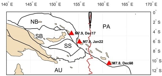
Figure 16. Pearson correlation coefficients of Swarm A/B/C Ne PSD with cumulative sum of seismic energy (black), ap (green), Dst (orange), and F10.7 (red), respectively (a) directly between daily Swarm Ne PSDs, cumulative sum for the short period of 5 days, ap, Dst, and F10.7, (b) using 5-day moving averages of all series except F10.7 (original daily F10.7 is used due to its apparent long-term character), (c) 7-day averages of all with original F10.7, and (d) 10-day averages of all with original F10.7. N and D denote nighttime and daytime tracks, respectively. The wavelength of Ne signal sampling is also given in km.

9. Conclusions

The preliminary observations of the common spectral patterns of ionospheric disturbances are promising for the future spectral recognition of short, along-track disturbed signals. Therefore, this study suggests that continuous tracking of seismic activity from the satellite orbit and spectral analysis of LEO along-track signals are fundamental and can facilitate the division of disturbed signals of different kind, e.g., distinguish preseismic from co-seismic ones. This also suggests that the processing of ground GNSS observations for LAIC studies should also use spectral analysis and must be considered not only at the time and place of the strongest earthquakes.

The visual observation of the correlations between Swarm Ne disturbances, seismicity, ap index, Dst index, and solar radio flux in Figure 7, Figure 8, Figure 9, Figure 10, Figure 11, Figure 12, Figure 13, Figure 14 and Figure 15 has been summarized by PCCs, calculated between Swarm Ne PSDs from three Swarm satellites and four remaining quantities: the cumulative sum of seismic energy, ap and Dst indices, and F10.7. The PCCs that were determined for the original data series (except seismicity, for which the shortest-term 5-day sum is used) are notable (≥0.3) only in three nighttime cases, but even these cases confirm the best correlation of the Swarm–seismicity pair. The 5-day averaging of all data series (except F10.7 due to its smooth long-term character in daily series) leads to a slight increase in correlations while still maintaining an advantage of Swarm–seismicity pairs. The increase of the averaging window to 7 days confirms the dominant correlation between Swarm Ne PSDs and weekly seismic energy, with the PCC reaching or exceeding 0.3–0.4 in all nighttime cases. At the same time, no significant increase in the PCC for the other data pairs is attained after 7-day averaging of the analyzed series. The averaging with a 10-day window increases all nighttime correlations of Swarm–seismicity pairs to 0.4–0.7, whereas the other pairs infrequently obtain an PCC equal to at most 0.3. These numbers strongly suggest that longer-term (several day) disturbances in Ne at a 300 km wavelength, recorded by Swarm 450 km over the tectonic plate boundary, are correlated predominantly with seismicity. Moreover, the correlation of seismicity with nighttime Ne variations is strong even without the determination of the respective time shift between these two phenomena. This can suggest that taking into account the time shift resulting from, e.g., the precursory character of Ne disturbances, can provide an even larger PCC. The first rough conclusion from the analysis of daytime Swarm LP observations is that the daytime LP Ne signal is less sensitive to ionospheric disturbances from the lithosphere at a 300 km wavelength. However, high PCC values at an 80 km wavelength in Papua New Guinea in the winter and spring support the suspicion that by analyzing very high frequencies, we can detect LAIC from the Swarm orbit, also in the daytime.

The long-term disturbances approximated by 7- and 10-day moving medians of the Swarm Ne PSD reveal a notably better correlation with persisting long-term seismic activity than individual Ne signal disturbances with individual large earthquakes. The persisting Swarm Ne disturbances often precede significant seismic activity, which can point to their precursory character. However, there are also many examples of disturbances occurring just after shallow earthquakes, at the end of an earthquake series, or in the middle of the series, which proves that this analysis over a longer time span is relevant, whereas a selective approach to seismicity studied with respect to LAIC can hide some important information.