Abstract
Reliable and accurate land-use/land cover maps are vital for monitoring and mitigating urbanization impacts. This necessitates evaluating machine learning simulations and incorporating valuable insights. We used four primary models, logistic regression (LR), support vector machine, random decision forests, and artificial neural network (ANN), to simulate land cover maps for Tsukuba City, Japan. We incorporated an auxiliary input that used multinomial logistic regression to enhance the ANN and obtained a fifth model (ANN was run twice, with and without the new input). Additionally, we developed a sixth simulation by integrating the predictions of ANN and LR using a fuzzy overlay, wherein ANN had an additional new input alongside driving forces. This study employed six models, using classified maps with three different resolutions: the first involved 15 m (ASTER) covering a study area of 114.8 km2, for the second and third, 5 and 0.5 m (derived from WorldView-2 and GeoEye-1) covering a study area of 14.8 km2, and the models were then evaluated. Due to a synergistic effect, the sixth simulation demonstrated the highest kappa in all data, 86.39%, 72.65%, and 70.65%, respectively. The results indicate that stand-alone machine learning-based simulations achieved satisfactory accuracy, and minimalistic approaches can be employed to improve their performance.
1. Introduction
Amid the escalating focus on global environmental change, carbon cycling levels, and sustainability, land change science has arisen as a specific scientific field dedicated to grappling with these complex phenomena [1]. The conversion of urban land use represents a tangible consequence of urbanization, which globally constitutes the second most significant source of greenhouse gas emissions [2,3]. Since it is considered the powerful propulsion of transformation in ecosystem function, one of the most critical ways to challenge the status quo in climate change and biodiversity loss is to quantify urban land dynamics [2,3]. Simulation of land changes underpins a baseline thematic map for natural resource management, environmental assessment, urban planning, monitoring, and designing sustainable ecosystem services [4,5,6].
In the past decades, the synthesis of art, science, and technology in detecting and classifying objects on Earth culminated in remote sensing. Afterward, geosciences and computer science intersections guided the development of geographic information systems (GIS) [7]. GIS provides a platform for managing, analyzing, and visually presenting spatial data in layered maps, thereby improving data comprehension and supporting more precise, efficient decision making in a single interface. Satellite remote sensing also enables synoptic measurements of the worldwide terrestrial surface across various spectral, spatial, and temporal resolutions [1,8]. Continuous advancements in GIS and sensor technology have profoundly augmented our capability to map urbanized regions, permitting accurate extraction of essential land cover categories, which holds substantial significance for global land change studies [9].
Scholars have undertaken serious attempts toward the modeling of land-use prediction [5]. Limitations in traditional approaches, like inflexible decision rules and limited representation of uncertainty, and given that urbanization is a multifaceted process influenced by various driving factors, have led them to look for more advanced modeling approaches [10,11].
When it comes to predictive capability and adaptability, machine learning is taking the simulation of urban growth characteristics to a whole new level in terms of operation [12,13]. This led to exponential growth in applying the machine learning-based algorithms individually or integrated with the Markov chain (MC) or cellular automaton (CA) [14]. Statistical/machine-learning techniques embody methods for delineating mathematical relationships between inputs (i.e., driving variables such as topographic slope and road proximity) and outputs (i.e., land-use/land cover (LULC) changes) [15]. The collected data are employed to create transition potential maps (TPM), which provide an empirically derived metric for assessing the likelihood of specific land transitions [15,16]. Several learning-based algorithms have been utilized to create the TPM, which encompass but are not restricted to support vector machine (SVM) [17], logistic regression (LR) [18], weighted normalized likelihood (WNL) [19], random forest (RF) [20], and artificial neural networks (ANN) [21]. One must acknowledge that, despite the rising prominence and accuracy of deep learning, traditional machine learning methods often provide greater transparency, interpretability, and computational efficiency. They also exhibit increased resilience against overfitting, particularly when faced with limited labeled data, and benefit from quicker training times and simpler architectures, which can minimize potential errors [22].
There is abundant literature on this field, emphasizing their positive performance and providing detailed information regarding their predictive potency upon review.
For instance, Arsanjani et al. [23] applied a hybrid model that combined LR, MC, and CA and demonstrated an 89% match between simulated and actual land-use maps for Tehran, validating its successful calibration and predictive capabilities for urban sprawl in future years. Moreover, several authors have recognized that, generally, LR presents interpretable results, well-organized missing or unbalanced data, provides probability estimates, showcases efficient training, and exhibits a lower propensity for overfitting [24,25,26,27]. In their study on enhancing a CA with SVM for urban growth modeling, Rienow et al. [28] found that SVM-based TPMs exhibit a high certainty. Their basic approach is to map samples as vectors in a high-dimensional space and classify them by maximizing the margin between support vectors and the hyperplane. Consequently, it is less interpretable but favored for its adaptability to complex datasets and nonlinear solid modeling capabilities [29]. Gounaridis et al. [30] applied a random forest-cellular automaton modeling approach to research future LULC change in Attica (Greece) under different socioeconomic realities and scales. Their results showed that the RF model was accurate in allocating the LULC change patterns within the study area, exhibiting a notably high overall accuracy of 88.36%.
Most early studies, as well as current work, in machine learning-based land transformation modeling focus on ANNs [31,32,33]. Neural networks establish representations of the correlations between land transitions and their associated variables by deploying a network of weighted connections, which the algorithm iteratively optimizes. Zhang et al. [34] employed the artificial neural network-cellular automaton-Markov (ANN-CA-Markov) model to simulate urban sprawl in China. Their findings revealed a suitability score of 0.864 for the ANN model, underscoring its efficacy in simulating urban sprawl. Moreover, with a kappa coefficient of 0.78, the ANN-CA-Markov model demonstrated high accuracy in urban sprawl simulation. In another study, Roy et al. [35] utilized spatio-temporal analysis and cellular automaton simulations of biophysical indicators under climate change and urbanization scenarios, employing an ANN. They achieved an 84% accuracy rate in LULC from the simulation metrics.
In another recent publication, Cuellar et al. utilized high-resolution WorldView-2 satellite images to model the complex dynamics in urban land change up to 2034 in Bogota using the MC, future land use simulation (FLUS), and ANN methods. Validation confirmed a machine learning accuracy with an average value of 0.85 [36].
It is noteworthy to mention that numerous studies have compared land change modeling approaches previously used in separate case studies. Consequently, the specific application of these models gives their conclusions a comparative bias [37]. Building on existing knowledge, each model utilizes distinct mechanisms to capture the correlation between land-use change and its underlying driving forces; hence, diverse simulated maps and prediction accuracies originate from the model’s assumptions, which necessitates further comparative analysis. In this relatively understudied topic, Shafizadeh-Moghadam et al. [37] conducted a comparative study of different models, including ANN, SVR, RF, decision tree (DT), LR, and multivariate adaptive regression splines (MARS), assessing their predictive accuracy in urban growth simulation. The study indicated the area under the curve (AUC) ranging from 67.6% (LR) to 74.7% (ANN), with substantial pattern disparities in spatial error maps.
However, to the best of our current understanding, there has yet to be comprehensive research that has simultaneously evaluated the principal machine learning-based urban growth prediction techniques through an identical region (in two different sizes) and with diverse satellite imagery across various temporal periods to compare their effectiveness. In addition, under this circumstance, the critical capability of combining two machine learning simulations compared to standalone ones has yet to be fully understood. The gap in the literature confronts us with limitations such as a lack of comprehensive understanding of different prediction techniques, reduced applicability of the findings, an inability to generalize results, and a lack of robustness in predictions.
Against the above background, this research aims to assess machine learning methods in the simulation of urban growth in Tsukuba, Japan, using three different resolution land cover maps spanning two different sizes and timeframes. Further, we intend to create and add a new input to the ANN-MC model and use this enhanced model to synergize with an LR-MC model through fuzzy logic. The ultimate objective is to scrutinize these six models, SVM-MC, random decision forests (DF)-MC, LR-MC, and two ANN-MC (once with and once without new input), alongside a hybrid model combining ANN-MC and LR-MC for their spatial accuracy and predictive capabilities. Our research intends to overcome existing limitations and would be a significant step toward enhancing the effectiveness and reliability of machine learning-derived urban growth predictions.
2. Materials and Methods
2.1. Study Area
The study area focused on in this research is Tsukuba City, situated in Ibaraki Prefecture, Japan. In Japan, most urban areas have matured, save for major redevelopments following significant disasters. However, Tsukuba stands out, showcasing urban expansion. The location of the study area is illustrated in Figure 1. This city, covering an area of 283.72 square kilometers, witnessed a growth in its population by 26,435 between 2005 and 2015 and further sustained a steady annual increase of 1.3% from 2015 through 2020. Situated along the Tsuchiura River, with a delightful climate and fertile soil, it provides an ideal environment for settlement. Tsukuba City, renowned as “Science City”, is well-connected via multiple train stations on the Tsukuba Express Line, a new railroad line that opened in 2005, enabling easy access to Tokyo [38]. This urban development and transportation efficiency attract an educated populace and foster substantial growth. The targeted area for analysis lies within the geographical coordinates 36.6°N and 35.58°N in latitude and 140.01°E and 140.07°E in longitude, reflecting Tsukuba City’s unique positioning in the context of urban growth and scientific advancement.
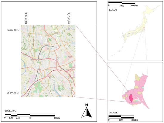
Figure 1.
Location of the study area.
2.2. Datasets
For historical data about the urban footprint, we utilized remotely sensed ASTER data satellite images taken between 2003 and 2012, which were captured in August 2003 and 2012. The employed images offer a spatial resolution of 15 × 15 m, effectively facilitating the classification of the LULC map during the specified period. Furthermore, this study incorporated high-definition imagery resources such as Maxar’s WorldView-2 and the GeoEye-1. The WorldView-2 imagery, exhibiting a spatial resolution of 0.46 m, was collected on 8 May 2010. Subsequently, the GeoEye-1 imagery, demonstrating a superior spatial resolution of 0.41 m, was captured on 1 April 2015. Utilizing these data sources enabled a more granular comparison of the subject matter.
The JAXA high-resolution LULC map product was the dataset used as ground truth [39]. This map was created using a convolutional neural network (CNN) algorithm for pattern recognition in multispectral and time series feature spaces. It was made using multiple datasets, including (1) Sentinel-2 Level-1C from Google Earth Engine API, (2) ALOS-2/PALSAR-2 data, (3) 25,000 training data points from the SACLAJ database including ground surveys and online interpretations, (4) ALOS PRISM Digital Surface Model, (5) a raster map of slopes from the digital surface model, (6) a vegetation survey map by the Biodiversity Center for interpreting bamboo forests, (7) data on photovoltaic power plants from Electrical Japan for interpreting solar cell panels, (8) coastline data from the Geospatial Information Authority of Japan, and (9) OpenStreetMap’s road network data for creating raster maps of distances from roads. We used the same data source for the road map as well.
We also utilized two distinct digital elevation models (DEMs) as part of our datasets. The first DEM was sourced from Earthdata, a NASA initiative, with a spatial resolution of 30 m [40]. The second DEM was procured from the Geospatial Information Authority of Japan (GSI), featuring a more detailed spatial resolution of 5 m [41]. In addition, the spatial population distribution datasets utilized in this study were sourced from WorldPop, a project affiliated with the School of Geography and Environmental Science at the University of Southampton [42].
2.3. Methodology
2.3.1. Overview
The methodology adopted in this study comprises a structured three-data process. The initial phase involves the supervised classification of pixels in raster datasets. Medium-resolution data from ASTER at 15 m were obtained for 2003 and 2012, and high-resolution data from WorldView-2 for 2010 and GeoEye-1 for 2015 at 0.5 m were classified. Additionally, cells of 5 m were extracted from the high-resolution datasets. This process resulted in the creation of three spatial resolution maps: one with 15 m resolution covering the period 2003–2012, another with 5 m resolution, and a third with 0.5 m resolution, both covering the period 2010–2015. In the second phase, the focus was on preparing explanatory variables, including DEM, slope, distance to urban areas, distance to roads, and spatial distribution of population. Additionally, efforts were made to improve the accuracy of the ANN model by introducing a new input to enrich the existing data pool. In the third phase, we simulated urban growth in Tsukuba, Japan, for the years 2020 and 2022. Medium-resolution data were utilized for the 2020 simulation, whereas high-resolution data were employed for the 2022 projection. Four distinct simulation models were used for this purpose: the SVM, DF, LR, and ANN-MCs. The ANN model was run twice—once with the new input data and once without them. Subsequently, the improved ANN-MC was integrated with LR-MC simulation through fuzzy logic techniques.
In the third phase, the final objective of the study was to evaluate and contrast the spatial accuracy and predictive power of these six methods. To validate the 2020 prediction, the ground truth data were sourced from the JAXA LULC map with a spatial resolution of 10 m. For the 2022 prediction validation, Google Earth was employed as the ground truth. A visual representation of the entire methodological sequence can be found in Figure 2.
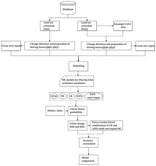
Figure 2.
Flowchart showing the LULC simulation and evaluation process for the six models.
2.3.2. Land Cover Classification and Ancillary Data Preparation
In the study, LULC classification was executed using ArcGIS Pro version 10.8.2 software, deploying a classification scheme featuring seven distinctive land-use categories. These encompass water, urban land, rice paddy, cropland, grassland, trees, and barren land. The classification was performed on satellite data employing a SVM supervised classification method, a methodology frequently adopted within the scientific research community.
After the initial classification, corrections were implemented for erroneous pixels within the generated LULC maps. Based on ASTER and Maxar data, the resultant classified maps covered areas of 114.8 km2 and 14.8 km2, respectively. Furthermore, classification maps of 5 m resolution were derived from the Maxar data-based maps through resample tool in Arc GIS Pro, which changes the spatial resolution of a raster dataset and sets rules for aggregating or interpolating values across the new pixel sizes. The extent of the raster dataset will remain the same.
The factors, also known as explanatory variables or drivers, that contribute to alterations in LULC are chosen based on their potential to augment or reduce the suitability of a particular option for the intended activity [43]. Typically, topographic elements like the slope and the DEM are seen as the most critical in influencing urban expansion. Other proximity variables, like the distance from developed areas and the proximity to roads, are also significant contributors to urban sprawl [44,45]. The principle of neighborhood effects typically indicates that undeveloped land surrounded by built-up areas is more likely to become a developed area eventually [46]. Accordingly, other ancillary data inputs were prepared, including the DEM, slope (derived from DEM), the spatial distribution of population, distance from the road, and distance from the built-up area.
Also, given that GSI provides 5 m DEM XML files [41], we utilized the QuickDEM4JP tool within the QGIS 3.26 software to convert these files into a more user-friendly DEM Geo Tiff format. It is worth noting that these ancillary data were extracted at three different resolutions, like the classification maps, providing a spectrum of granularity for future modeling and analysis.
2.3.3. New Auxiliary Input for ANN-Multi Layer Perceptron
The variables play a key role in facilitating the solution of complex nonlinearities by ANN-multi layer perceptron (MLP) and enhancing accuracy [47,48]. In the field of predicting urban expansion, the range of input data is confined explicitly to specific parameters such as topographical characteristics, accessibility considerations, and demographic factors. One of the few attempts to use a helpful input besides these parameters is using evidence likelihood transformation in the analysis [49]. The information that may be helpful in training MLP both independently and in interaction with other variables. The bedrock of our strategy is built precisely upon this foundation. Incorporating a version of the new input data that contain some useful patterns in the ANN-MLP framework allows for a more comprehensive understanding of the interplay between various land uses and the probability of their conversion into urban areas. To accomplish this, first, we extract the change maps, which represent the pixels transitioned to urban land, for example, “forest pixels to urban”, “cropland pixels to urban”, and “barren pixels to urban”. In fact, this multi-categories map consists of changed pixels and their land-use origins before conversion into urban land use. Second, we apply multinomial logistic regression (MLR), wherein the change maps as dependent variables and driver forces serve as independent variables within the model.
MLR tries to model the relationship between one dependent variable and independent variables. The model does this by calculating log odds, also called logits, and these logits are then transformed into probabilities. Therefore, the output of this model would be a set of probability maps, which shows the predicted probability that a land-use class has changed to an urban, given the values of the independent variables at that location. As an exquisite statistical method, MLR lends itself to GIS, and due to adept management of multiple-category dependent variables, without requiring assumptions such as linearity, homoscedasticity, or normally distributed errors, along with its capacity to offer insights into the effect size through odds ratios, has been gradually popularized as a user-friendly geospatial modeling technique [50,51].
The logit (𝓁ij) represents the logarithmic function of the odds of a pixel (i) belonging to a class (j). The predictor values can be used to predict its value using a regression function derived from directly:
𝓁ij = ln (Pij/(1 − Pij)) = β0 + β1jx1i + β2jx2i + … + βnjxni
Thus, given the independent variable vector X, the conditional probabilities of each outcome category can be calculated by the following formula [52]:
MLR utilizes the maximum likelihood estimation (MLE) approach to identify the most optimal set of parameters, also known as coefficients. In essence, MLR serves as a maximum entropy solution, as it actively seeks the parameters that best fit the data [53]. We employ the statistical tool provided by the TerrSet IDRISI 2020 software for this purpose.
To sum up, the modeling of ANN-MLP is based on samples of pixels that underwent the transition and samples that could have undergone it but did not. Therefore, the spatially detailed view of how historical land change data are associated with change agents helps ANN-MLP better understand the distribution of these changes across the landscape. Because ANN-MLP is mighty in modeling interactions through its hidden layer, theoretically, by adding an auxiliary input with meaningful information, the model can understand and use it.
2.3.4. Transition Potential Modeling and Markov Change Model
The transition potential provides invaluable insights into the spatial distribution and potential of future changes [54]. It can be operationalized in the context of land cover changes, where different transitions could be classified under specific sub-models, given that the drivers causing such changes remain consistent across each transition [55]. To provide an example, the factors that contribute to the conversion of forest lands into urbanized areas may be the same as those that drive the transformation of forests into croplands. As a result, changes in LULC influenced by these common variables are combined and analyzed within specific sub-models [56].
In addition, the polynomial trend surface, which can capture and streamline complex spatial trends in data, was selected to facilitate interpretation and predict spatially related outcomes, like transition potentials. The models used in this research consist of: ANN-MLP, SVM, DF, and LR within the TerrSet IDRISI software.
- (1)
- ANN-MLP
The MLP neural network, a subtype of feedforward neural networks, comprises three core layers: input, hidden, and output layers. Its operation hinges on the supervised backpropagation (BP) algorithm, a cornerstone of land change modeling [57]. The MLP employs feedforward algorithms to assign weights to input values, and nodes across the three layers, which are then propagated via the hidden layer, a compilation of computational nodes, to the output layers. The MLP can facilitate multiple transitions concurrently during the modeling process [58,59]. Data flow within the MLP is unidirectional, progressing from the input layer through the hidden layers to the output layer. This structure enables the MLP to establish non-linear relationships within the dataset. Within these layers, nodes are organized in such a way that each node accepts an input signal from various nodes, applies a transformation, and then transmits the altered signal to subsequent nodes. Each originating input layer node is assigned a weight inclusive of a threshold and is subsequently processed through either a linear or non-linear activation function. They can be expressed as follows [21]:
The spatial variables are given by:
where is the i-th attribute, and T is transposition.
Neuron j in the receiver layer, the Z input from the collection process is calculated by:
where is the weight between the input and the hidden layers, and is the i-th scaled attribute associated with the i-th neuron in the input layer with respect to the c-th cell at time t.
The activation of the hidden layer to the input signal is calculated by:
The following formula calculates the transition probabilities according to the output function of neural networks:
where p (k,t,l) is the probability of transition from the existing to the l-th type of LULC for the c-th cell at time t, and is the weight between the hidden and the output layers.
The training process, which aims to minimize the discrepancy between observed and anticipated outcomes, requires fine tuning these weights before the system can be operational for forecasting purposes [58]. Once the MLP has undergone training, incorporating many influencing factors for each sub-model, it generates time-explicit transition potential maps. These maps illustrate the time-explicit change potential, a valuable resource for understanding temporal dynamics [59].
- (2)
- SVM
In the context of land cover modeling, the process using SVM with the radial basis function (RBF) kernel begins with the input data. These data are then mapped to a high-dimensional space using the RBF kernel, adept at handling non-linear data intricacies. Essentially, the RBF kernel computes a similarity measure or “distance” between each pair of data points. Unlike a simple geometric distance, this measure encapsulates the complex, non-linear relationships among the features [60,61]. For variable evaluation, the SVM in TerrSet uses a backward stepwise constant forcing strategy, the same as ANN-MLP. The SVM module will start with all variables and then calculate the decreased 5-folded cross-validation accuracy by holding constant each variable in turn. The variable with the most decreased cross-validation accuracy will be taken as the most important variable. After completing the training of SVM and optimizing its parameters, the model is ready to be utilized for predicting future transition potential maps.
- (3)
- DF
With the data prepared, the DF algorithm starts building the forest, which is an ensemble of decision trees. Each tree is built on a bootstrapped subset of the data. For each node in the tree, a random subset of the predictors (input data) is selected, and the best split among these predictors is chosen based on a measure like the Gini impurity or information gain. This process continues until the tree is fully grown and replicated across multiple such trees forming the “forest” [62,63]. In the context of land cover modeling, each decision tree in the forest represents a possible sequence of land-use changes based on different combinations of the input variables. The randomness introduced by bagging and random feature selection ensures that each tree captures different aspects and complexities of the land-use transition process [20]. To make a prediction for a new data point, it is passed down to each tree in the forest, resulting in a series of predictions. The final prediction is typically the mode (for classification) or mean (for regression) of these individual predictions. This voting mechanism makes the model robust and less prone to overfitting. Importantly, DF also provides a way to assess variable importance. This is done by randomly shuffling each predictor’s values and measuring how much the prediction error increases. This helps understand the influence of different geographical features and human factors on land-use changes. The DF model can use this process to predict land-use transitions based on various environmental and anthropogenic factors.
- (4)
- LR
The binary LR model, a variant of the MLR, has proved to be an effective tool in modeling urban growth [64]. The cell-based nature LULC falls into two distinct categories: the presence or absence of urban growth. In binary logic, we can use the value 1 to signify urban development and 0 to denote the lack of urban growth. It is postulated that the probability of a cell transitioning to urban use follows a logistic curve as dictated by the logistic function [65]:
This premise leads us to the LR model, which allows us to estimate the likelihood of a cell undergoing urbanization. The formula can be represented as follows [25]:
In this equation, P (Y = 1|, , …,) symbolizes the probability of the dependent variable Y taking the value 1 given , , …,), essentially the likelihood of a cell becoming urbanized. Each Xi represents an independent variable that acts as a driving force of urbanization, capable of being of interval, ordinal, or categorical nature. Correspondingly, βi is the coefficient attached to variable Xi. This framework enables us to understand and predict the dichotomous behavior of cells in our land cover model, precisely the manifestation or lack of urban growth.
Once transition potential maps are generated, they get incorporated into an MC simulation. An MC is a stochastic process that provides a statistical framework for forecasting events in a sequence, where the probability of evolving into a subsequent state is reliant solely on the present state and not on the sequence of prior states. Upon the generation of transition potential maps, the MC model becomes instrumental for predictive applications. The Markov process quantitatively anticipates the precise extent of land that is projected to transition from the later date to the target prediction date based on the extrapolation of future transition potentials. It is imperative to underscore that this procedure does not equate to a rudimentary linear extrapolation, as the transition probabilities inherently exhibit dynamic behavior over time until they arrive at an equilibrium state.
2.3.5. Final Simulation for Tsukuba 2020 and Tsukuba 2022
After extracting transition potential maps, the transition probability matrix of an MC by defining a final date for prediction is calculated in TerrSet. This enabled us to simulate Tsukuba City for 2020 using a combination of machine learning models and MC, all with the ASTER data classification map. The simulation of 2022 will be conducted twice and over a smaller area. Once with a 5 m resolution, once with a 0.5 m resolution.
After completing these simulations, we import the results from the TerrSet 2020 software into ArcGIS Pro. We then designate these imported data as a conditional raster and a constant input value in the Con tool of the software. This allows us to execute a conditional if/else analysis on each cell of the input raster. The final stage of the process entails converting the analyzed raster into a classification map with seven categories.
2.3.6. Fuzzy Overlay
Fuzzy overlay analysis is a technique used in geographic information systems for spatial decision-making tasks [66]. It helps to determine the suitability or potential of different locations based on different criteria [67]. This method can be particularly beneficial for an exploratory location study where various criteria need to be evaluated to find the most suitable location [68].
In this study, we employ the fuzzy technique as an easily implementable, flexible method to develop a straightforward heuristic model for urban pixels. Indeed, the source maps selected for the fuzzy overlay approach in ArcGIS Pro are based on the machine learning-based simulators determining the most potential locations of urban areas. In doing so, upon completion of the simulation, the method of fuzzy overlay was employed to synthesize two sets of raster simulation maps generated by the ANN-MC (which utilized novel input) and the LR-MC. The Gaussian function was hired to fuzzify the criteria. Since the aim was for optimal prediction and distribution of urban (second class) pixels, the fuzzy AND type was selected as an intersection operator for this purpose. The Gaussian function, with a spread value of 0.1, was used for the fuzzy overlay membership, and the software determines its midpoint based on the range of input raster values. Applying the fuzzy overlay essentially aggregates the predictions from both models, allowing for a more nuanced prediction.
Given its foundation and purpose, we have aptly named this new approach the ‘neural logistic fuzzy ensemble method’ (NLFEM).
2.3.7. Validation of Simulation Models
We assessed the performance of six predictive models across all three data using a comprehensive set of metrics suitable for land-use change simulation science. These metrics, including kappa coefficients for categorical assessments and sensitivity, specificity, precision, accuracy, F1 score, Matthew’s correlation coefficient (MCC), and receiver operating characteristic (ROC) for binary accuracy assessments within urban pixels, allow for a detailed evaluation of each model’s effectiveness.
To provide some insight, the kappa coefficient, which is based on the confusion matrix often used to measure the agreement between predicted and observed categorizations, is employed, with a higher value indicating better performance [69,70].
where r: number of rows in the error matrix,
: the number of observations in row i and column i (on the major diagonal),
: total of observations in row i,
: total of observations in column i,
N: total number of observations included in matrix.
The binary metrics focus on urban pixels. Sensitivity (also known as the true positive rate) measures the proportion of actual positives that are correctly identified. In contrast, specificity (true negative rate) measures the proportion of actual negatives that are correctly identified [71].
where TP represents the true positive, FN represents the false negative, TN represents the true negative, FP represents the false positive.
Sensitivity = TP/(TP + FN)
Specificity = TN/(FP + TN)
Precision, synonymous with the positive predictive value, along with accuracy, indicates the overall trustworthiness of the predictions. A higher precision and accuracy suggest a reduced occurrence of both false positives (non-urban areas incorrectly identified as urban) and false negatives (urban areas inaccurately identified as non-urban) [72].
Precision = TP/(TP + FP)
Accuracy = (TP + TN)/(TP + TN) + FP + FN
In assessing land-use simulation accuracy, F1 score [73] and Matthew’s correlation coefficient (MCC) [74] offer distinct advantages that complement traditional accuracy metrics. The F1 score, a harmonic mean of precision and recall, provides a balanced measure of the model’s performance, particularly in situations with uneven class distributions [73]. It ensures that both the model’s precision (how many selected instances are relevant) and recall (how many pertinent examples are chosen) are considered, thereby reducing the potential bias towards overrepresented classes. On the other hand, the MCC provides a robust evaluation metric for binary classifications, offering a more reliable statistical rate of true and false positives and negatives [74]. Unlike different coefficients, MCC considers all four values of the confusion matrix, giving a balanced measure even in imbalanced class distribution. Hence, using these metrics together can help develop a more holistic understanding of a model’s performance across different land-use categories, considering both the balance between precision and recall and the true rate of correct and incorrect classifications.
F1 Score = 2TP/(2TP + FP + FN)
MCC = (TP × TN − FP × *FN)/sqrt ((TP + FP) × (TP + FN) × (TN + FP) × (TN + FN))
The receiver operating characteristic (ROC) curve, alongside its related part, the area under the curve (AUC), serves as a robust measure for assessing the efficacy of the predictive model. These analytical tools were utilized to evaluate the model’s proficiency in accurately distinguishing between binary categories, specifically urban and non-urban classifications [75]. The ROC and AUC furnish a quantifiable means to gauge the accuracy and discriminative capacity of each predictor, thereby facilitating the identification and prioritization of the most consequential predictors.
3. Results
3.1. Land Cover Change Analysis
The LULC maps, derived from ASTER data for the years 2003 and 2012 spanning areas of 114.8 km2, and Maxar data for the years 2010 and 2015 covering areas of 14.8 km2, are displayed in Figure 3. As previously elucidated, a five-meter resolution land-use classification map was extracted from the Maxar 0.5 m data to facilitate the performance assessment of urban growth predictors, focusing on three distinct spatial resolutions.
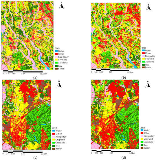
Figure 3.
Land cover classification maps. (a) ASTER-based classification map 2003; (b) ASTER-based classification 2012, (c) WorldView-2-based classification 2010, (d) GeoEye-1-based classification 2015.
The outcome of the change analysis reveals a notable expansion in urban land cover. Specifically, between 2003 and 2012, the urban area experienced an augmentation of 9.49 km2. This increase was fueled by the transition of different land cover types to urban areas, including 3.57 km2 from rice paddy fields, 2.45 km2 from cropland, 1.04 km2 from tree-covered places, 0.46 km2 from barren lands, and 0.546 km2 from grasslands. Furthermore, between 2010 and 2015, the urban space extended by an additional 1.53 km2. This expansion comprised 0.49 km2 from cropland, 0.21 km2 from barren lands, and 0.16 km2 from forested areas. The spatial trend of changes is illustrated in Figure 4.
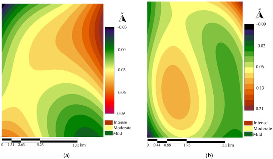
Figure 4.
Spatial trend surface (third-order trend) of LULC dynamics. (a) The trend of change from all classes to urban areas between 2003 and 2012. (b) The trend of change from all classes to urban areas between 2010 and 2015.
3.2. The New Input for ANN-MLP
The predominant transitions, as well as the pixel change maps, can be efficiently extracted from the change analysis tab of the TerrSet IDRISI software suite. These identified transitioned pixels from 2003 to 2012 and from 2010 to 2015 are specified as dependent variables. At the same time, the spatial trend of change, DEM, slope, the spatial distribution of population, proximity to roads, and distance to urban areas are designated as independent variables for the MLR tool. The default settings of the MLR tool are generally suitable. The software generates results for each category of the dependent variables and provides them in the results tab individually.
Figure 5 illustrates the outputs of MLR, which are considered probabilities maps and are different from TPMs. The MLR function modeled how the previous land-use status, before being converted to urban land, was influenced by a specific driving force, and produced logits. These logits were subsequently transformed into probabilities. These maps offer precise spatial information illustrating how spatial factors influence urban expansion, specifically about proximity to built-up areas. Additionally, they display clear patterns of road networks and well-defined outlines of railroads. In other words, they are an already-interpreted version of the original data, which can potentially augment the ability of ANN-MLP to pinpoint the pixel with a high propensity to transition.
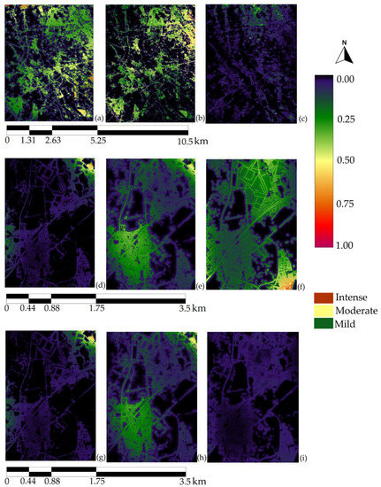
Figure 5.
MLR outputs: (a) from cropland to urban in ASTER data; (b) from rice paddy to urban in ASTER data; (c) from trees to urban in ASTER data; (d) from barren to urban in Maxar data (5 m); (e) from cropland to urban in Maxar data (5 m); (f) from trees to urban in Maxar data (5 m), (g) from barren to urban in Maxar data (0.5 m); (h) from cropland to urban in Maxar data (0.5 m); (i) from trees to urban in Maxar data (0.5 m).
Assessing the correlation among independent variables is crucial in regression analysis, where the variance inflation factor serves as a vital measure of multicollinearity. This factor exceeding 10 typically signifies a multicollinearity issue [76]. Since the factor for all the explanatory variables was calculated to be one, it suggests the absence of multicollinearity among these variables. This indicates that these predictors are relatively independent, each providing unique and valuable information to the model.
3.3. Accuracy Rate and Skill Measure of ANN-MLP
The skill measure and accuracy rate for each of the two ANN-MLPs are detailed in Table 1. The skill measure leverages Time 1 and Time 2 land cover maps, contrasting the number of correct predictions, after subtracting those due to chance, with a theoretically ideal set of predictions [77]. It is important to note that the skill measure does not project the model’s future performance; it is a tool for assessing how effectively the explanatory variables accounted for the historical changes. The accuracy rate and the skill measure indicate significant variability in the confidence levels for different transition predictions made by the model. Given that the ANN-MLP was run twice to create possible transition maps—once including new auxiliary inputs and once without—a comparative analysis was conducted to understand the performance of these two sub-models.

Table 1.
Performance indicators of two ANN-MLPs in all three data. Numbers in bold indicate the better values between the two ANN-MLPs.
In the initial phase of the simulation, premised on ASTER-derived data, a notable enhancement was observed in the accuracy assessment and skill measure for the ANN-MLP with the addition of additional input. More specifically, these parameters exhibited an increase of 28.5% and 28.3%, respectively, when contrasted with the ANN that operated without the new input. However, the second phase of the simulation, grounded in Maxar data with a spatial resolution of 0.5 m, failed to manifest a substantial augmentation. Notably, the accuracy assessment and skill measure demonstrated nominal growth, which increased by 0.68% and 0.93%. As the simulation advanced into its third phase, predicated on 5 m data, these performance metrics reported an uptick, rising by 9.6% and 14.2% in the same order.
3.4. Transition Potential Map
The exceptional features of high-quality transition potential maps can be summarized as follows: a distinct demarcation between cells with high and low potential, precise recognition of gradients that indicate gradual transitions, identification of hotspots representing areas with significant transition potential, and effective handling of sparsity [78]. In this section, we explore the analysis of the TPM maps, taking into consideration these specific characteristics.
Upon completion of the training and evaluation phases, five models, namely (SVM, DF, LR, ANN, and ANN with new input), were used to project TPMs for two different expanses of the Tsukuba study region, provided in three varying resolutions. The TPMs generated by these models are illustrated in Figure 6. For the period spanning from 2003 to 2012 within this region, the majority of land transitions were classified into three primary categories: from rice paddies to urban, from croplands to urban areas, and from forestlands (trees) to urban areas. Later, between 2010 and 2015, the primary transitions observed were from barren lands to urban, along with the sustained change from croplands and forestlands to urban regions.
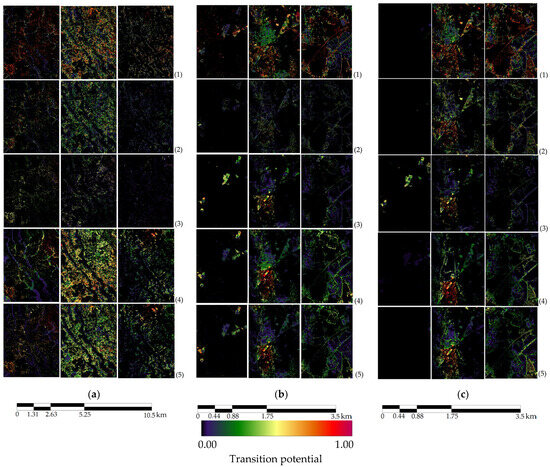
Figure 6.
Transition potential maps of Tsukuba projected by (1) SVM, (2) DF, (3) LR, (4) ANN, and (5) ANN plus with new input. (a) Implementing the algorithms utilizing ASTER data, (b) implementing the algorithms utilizing 5 m Maxar data, (c) implementing the algorithms utilizing 0.5 m Maxar data.
During the usage of the ASTER image-based classification maps, the SVM model demonstrated good sparsity and inclusivity, covering regions with high and low potential cells throughout the area under consideration. Moreover, distinct transition patterns are apparent in both ANN-MLP models as well; that is, they provide unique and clear differentiations between land-use classes and their related transition potentials in their predictions. Moreover, these models established a clear boundary between high- and low-potential cells within each of their maps, suggesting that they have successfully learned to differentiate urban growth features from non-urban growth features.
Regarding using 5 m resolution maps, the LR and both ANN-MLP models exhibited distinctive patterns in their predictions for the transition categories. Moreover, regarding spatial detail, gradient quality, and even the sparsity of TPMs, both ANN-MLPs surpassed the other models. It is worth noting that the ANN-based TPMs did not display any numerous dense clusters of high-potential cells scattered across different regions, thereby suggesting the absence of model overfitting.
Using 0.5 m resolution maps, the LR model effectively depicted the transition potential from barren to urban lands, accurately portraying the gradients and hotspots of these potentialities. The TPMs predicted by the DF and SVM models were analogous, whereas the ANN model with the new input data generated a more discernible separation between high potential and low potential regions at a broad scale than the ANN model just with standard driving forces. These attributes suggest that the ANN-MLP (with the new input data) proficiently learned the driving mechanisms of underlying urban growth.
3.5. Final Simulations
By comparing the LULC maps of 2012 and JAXA 2020, it is evident that the urban pixel count has risen from 73,000 to 113,000. This number in machine learning-based prediction maps ranged between 93,000 and 96,000 urban pixels. Notably, when combining ANN and LR, the count of urban pixels reached 106,000, highlighting that, although there is overlap in the predicted pixels of urban growth between both models, there are instances where each model separately identifies distinct areas as urban pixels on the map.
From 2015 to 2022, the growth of urban areas was also evident, albeit on a smaller scale, and the combination of ANN and LR still showed complementary predictions in some areas. The resulting output of the combination is shown in Figure 7.
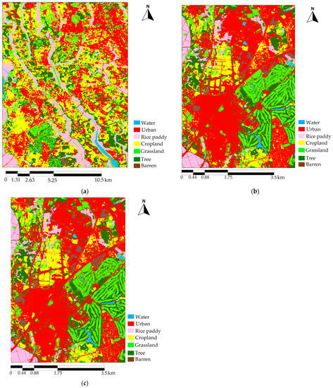
Figure 7.
LULC prediction maps simulated by NLFEM. (a) Prediction of urban growth in Tsukuba 2020 using ASTER data, (b) prediction of urban growth in Tsukuba 2022 using Maxar data (5 m), (c) prediction of urban growth in Tsukuba 2022 using Maxar data (0.5 m). The urban growth in Tsukuba during the mentioned periods was characterized by strategic land readjustment projects, the development of new urban areas around railway stations, and an increase in population. Central to this urban expansion was the Tsukuba Express Line, which not only enhanced connectivity but also served as a significant catalyst, steering the trajectory of the city’s urban development.
3.6. Accuracy Assessment
Multiple aspects were considered in the evaluation of the performance of six different simulations. These aspects include categorical metrics like kappa coefficients, as well as binary classification metrics such as sensitivity, specificity, precision, accuracy, F1 score, and Matthew’s correlation coefficient. The simulations were specifically focused on the classification of urban cells. Table 2 presents the accuracy levels achieved in six different simulations, while Table 3 provides the results of binary testing conducted on urban pixel analysis.
Table 2.
Kappa coefficients of the six prediction models for the three data. “+ANN-MC” indicates the ANN-MLP model with the new input data. Numbers in bold indicate the best values among the six models.
Table 3.
Binary testing results for urban pixels from the six prediction models. “+ANN-MC” indicates the ANN-MLP model with the new input data. Numbers in bold indicate the best values among the six models.
High resolution often means more variability, complexity, and heavy processing, which can result in models not generalizing well to new data. Furthermore, using a small area for training may not provide a diverse enough sample for the model to learn effectively. This lack of representativeness can lead to poorly performing models on unseen data, which diminishes kappa.
In prediction, urban growth with 15 m classification maps, the NLFEM and the ANN, which used new auxiliary input, are identical in precision and specificity, which means they perform similarly in correctly identifying true negatives (correctly predicted as non-urban) and avoiding false positives (incorrectly predicted as urban). However, the NLFEM has a better balance between precision and recall and classifies more instances correctly overall based on its value in F1 score and accuracy. Moreover, regardless of these two, LR performed better than the rest, so the effect of using LR and its combination through a fuzzy overlay with the reinforcement ANN appears here. In addition, a 4% increase in accuracy and F1 score between two ANNs represents the fact that additional input has valuable information, making ANN better at handling positive instances (correctly predicted urban and non-urban cells). The values of the F1 score and MCC for NLFEM were the highest, implying superior overall performance and quality urban cell classifications among the simulations examined.
In the subsequent phase, the expanse of the study area was reduced by a factor of eight. Moreover, the time gap between the two classification maps was shorter. These factors pose challenges to the machine learning models as the changes within such a brief period are relatively insignificant, while the smaller area makes it more arduous to identify patterns of change and predict cells with transmission potential. Additionally, the 5 m resolution provides excellent spatial clarity, but the increased number of pixels also lengthens the processing time. The ANN’s performance with the new input was nearly equivalent to that of NLFEM, and both models outperformed others in accurately simulating urban cells. The ongoing improvement in ANN’s accuracy, registering a 4% increase with the new input compared to its performance without it, shows that MLR-derived likelihood maps have continued to enrich the training of the ANN. In smaller areas, the spatial difference between the urban cells predicted by the models is less compared to the larger sites, so in this area, combining ANN with LR only resulted in a 1% increase in accuracy. Overall, the disparity in the accuracy of the machine learning models only reached a maximum of 5%, and they demonstrated commendable performance.
The third data remained identical in terms of both expanse and timeframe as compared to the previous step, though there was an enhancement in the map resolution to 0.5 m. The accuracy of every model declined, with the exceptions of enhanced ANN, whose performance remained stable, and SVM, which demonstrated an improvement. The precision of SVM surpassed that of NLFEM by 2%. However, when considering the harmonic mean of precision and recall, the NLFEM outperformed both by a margin of 1.6%. This was because of the higher value of SVM in the specificity and the higher value of NLFEM in the sensitivity.
Figure 8 displays the ROC curve, providing a visual depiction that effectively demonstrates the models’ ability to distinguish urban cells from non-urban ones. In two cases, the ANN outperformed other stand-alone ML models in AUC when utilizing the helpful and understandable relationships of land-use change as new input. Furthermore, the highest AUC across all cases was achieved when its final simulation was combined with the logistic simulation via a fuzzy overlay.
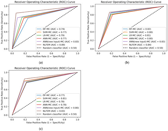
Figure 8.
Performance evaluation of models at three resolutions using ROC and AUC. (a) Using ASTER data, (b) using Maxar data (5 m), (c) using Maxar data (0.5 m).
4. Discussion
Our study aimed to improve the reliability and effectiveness of machine learning models used in predicting urban land growth. Four primary machine learning models—LR, SVM, DF, and ANN—were utilized to simulate the land cover map of Tsukuba, Japan. To enhance the generalization of the ANN, we incorporated an auxiliary input created by MLR. We ran ANN twice, with and without the new input, for improved comprehension, resulting in a fifth simulation model. Additionally, we created a combined model that merges the simulations of ANN (with the new input) and LR through a fuzzy overlay, producing a sixth simulation. These six simulation models were tested on three different classification map resolutions across two different sizes of the study area—one small and the other eight times larger. We evaluated the performance of the models using various metrics such as kappa coefficients, sensitivity, specificity, precision, accuracy, F1 score, and Matthew’s correlation coefficient specifically for urban pixels.
This study provides valuable insights into applying machine learning models in predicting urban growth patterns across different geographical scales and resolutions. Results showed that the range of discrepancy between the highest and lowest correct prediction, as indicated by the kappa coefficient for all stand-alone models, varied slightly across different data, at approximately 0.037, 0.036, and 0.034, respectively. These slight variations suggest that the models have almost similar levels of performance variation across different resolutions and areas. This implies that none of the models significantly outperforms or underperforms the others consistently. From a closer analysis, we observe that kappa values decline from the range of 0.774 to 0.812 in dataset with larger time differences to the range of 0.668 to 0.705 in the second dataset with shorter time differences. Therefore, the observed 10% performance decline might be ascribed to limited variation in the data resulting from the minor urban growth in two near periods with smaller study areas. Insufficient data diversity constrains model learning capacity, thereby impacting their ability to generalize across scenarios. Moreover, upgrading the resolution of classification maps significantly increased computational and processing demands, so that the production of TPM took a lot of time, and our findings show that elevating resolution from 5 m to 0.5 m resulted in a mean reduction of 1.5% in kappa and 3% in AUC across all models, except for SVM. This is possibly caused by SVM being more effective in high-dimensional spaces due to its ability to find optimal hyperplanes that separate data points accurately [79]. Our key findings also indicate that, by considering the past frequencies of transitions and their connections with the change factors, the ANN-MLP can more accurately reflect the dynamics of the land-use change. This rationale stems from the inherent workings of ANN and MLR mechanisms. MLR models the relationships between the type of land origin (historical transitions) and different change agents and creates maps that depict transition probabilities. ANN modeling is based on samples of pixels that underwent the transition and samples that could have undergone it but were not changed. Therefore, the transition likelihood map, with a spatially detailed view of how historical land change data are associated with change agents, helps ANN better understand the distribution of these changes across the landscape. Because ANN is mighty in modeling interactions through its hidden layer, the model can understand and use it by adding an auxiliary input with meaningful information. In detailing the performance advancements, the skill measure for ANN’s enhancements rose from 0.328 to 0.421 when simulating the 2020 LULC with a 15 m resolution. It further improved from 0.421 to 0.480 when modeling the 2022 LULC with a 5 m resolution and from 0.528 to 0.533 for the same year with 0.5 m data. Concurrently, the accuracy rates also saw marked growth, registering at 44.05% to 56.62%, 51.76% to 56.73%, and 60.69% to 61.10% across these scenarios, respectively. Correspondingly, the F1 score mirrored these improvements, registering increases from 78.4% to 82.4%, 79% to 82.7%, and 78.4% to 80.3% for each respective scenario. Additionally, to leverage the synergistic effects of machine learning predictions, ANN, for to its ability to solve complex non-linear problems [80], and LR, due to its efficiency with small datasets, robustness to outliers, and being less prone to overfitting [81], were chosen to combine. The fuzzy overlay results of these two models show an improvement in urban cell location in the final land-use simulation, which allows for a more nuanced analysis. The ability to differentiate urban cells from non-urban ones, measured by the AUC, reaches its highest levels in all three study cases: 0.89, 0.84, and 0.83. Likewise, its F1 score increased by 7.1%, 1.8%, and 2.4% compared to the second highest F1 score. It can be inferred that each of the ANN and LR models exhibits accurate urban pixel predictions for some different areas on the map, thereby demonstrating a complementary relationship that enhances overall performance when combined.
There is limited comparative research in urban growth utilizing machine learning models, and Bin Zhang et al. [78] represent one of the few notable studies in this area. Their study utilized land-use data from GlobeLand30 for the years 2000 and 2020. They employed LR-CA, ANN-CA, SVM-CA, and MaxEnt-CA models to simulate urban growth in Beijing, Tianjin, and Wuhan, and the performance of these models was evaluated based on various factors, including training, testing, projection accuracy, computational efficiency, simulation accuracy, and the simulated urban landscape. The disparity between the highest and lowest kappa values was 4.2, 3.4, and 5.9, respectively, slightly more than our results but still highlights the nearby degrees of performance variation. Moreover, ANN demonstrated superior computational efficiency by effectively learning and discerning distinctive class features, mirroring our research findings. In another study, Wang et al. [82] demonstrated promising outcomes by integrating historical data into a cellular automaton model to simulate the expansion of urban land. While their approach differed from the one employed in the present study, both investigations revealed the beneficial influence of incorporating historical transitions on enhancing accuracy. Furthermore, despite the increase in accuracy after adding the new input, ANN (without new input) still had the highest kappa compared to the SVM-MC, LR-MC, and DF-MC in the first step, with a larger area and more noticeable urban growth, while this was not the case in the smaller size. Therefore, our research corroborates previous studies indicating the ANN is a data hungry model; when the dataset is small or biased, the network might struggle to grasp the fundamental patterns and connections among the data points [83,84]. In Pir Mohammad et al.’s [85] research, a CA model based on ANN was employed to forecast future LULC, and the model achieved an overall accuracy of 89.2% which was higher than our results. This was while we were using the JAXA LULC map as the ground truth with a 10 m resolution which is higher than ASTER.
Our key methodological contributions enhance urban growth prediction accuracy, showcasing the adaptability of machine learning. The primary innovation is elaborating an underlying driver as a new input for ANN in urban dynamics modeling. This input unravels the spatial ties between historical data and change agents using MLR. Our findings reveal that the ANN forges interactions by effectively channeling this auxiliary information in its hidden layer. Quantitatively, the performance leaps in ANN’s accuracy rate and skill measure are notable and resonate with the F1 score’s upward trajectory. Additionally, the amalgamation of ANN and LR through fuzzy overlay shows their synergistic effectiveness in the outcomes. Our methods offer increased flexibility relative to current literature, setting a refined precedent for subsequent studies. These techniques are appropriate for cities undergoing land-use transformations and urban growth. They are adaptable to various urban patterns and can be generalized to different scales, making them relevant for most urbanized regions. However, despite this study’s valuable findings, certain limitations need to be addressed. Firstly, evaluating the four models has primarily focused on their effectiveness with MC models, and their ability to predict urban growth in a broader context accurately requires further investigation. Secondly, the impact of high-resolution data in a larger study area, where urban growth is more evident, may yield different results for the model’s performance. Therefore, conducting additional research to examine these influences more comprehensively is crucial. Lastly, while our approach in creating new input for ANN and fuzzy overlay-based combination of this ANN and LR shows promise in enhancing accuracy, its reliability should be further validated. Future analyses could apply these simulations to different regions to corroborate the findings of this study and ensure their generalizability.
5. Conclusions
This research study aimed to improve the reliability and effectiveness of machine learning models used in predicting urban land growth. Six simulation models, including LR, SVM, DF, and ANN, once with the new auxiliary input and once without, and lastly, a combined ANN and LR model through a fuzzy overlay, were evaluated and tested with three different classification map resolutions and two study area sizes.
The results show that the performance of the stand-alone machine learning models produced an acceptable level of accuracy, and the disparity between the highest and lowest levels of kappa varied slightly across different data. However, there was a kappa deterioration due to limited urban changes from 2010 to 2015 in smaller study areas. Therefore, area size and amount of urban change impact the models’ ability to generalize across scenarios. On the other hand, increasing the resolution of classification maps from 5 to 0.5 m led to longer simulation times and slightly decreased accuracy measures. Moreover, our approach to creating maps using MLR that offer precise spatial information illustrating how spatial factors influence urban expansion enriched the training ANN process. Consequently, the enhanced ANN with the new input yielded F1 score improvements of 4%, 3.7%, and 1.9% across the three simulations, compared to the ANN without it. Moreover, integrating the ANN (with MLR-based new input) and LR models through fuzzy overlay improved urban cell location and enhanced overall performance, achieving the highest F1 scores of 89.5%, 84.5%, and 82.7%. These highlight MLR and fuzzy overlay capacities in land change science.
Further research is recommended to examine these influences more comprehensively and validate the reliability of the proposed approaches. Applying these simulations to different regions can corroborate the findings and ensure their generalizability. Overall, this research provides valuable insights into the application of machine learning models in predicting urban growth patterns, showcasing the potential of these models across different scales and resolutions. The proposed approaches and their promising results open avenues for future research and offer a foundation for advancing urban growth prediction methodologies.
Author Contributions
Conceptualization, M.S.; methodology, M.S.; software, M.S.; validation, M.S.; formal analysis, M.S.; investigation, M.S..; resources, M.S. and H.T.; data curation, M.S.; writing—original draft preparation, M.S.; writing—review and editing, H.T.; visualization, M.S.; supervision, H.T.; project administration, H.T.; funding acquisition, H.T. All authors have read and agreed to the published version of the manuscript.
Funding
This research received no external funding.
Data Availability Statement
Not applicable.
Acknowledgments
We used high-resolution satellite images copyrighted by Maxar Technologies Inc., provided by Japan Space Imaging, Inc.
Conflicts of Interest
The authors declare no conflict of interest.
References
- Zhu, Z.; Qiu, S.; Ye, S. Remote sensing of land change: A multifaceted perspective. Remote Sens. Environ. 2022, 282, 113266. [Google Scholar] [CrossRef]
- Zhang, X.; Ren, W.; Peng, H. Urban land use change simulation and spatial responses of ecosystem service value under multiple scenarios: A case study of Wuhan, China. Ecol. Indic. 2022, 144, 109526. [Google Scholar] [CrossRef]
- Masolele, R.N.; De Sy, V.; Herold, M.; Marcos, D.; Verbesselt, J.; Gieseke, F.; Mullissa, A.G.; Martius, C. Spatial and temporal deep learning methods for deriving land-use following deforestation: A pan-tropical case study using Landsat time series. Remote Sens. Environ. 2021, 264, 112600. [Google Scholar] [CrossRef]
- Kou, J.; Wang, J.; Ding, J.; Ge, X. Spatial Simulation and Prediction of Land Use/Land Cover in the Transnational Ili-Balkhash Basin. Remote Sens. 2023, 15, 3059. [Google Scholar] [CrossRef]
- Wang, J.; Bretz, M.; Dewan, M.A.A.; Delavar, M.A. Machine learning in modelling land-use and land cover-change (LULCC): Current status, challenges and prospects. Sci. Total Environ. 2022, 822, 153559. [Google Scholar] [CrossRef]
- Sohl, T.L.; Claggett, P.R. Clarity versus complexity: Land-use modeling as a practical tool for decision-makers. J. Environ. Manag. 2013, 129, 235–243. [Google Scholar] [CrossRef]
- Alavipanah, S.K.; Ghazanfari, K.; Khakbaz, B. Remote Sensing and Image Understanding as Reflected in Poetical Literature of Iran. In Proceedings of the 30th EARSeL Symposium “Remote Sensing for Science, Education, and Natural and Cultural Heritage”, Paris, France, 31 May–4 June 2010; Asociación Española de Teledetección: Paterna, Spain, 2011. [Google Scholar]
- Roy, D.P.; Wulder, M.A.; Loveland, T.R.; Woodcock, C.E.; Allen, R.G.; Anderson, M.C.; Helder, D.; Irons, J.R.; Johnson, D.M.; Kennedy, R.; et al. Landsat-8: Science and product vision for terrestrial global change research. Remote Sens. Environ. 2014, 145, 154–172. [Google Scholar] [CrossRef]
- Mostafa, E.; Li, X.; Sadek, M. Urbanization Trends Analysis Using Hybrid Modeling of Fuzzy Analytical Hierarchical Process-Cellular Automata-Markov Chain and Investigating Its Impact on Land Surface Temperature over Gharbia City, Egypt. Remote Sens. 2023, 15, 843. [Google Scholar] [CrossRef]
- Amici, V.; Marcantonio, M.; La Porta, N.; Rocchini, D. A multi-temporal approach in MaxEnt modelling: A new frontier for land use/land cover change detection. Ecol. Inform. 2017, 40, 40–49. [Google Scholar] [CrossRef]
- Wang, Q.; Wang, H.; Chang, R.; Zeng, H.; Bai, X. Dynamic simulation patterns and spatiotemporal analysis of land-use/land-cover changes in the Wuhan metropolitan area, China. Ecol. Model. 2022, 464, 109850. [Google Scholar] [CrossRef]
- Pijanowski, B.C.; Brown, D.; Shellito, B.A.; Manik, G.A. Using neural networks and GIS to forecast land use changes: A Land Transformation Model. Comput. Environ. Urban Syst. 2002, 26, 553–575. [Google Scholar] [CrossRef]
- Rimal, B.; Zhang, L.; Keshtkar, H.; Haack, B.N.; Rijal, S.; Zhang, P. Land Use/Land Cover Dynamics and Modeling of Urban Land Expansion by the Integration of Cellular Automata and Markov Chain. ISPRS Int. J. Geo-Inf. 2018, 7, 154. [Google Scholar] [CrossRef]
- Ambarwulan, W.; Yulianto, F.; Widiatmaka, W.; Rahadiati, A.; Tarigan, S.D.; Firmansyah, I.; Hasibuan, M.A.S. Modelling land use/land cover projection using different scenarios in the Cisadane Watershed, Indonesia: Implication on deforestation and food security. Egypt. J. Remote Sens. Space Sci. 2023, 26, 273–283. [Google Scholar] [CrossRef]
- National Research Council of the National Academies. Advancing Land Change Modeling: Opportunities and Research Requirements; National Academies Press eBooks: Washington, DC, USA, 2014. [Google Scholar]
- Mas, J.-F.; Kolb, M.; Paegelow, M.; Olmedo, M.T.C.; Houet, T. Inductive pattern-based land use/cover change models: A comparison of four software packages. Environ. Model. Softw. 2014, 51, 94–111. [Google Scholar] [CrossRef]
- Karimi, F.; Sultana, S.; Babakan, A.S.; Suthaharan, S. An enhanced support vector machine model for urban expansion prediction. Comput. Environ. Urban Syst. 2019, 75, 61–75. [Google Scholar] [CrossRef]
- Han, H.; Yang, C.; Song, J. Scenario Simulation and the Prediction of Land Use and Land Cover Change in Beijing, China. Sustainability 2015, 7, 4260–4279. [Google Scholar] [CrossRef]
- Eastman, J.R.; Crema, S.C.; Rush, H.R.; Zhang, K. A weighted normalized likelihood procedure for empirical land change modeling. Model. Earth Syst. Environ. 2019, 5, 985–996. [Google Scholar] [CrossRef]
- Zhou, L.; Dang, X.; Sun, Q.; Wang, S. Multi-scenario simulation of urban land change in Shanghai by random forest and CA-Markov model. Sustain. Cities Soc. 2020, 55, 102045. [Google Scholar] [CrossRef]
- Saputra, M.H.; Lee, H.S. Prediction of Land Use and Land Cover Changes for North Sumatra, Indonesia, Using an Artificial-Neural-Network-Based Cellular Automaton. Sustainability 2019, 11, 3024. [Google Scholar] [CrossRef]
- Aryal, J.; Sitaula, C.; Frery, A.C. Land use and land cover (LULC) performance modeling using machine learning algorithms: A case study of the city of Melbourne, Australia. Sci. Rep. 2023, 13, 13510. [Google Scholar] [CrossRef]
- Arsanjani, J.J.; Helbich, M.; Kainz, W.; Boloorani, A.D. Integration of logistic regression, Markov chain and cellular automata models to simulate urban expansion. Int. J. Appl. Earth Obs. Geoinform. 2013, 21, 265–275. [Google Scholar] [CrossRef]
- Traore, A.; Watanabe, T. Modeling Determinants of Urban Growth in Conakry, Guinea: A Spatial Logistic Approach. Urban Sci. 2017, 1, 12. [Google Scholar] [CrossRef]
- Hu, Z.; Lo, C. Modeling urban growth in Atlanta using logistic regression. Comput. Environ. Urban Syst. 2007, 31, 667–688. [Google Scholar] [CrossRef]
- Engelen, G.; Van Rompaey, A. Complexity and performance of urban expansion models. Comput. Environ. Urban Syst. 2010, 34, 17–27. [Google Scholar]
- Lin, Y.; Deng, X.; Li, X.; Ma, E. Comparison of multinomial logistic regression and logistic regression: Which is more efficient in allocating land use? Front. Earth Sci. 2014, 8, 512–523. [Google Scholar] [CrossRef]
- Rienow, A.; Goetzke, R. Supporting SLEUTH—Enhancing a cellular automaton with support vector machines for urban growth modeling. Comput. Environ. Urban Syst. 2015, 49, 66–81. [Google Scholar] [CrossRef]
- Mirbagheri, B.; Alimohammadi, A. Integration of Local and Global Support Vector Machines to Improve Urban Growth Modelling. ISPRS Int. J. Geo-Inf. 2018, 7, 347. [Google Scholar] [CrossRef]
- Gounaridis, D.; Chorianopoulos, I.; Symeonakis, E.; Koukoulas, S. A Random Forest-Cellular Automata modelling approach to explore future land use/cover change in Attica (Greece), under different socio-economic realities and scales. Sci. Total Environ. 2019, 646, 320–335. [Google Scholar] [CrossRef]
- Qiang, Y.; Lam, N.S.N. Modeling land use and land cover changes in a vulnerable coastal region using artificial neural networks and cellular automata. Environ. Monit. Assess. 2015, 187, 57. [Google Scholar] [CrossRef]
- Gong, Z.; Thill, J.-C.; Liu, W. ART-P-MAP Neural Networks Modeling of Land-Use Change: Accounting for Spatial Heterogeneity and Uncertainty. Geogr. Anal. 2015, 47, 376–409. [Google Scholar] [CrossRef]
- Xu, T.; Zhou, D.; Li, Y. Integrating ANNs and Cellular Automata–Markov Chain to Simulate Urban Expansion with Annual Land Use Data. Land 2022, 11, 1074. [Google Scholar] [CrossRef]
- Zhang, X.; Zhou, J.; Song, W. Simulating Urban Sprawl in China Based on the Artificial Neural Network-Cellular Automata-Markov Model. Sustainability 2020, 12, 4341. [Google Scholar] [CrossRef]
- Roy, B.; Rahman, M.Z. Spatio-temporal analysis and cellular automata-based simulations of biophysical indicators under the scenario of climate change and urbanization using artificial neural network. Remote Sens. Appl. Soc. Environ. 2023, 31, 100992. [Google Scholar] [CrossRef]
- Cuellar, Y.; Perez, L. Multitemporal modeling and simulation of the complex dynamics in urban wetlands: The case of Bogota, Colombia. Sci. Rep. 2023, 13, 9374. [Google Scholar] [CrossRef]
- Shafizadeh-Moghadam, H.; Asghari, A.; Tayyebi, A.; Taleai, M. Coupling machine learning, tree-based and statistical models with cellular automata to simulate urban growth. Comput. Environ. Urban Syst. 2017, 64, 297–308. [Google Scholar] [CrossRef]
- Thapa, R.B.; Murayama, Y. Urban mapping, accuracy, & image classification: A comparison of multiple approaches in Tsukuba City, Japan. Appl. Geogr. 2009, 29, 135–144. [Google Scholar] [CrossRef]
- High-Resolution Land Use and Land Cover Map of Japan. Available online: https://www.eorc.jaxa.jp/ALOS/en/dataset/lulc/lulc_v2111_e.htm (accessed on 25 July 2023).
- Earthdata Search. Available online: https://search.earthdata.nasa.gov/search (accessed on 25 July 2023).
- GIS Maps. Available online: https://maps.gsi.go.jp/ (accessed on 25 July 2023).
- Population Counts. WorldPop. Available online: https://hub.worldpop.org/project/categories?id=3 (accessed on 25 July 2023).
- Wang, J.; Maduako, I.N. Spatio-temporal urban growth dynamics of Lagos Metropolitan Region of Nigeria based on Hybrid methods for LULC modeling and prediction. Eur. J. Remote Sens. 2018, 51, 251–265. [Google Scholar] [CrossRef]
- Ye, Y.; Zhang, H.; Liu, K.; Wu, Q. Research on the influence of site factors on the expansion of construction land in the Pearl River Delta, China: By using GIS and remote sensing. Int. J. Appl. Earth Obs. Geoinf. 2013, 21, 366–373. [Google Scholar] [CrossRef]
- Reilly, M.K.; O’mara, M.P.; Seto, K.C. From Bangalore to the Bay Area: Comparing transportation and activity accessibility as drivers of urban growth. Landsc. Urban Plan. 2009, 92, 24–33. [Google Scholar] [CrossRef]
- Hasan, S.; Shi, W.; Zhu, X.; Abbas, S.; Khan, H.U.A. Future Simulation of Land Use Changes in Rapidly Urbanizing South China Based on Land Change Modeler and Remote Sensing Data. Sustainability 2020, 12, 4350. [Google Scholar] [CrossRef]
- Olivares, D.E.; Mehrizi-Sani, A.; Etemadi, A.H.; Canizares, C.A.; Iravani, R.; Kazerani, M.; Hajimiragha, A.H.; Gomis-Bellmunt, O.; Saeedifard, M.; Palma-Behnke, R.; et al. Trends in Microgrid Control. IEEE Trans. Smart Grid 2014, 5, 1905–1919. [Google Scholar] [CrossRef]
- A multi-stage methodology for selecting input variables in ANN forecasting of river flows. Glob. Nest J. 2017, 19, 49–57. [CrossRef]
- Mirici, M.E. Land use/cover change modelling in a mediterranean rural landscape using multi-layer perceptron and Markov chain (MLP-MC). Appl. Ecol. Environ. Res. 2018, 16, 467–486. [Google Scholar] [CrossRef]
- Xu, Y.; McNamara, P.; Wu, Y.; Dong, Y. An econometric analysis of changes in arable land utilization using multinomial logit model in Pinggu district, Beijing, China. J. Environ. Manag. 2013, 128, 324–334. [Google Scholar] [CrossRef] [PubMed]
- Luo, J.; Kanala, N.K. Modeling urban growth with geographically weighted multinomial logistic regression. In Geoinformatics 2008 and Joint Conference on GIS and Built Environment: The Built Environment and Its Dynamics; SPIE: Washington, DC, USA, 2008; Volume 7144, pp. 213–223. [Google Scholar]
- Atambo, D.O.; Najafi, M.; Kaushal, V. Development and Comparison of Prediction Models for Sanitary Sewer Pipes Condition Assessment Using Multinomial Logistic Regression and Artificial Neural Network. Sustainability 2022, 14, 5549. [Google Scholar] [CrossRef]
- Mount, J. The Equivalence of Logistic Regression and Maximum Entropy Models; Win Vector LLC: San Francisco, CA, USA, 2011. [Google Scholar]
- Megahed, Y.; Cabral, P.; Silva, J.; Caetano, M. Land Cover Mapping Analysis and Urban Growth Modelling Using Remote Sensing Techniques in Greater Cairo Region—Egypt. ISPRS Int. J. Geo-Inf. 2015, 4, 1750–1769. [Google Scholar] [CrossRef]
- Pérez-Vega, A.; Mas, J.-F.; Ligmann-Zielinska, A. Comparing two approaches to land use/cover change modeling and their implications for the assessment of biodiversity loss in a deciduous tropical forest. Environ. Model. Softw. 2012, 29, 11–23. [Google Scholar] [CrossRef]
- Dzieszko, P. Land-cover modelling using Corine land cover data and multi-layer perceptron. Quaest. Geogr. 2014, 33, 5–22. [Google Scholar] [CrossRef]
- Afsari, R.; Shorabeh, S.N.; Lomer, A.R.B.; Homaee, M.; Arsanjani, J.J. Using Artificial Neural Networks to Assess Earthquake Vulnerability in Urban Blocks of Tehran. Remote Sens. 2023, 15, 1248. [Google Scholar] [CrossRef]
- López, P.E.B.; De La Quadra-Salcedo Y Fernández Del Castillo, T.; Sellers, C.; Garcia, J.M. Landslide Susceptibility Mapping of Landslides with Artificial Neural Networks: Multi-Approach Analysis of Backpropagation Algorithm Applying the Neuralnet Package in Cuenca, Ecuador. Remote Sens. 2022, 14, 3495. [Google Scholar]
- Bratley, K.; Ghoneim, E. Modeling Urban Encroachment on the Agricultural Land of the Eastern Nile Delta Using Remote Sensing and a GIS-Based Markov Chain Model. Land 2018, 7, 114. [Google Scholar] [CrossRef]
- Bui, D.T.; Tuan, T.A.; Klempe, H.; Pradhan, B.; Revhaug, I. Spatial prediction models for shallow landslide hazards: A comparative assessment of the efficacy of support vector machines, artificial neural networks, kernel logistic regression, and logistic model tree. Landslides 2015, 13, 361–378. [Google Scholar] [CrossRef]
- Ghorbanzadeh, O.; Blaschke, T.; Gholamnia, K.; Meena, S.R.; Tiede, D.; Aryal, J. Evaluation of Different Machine Learning Methods and Deep-Learning Convolutional Neural Networks for Landslide Detection. Remote Sens. 2019, 11, 196. [Google Scholar] [CrossRef]
- Appiah, D.O.; Forkuo, E.K.; Bugri, J.T.; Apreku, T.O. Geospatial Analysis of Land Use and Land Cover Transitions from 1986–2014 in a Peri-Urban Ghana. Geosciences 2017, 7, 125. [Google Scholar] [CrossRef]
- Liao, J.; Tang, L.; Shao, G. Coupling Random Forest, Allometric Scaling, and Cellular Automata to Predict the Evolution of LULC under Various Shared Socioeconomic Pathways. Remote Sens. 2023, 15, 2142. [Google Scholar] [CrossRef]
- Achmad, A.; Hasyim, S.; Dahlan, B.; Aulia, D.N. Modeling of urban growth in tsunami-prone city using logistic regression: Analysis of Banda Aceh, Indonesia. Appl. Geogr. 2015, 62, 237–246. [Google Scholar] [CrossRef]
- Kantakumar, L.N.; Kumar, S.; Schneider, K. What drives urban growth in Pune? A logistic regression and relative importance analysis perspective. Sustain. Cities Soc. 2020, 60, 102269. [Google Scholar] [CrossRef]
- Baidya, P.; Chutia, D.; Sudhakar, S.; Goswami, C.; Goswami, J.; Saikhom, V.; Singh, P.S.; Sarma, K.K. Effectiveness of Fuzzy Overlay Function for Multi-Criteria Spatial Modeling—A Case Study on Preparation of Land Resources Map for Mawsynram Block of East Khasi Hills District of Meghalaya, India. J. Geogr. Inf. Syst. 2014, 06, 605–612. [Google Scholar] [CrossRef][Green Version]
- Nwazelibe, V.E.; Unigwe, C.O.; Egbueri, J.C. Testing the performances of different fuzzy overlay methods in GIS-based landslide susceptibility mapping of Udi Province, SE Nigeria. CATENA 2023, 220, 106654. [Google Scholar] [CrossRef]
- Sohrabi, B.; Vanani, I.R.; Tahmasebipur, K.; Fazli, S. An exploratory analysis of hotel selection factors: A comprehensive survey of Tehran hotels. Int. J. Hosp. Manag. 2012, 31, 96–106. [Google Scholar] [CrossRef]
- Kocabas, V.; Dragićević, S. Assessing cellular automata model behaviour using a sensitivity analysis approach. Comput. Environ. Urban Syst. 2006, 30, 921–953. [Google Scholar] [CrossRef]
- Fattah, M.A.; Morshed, S.R.; Morshed, S.Y. Multi-layer perceptron-Markov chain-based artificial neural network for modelling future land-specific carbon emission pattern and its influences on surface temperature. SN Appl. Sci. 2021, 3, 359. [Google Scholar] [CrossRef]
- Ouma, Y.; Nkwae, B.; Moalafhi, D.; Odirile, P.; Parida, B.; Anderson, G.; Qi, J. Comparison of machine learning classifiers for multitemporal and multisensor mapping of urban LULC features. Int. Arch. Photogramm. Remote Sens. Spat. Inf. Sci. (ISPRS) 2022, XLIII-B3-2, 681–689. [Google Scholar] [CrossRef]
- Hütt, C.; Koppe, W.; Miao, Y.; Bareth, G. Best Accuracy Land Use/Land Cover (LULC) Classification to Derive Crop Types Using Multitemporal, Multisensor, and Multi-Polarization SAR Satellite Images. Remote Sens. 2016, 8, 684. [Google Scholar] [CrossRef]
- Islam, S.; Crawford, T.W.; Shao, Y. Evaluation of predicted loss of different land use and land cover (LULC) due to coastal erosion in Bangladesh. Front. Environ. Sci. 2023, 11, 1144686. [Google Scholar] [CrossRef]
- Filho, C.R.M.; do Valle Junior, R.F.; de Melo Silva, M.M.A.P.; Mendes, R.G.; de Souza Rolim, G.; Pissarra, T.C.T.; de Melo, M.C.; Valera, C.A.; Pacheco, F.A.L.; Fernandes, L.F.S. The Accuracy of Land Use and Cover Mapping across Time in Environmental Disaster Zones: The Case of the B1 Tailings Dam Rupture in Brumadinho, Brazil. Sustainability 2023, 15, 6949. [Google Scholar] [CrossRef]
- Gupta, R.; Sharma, L.K. Efficacy of Spatial Land Change Modeler as a forecasting indicator for anthropogenic change dynamics over five decades: A case study of Shoolpaneshwar Wildlife Sanctuary, Gujarat, India. Ecol. Indic. 2020, 112, 106171. [Google Scholar] [CrossRef]
- Keesstra, S. GIS-based forest fire susceptibility mapping in Iran: A comparison between evidential belief function and binary logistic regression models. Scand. J. For. Res. 2015, 31, 80–98. [Google Scholar]
- Gibson, L.; Münch, Z.; Palmer, A.; Mantel, S. Future land cover change scenarios in South African grasslands—Implications of altered biophysical drivers on land management. Heliyon 2018, 4, e00693. [Google Scholar] [CrossRef]
- Zhang, B.; Wang, H. Exploring the advantages of the maximum entropy model in calibrating cellular automata for urban growth simulation: A comparative study of four methods. GISci. Remote Sens. 2021, 59, 71–95. [Google Scholar] [CrossRef]
- Erfani, S.M.; Rajasegarar, S.; Karunasekera, S.; Leckie, C. High-dimensional and large-scale anomaly detection using a linear one-class SVM with deep learning. Pattern Recognit. 2016, 58, 121–134. [Google Scholar] [CrossRef]
- Rimal, B.; Sloan, S.; Keshtkar, H.; Sharma, R.; Rijal, S.; Shrestha, U.B. Patterns of Historical and Future Urban Expansion in Nepal. Remote Sens. 2020, 12, 628. [Google Scholar] [CrossRef]
- Buya, S.; Tongkumchum, P.; Owusu, B.E. Modelling of land-use change in Thailand using binary logistic regression and multinomial logistic regression. Arab. J. Geosci. 2020, 13, 437. [Google Scholar] [CrossRef]
- Wang, H.; Guo, J.; Zhang, B.; Zeng, H. Simulating urban land growth by incorporating historical information into a cellular automata model. Landsc. Urban Plan. 2021, 214, 104168. [Google Scholar] [CrossRef]
- Di Franco, G.; Santurro, M. Machine learning, artificial neural networks and social research. Qual. Quant. 2021, 55, 1007–1025. [Google Scholar] [CrossRef]
- Isik, S.; Kalin, L.; Schoonover, J.E.; Srivastava, P.; Lockaby, B.G. Modeling effects of changing land use/cover on daily streamflow: An Artificial Neural Network and curve number based hybrid approach. J. Hydrol. 2013, 485, 103–112. [Google Scholar] [CrossRef]
- Mohammad, P.; Goswami, A.; Chauhan, S.; Nayak, S. Machine learning algorithm based prediction of land use land cover and land surface temperature changes to characterize the surface urban heat island phenomena over Ahmedabad city, India. Urban Clim. 2022, 42, 101116. [Google Scholar] [CrossRef]
Disclaimer/Publisher’s Note: The statements, opinions and data contained in all publications are solely those of the individual author(s) and contributor(s) and not of MDPI and/or the editor(s). MDPI and/or the editor(s) disclaim responsibility for any injury to people or property resulting from any ideas, methods, instructions or products referred to in the content. |
© 2023 by the authors. Licensee MDPI, Basel, Switzerland. This article is an open access article distributed under the terms and conditions of the Creative Commons Attribution (CC BY) license (https://creativecommons.org/licenses/by/4.0/).