A Collaborative Superpixelwise Autoencoder for Unsupervised Dimension Reduction in Hyperspectral Images

Abstract

The dimension reduction (DR) technique plays an important role in hyperspectral image (HSI) processing. Among various DR methods, superpixel-based approaches offer flexibility in capturing spectral–spatial information and have shown great potential in HSI tasks. The superpixel-based methods divide the samples into groups and apply the DR technique to the small groups. Nevertheless, we find these methods would increase the intra-class disparity by neglecting the fact the samples from the same class may reside on different superpixels, resulting in performance decay. To address this problem, a novel unsupervised DR named the Collaborative superpixelwise Auto-Encoder (ColAE) is proposed in this paper. The ColAE begins by segmenting the HSI into different homogeneous regions using a superpixel-based method. Then, a set of Auto-Encoders (AEs) is applied to the samples within each superpixel. To reduce the intra-class disparity, a manifold loss is introduced to restrict the samples from the same class, even if located in different superpixels, to have similar representations in the code space. In this way, the compact and discriminative spectral–spatial feature is obtained. Experimental results on three HSI data sets demonstrate the promising performance of ColAE compared to existing state-of-the-art methods.

1. Introduction

A hyperspectral image (HSI) consists of hundreds of lights that are reflected from an object’s surface at different wavelengths, enabling the detection of subtle variations in color, texture, and shape of objects within a scene. It provides valuable information about specific materials and their properties. Due to the powerful ability to capture both spectral and spatial information, HSI has been widely used in many fields, such as agriculture and environmental monitoring. The HSI classification, which involves accurately assigning labels to each pixel to identify ground classes, such as trees, buildings, or grassland, is a crucial task in hyperspectral technology applications and a highly active research area in remote sensing.

The abundance of spectral information in HSI enables accurate classification based on spectral signatures. However, it also introduces challenges due to the high dimensionality of each pixel. These challenges include (1) redundant and noisy information in high-dimensional data, (2) the “curse-of-dimensionality” problem in machine learning, which arises with an increasing number of features, and (3) the higher computational and storage requirements associated with high-dimensional data. These challenges can degrade the performance of subsequent HSI processing steps. To address these issues, dimension reduction (DR) techniques are employed to obtain a compact representation with significantly fewer dimensions, which is beneficial for subsequent procedures.

Band selection [1] and feature extraction [2] are two families of popular DR techniques for HSI classification. Band selection methods reduce dimensionality by selecting a small subset of hyperspectral bands that retain the wavelength information. However, they often struggle to find the optimal subset of bands, according to [3]. In this paper, our focus is on feature extraction DR methods for HSI classification. These methods aim to find a compact representation of the data in a transformed feature space, effectively addressing the limitations of band selection approaches.

Over the past few decades, numerous feature extraction DR methods have been developed, which can be categorized into supervised, unsupervised, and semi-supervised. Supervised DR methods utilize labels of the samples during the training process. For instance, Schwaller et al. first applied Linear Discriminant Analysis (LDA), a well-known DR method in machine learning, to HSI classification [4]. Studies [5,6,7] proposed methods to address the limited training sample problem in HSIs, studies [8,9,10] tackled the challenge of the nonlinearly separated problem in LDA, and studies [11,12] jointly combined LDA and sparse learning to capture the underlying structure of HSI samples. Unsupervised DR methods, in contrast, do not require label information during training. Lim et al., applied Principal Component Analysis (PCA) to HSI and observed that most energy was concentrated on a few eigenvalues [13]. Then, studies [14,15] utilized PCA for efficient features extraction in the HSI classification task. Studies [16,17,18] employed a local manifold model to capture the geometric structure relationship within the data. Semi-supervised methods make use of both labeled and unlabeled samples for model training. Examples of such methods include studies [19,20,21]. In recent years, Deep Learning (DL) has gained popularity in various applications, including HSI classification tasks [22,23,24]. While DL methods have shown promise, their performance in unsupervised settings, where label information is not utilized, may not meet the requirements of real-world applications. Hence, this paper focuses on the unsupervised scene in the context of HSI classification.

In recent years, there has been a growing interest in utilizing both the spatial and spectral information of HSI to extract more discriminative features for the HSI, which is a typical multi-channel image where the spatial domain also contains rich information. These methods can be broadly categorized into pixel neighbor-based and superpixel-based approaches. Pixel neighbor-based methods consider local pixel patches to incorporate spatial information. For example, He et al. [25] applied LPNPE to the spatial neighbors of each pixel to capture spatial relationships, Fang et al. [26] computed the local covariance matrix for a pixel using its spatial neighbor pixels and used it as a representation for classification, Li et al. [27] used a spatial window of size $s\times s$ to formulate a local neighbor space, and defined a new distance measure between samples. Chen et al. [22] directly flattened each sample with its neighbors, and employed a stack Auto-Encoder (AE) to extract spectral–spatial features. The superpixel-based methods involve dividing the HSI into homogeneous regions (superpixels) and applying DR methods to each region separately. Studies [28,29] used PCA to extract features from each superpixel, Zhang et al. [30] re-weighted the pixels belonging to the same superpixel and evaluated sparse representation for classification, Zhang et al. [31] employed kernel PCA on samples within a superpixel and boosted the results from multi-scale segmentation to improve performance. Compared to the pixel neighbor-based methods, superpixel-based methods follow a “divide-and-conquer” approach, offering more flexibility. In this paper, we will focus on the superpixel-based method, due to its flexibility and potential for improved performance from leveraging both spatial and spectral information in HSI.

The existing superpixel-based methods, such as SuperPCA [28], $S^3$ PCA [29], and S-RAE [32], extract features from each superpixel region individually. While these methods can provide feature extractors for each superpixel region, they often neglect the relationship between samples from different superpixel regions. This can be problematic because samples from the same category may be located in different regions, leading to a loss of intra-class structure in the data. To illustrate this issue, an example using samples from the woods category in the Indian Pines data set is considered. Measuring the disparity of multi-dimensional data remains a challenging problem that lacks a definitive solution, thus t-SNE [33] is applied to the samples for visualization to assess the disparity problem. In the original space (Figure 1a), we can observe that the samples from the woods category are located close to each other, indicating a high level of intra-class consistency. However, after applying SuperPCA (Figure 1b), we can see that the intra-class consistency of the data is completely destroyed. The loss of intra-class structure can have negative consequences for subsequent tasks in HSI. Therefore, there is a need to develop methods that not only capture the features that maintain the structure within individual superpixel regions, but also preserve the relationships between samples from different superpixel regions.

To solve the aforementioned problem, we propose a novel unsupervised DR method that considers the relationship between samples from different superpixels in this paper. To be more specific, the Entropy Rate Segmentation (ERS) [34] is first adopted to generate a 2D superpixel map. Then, Locally Linear Embedding (LLE) is applied to capture the underlying manifold structure of the mean vectors within each superpixel. A collaborative superpixelwise Auto-Encoder (ColAE) model is proposed to learn the compact representations, which can preserve the structure of data within each superpixel by minimizing their reconstruction error, while meanwhile maintaining the learned manifold structure among superpixels by minimizing the graph loss. The representations are finally fed into Support Vector Machine (SVM) to determine their categories. To evaluate the effectiveness of the proposed ColAE, experiments are conducted on three hyperspectral data sets. We compare our method with state-of-the-art DR techniques; the results validate the proposed ColAE can improve the classification performance of extracted features.

The remainder of this paper is organized as follows. Section 2 provides a review of several related works. In Section 3, the details of our proposed method are presented. The experimental setup, comparison results, result analysis, and the influence of the parameters are presented in Section 4. Section 5 finally concludes the paper and discusses potential future research directions.

2. Related Works

In this section, we briefly review entropy rate superpixel segmentation, locally linear embedding, and Autoencoder models.

2.1. Entropy Rate Superpixel Segmentation Model

In computer vision, superpixels are defined as compact regions consisting of adjacent pixels with similar characteristics, such as color, brightness, and texture. In HSI, where each pixel represents a distinct spectral signature, samples belonging to the same category also tend to exhibit spatial similarities. Consequently, existing superpixel segmentation methods can be effectively employed to partition an HSI into a collection of homogeneous regions. By considering both spectral and spatial characteristics, superpixel segmentation enables the grouping of pixels with shared properties, facilitating the extraction of meaningful features.

ERS [34] is adopted in our method due to its promising performance in HSI classification tasks [28,29], as well as its inherent capabilities in adaptive region generation and texture preservation. As a graph-based method, with a given graph $\mathcal{G}=(\mathbf{V},\mathbf{E})$ for an HSI, where the vertical set $\mathbf{V}$ denotes the pixel set and the edge set $\mathbf{E}$ means the pairwise similarities, ERS tends to choose a subset of edges $\mathbf{A}\subseteq \mathbf{E}$, so that the resulting graph ${\mathcal{G}}^{*}=(\mathbf{V},\mathbf{A})$ contains exactly K connected subgraphs. The objective function of ERS is

$${\mathbf{A}}^{\ast }=arg\underset{\mathbf{A}}{max}Tr(H\left(\mathbf{A}\right)+\alpha B\left(\mathbf{A}\right),s.t.\mathbf{A}\subseteq \mathbf{E},$$

(1)

where $H\left(\mathbf{A}\right)$ is an entropy rate term, which tends to find the homogeneous and compact cluster, $B\left(\mathbf{A}\right)$ is a balancing term, which makes the cluster with similar sizes, and $\alpha$ is a weight term to tune the contributions of $H\left(\mathbf{A}\right)$ and $B\left(\mathbf{A}\right)$. A greedy algorithm is used to solve the problem in (1).

2.2. Locally Linear Embedding Model

Researchers in the machine learning area found that the data in the wild may not follow Gaussian distribution, but reside on a manifold, and locally linear embedding (LLE) [35], an algorithm insensitive to global variations and characterized by parameter flexibility, was proposed to preserve the manifold structure of the data in the low-dimensional space. Denote n samples in d-dimensional space as $\mathbf{X}=\{{\mathbf{x}}_1,{\mathbf{x}}_2,\dots ,{\mathbf{x}}_n\}$; LLE first finds the K-nearest neighbors for each sample, where K is the number of nearest neighbors, and $K\ll n$. LLE assumes the samples within a small neighborhood are linearly located, and the manifold structure of the data is then captured by minimizing the reconstruction error

$$\epsilon \left(\mathbf{W}\right)=\sum _i\Vert {\mathbf{x}}_i-\sum _{{\mathbf{x}}_j\in {\mathcal{N}}_i}{w}_{ij}{\mathbf{x}}_j{\Vert }^2,s.t.\sum _j{w}_{ij}=1,$$

(2)

where ${\mathcal{N}}_i$ stands for the K-nearest neighbors set of ${\mathbf{x}}_i$, and the $w_{ij}=0$ if ${\mathbf{x}}_j\notin {\mathcal{N}}_i$. A least-squares problem can be used to solve the Problem (2) [35].

With the weighting matrix $\mathbf{W}$, LLE maps the ${\mathbf{x}}_i$ on to a l-dimensional representation ${\mathbf{y}}_i$ by minimizing the cost function as follows:

$$\mathbf{\Phi }\left(\mathbf{Y}\right)=\sum _i\Vert {\mathbf{y}}_i-\sum _j{w}_{ij}{\mathbf{y}}_j{\Vert }^2.$$

(3)

The problem in (3) is equivalent to

$$\mathbf{\Phi }\left(\mathbf{Y}\right)=\mathbf{Y}{(\mathbf{I}-\mathbf{W})}^T(\mathbf{I}-\mathbf{W})\mathbf{Y},$$

(4)

which can be solved by finding the l eigenvectors of $\mathbf{Z}={(\mathbf{I}-\mathbf{W})}^T(\mathbf{I}-\mathbf{W})$ corresponding to the l smallest eigenvalues. Due to fact that the smallest eigenvalue is not stable, LLE always finds the eigenvectors corresponding to the second smallest eigenvalues.

2.3. Auto-Encoder Model

Auto-Encoder (AE) [36] is a well-known neural network architecture used for various tasks. It consists of two main parts: an encoder and a decoder. In the context of a shallow AE, as illustrated in Figure 2a, the encoder takes an input vector ${\mathbf{a}}_i$ from the ${\mathbb{R}}^d$ space and maps it to a lower-dimensional code ${\mathbf{f}}_i$ in ${\mathbb{R}}^l$ by ${\mathbf{f}}_i=f({\mathbf{W}}^{\left(1\right)}{\mathbf{a}}_i+{\mathbf{b}}^{\left(1\right)})$, where $f(·)$ is an activation function. The decoder then reconstructs the input vector ${\mathbf{a}}_i$ from the code ${\mathbf{f}}_i$ by ${\widehat{\mathbf{a}}}_i=g({\mathbf{W}}^{\left(2\right)}{\mathbf{f}}_i+{\mathbf{b}}^{\left(2\right)})$, where $g(·)$ is also another activation function. The commonly used activation functions for encoder and decoder are the nonlinear Tanh and Sigmoid functions.

The parameters of the AE, denoted as $\mathsf{\Theta }=\{{\mathbf{W}}^{\left(1\right)},{\mathbf{b}}^{\left(1\right)},{\mathbf{W}}^{\left(2\right)},{\mathbf{b}}^{\left(2\right)}\}$, are learned during the training process. These parameters, including the weights $\{{\mathbf{W}}^{\left(1\right)},{\mathbf{W}}^{\left(2\right)}\}$, and biases $\{{\mathbf{b}}^{\left(1\right)},{\mathbf{b}}^{\left(2\right)}\}$, can be optimized by minimizing the reconstruction error $R\left(\mathsf{\Theta }\right)$, defined as

$$R\left(\mathsf{\Theta }\right)=\sum _i\Vert {\mathbf{a}}_i-{\widehat{\mathbf{a}}}_i{\Vert }^2,$$

(5)

which sums up the squared differences between the input vectors ${\mathbf{a}}_i$ and their reconstructions ${\widehat{\mathbf{a}}}_i$ over all the samples. To perform the optimization, the Backpropagation algorithm (BP) and stochastic gradient descent are commonly used.

Once the AE is trained, the encoder has learned to map the input vector ${\mathbf{a}}_i\in {\mathbb{R}}^d$ to a new, lower-dimensional representation ${\mathbf{f}}_i\in {\mathbb{R}}^l$, where l is typically chosen to be smaller than d.

The shallow AE, with only one encoder and one decode layer, has a limited capacity to learn complex and high-level representations. To overcome this limitation, deep AEs are proposed, which have multiple encoder and decoder layers. Increasing the number of layers in the AE architecture enhances its learning ability, and allows for the extraction of more intricate features. A deep AE example is presented in Figure 2b. In a deep AE model, the input passes through a series of hidden layers in the encoder, where each layer applies a non-linear transformation to capture the different levels of relevant features. The final hidden layer produces the encoded representation ${\mathbf{f}}_i$. The encoder can be expressed mathematically as:

$${\mathbf{f}}_i=f^{\left(m\right)}({\mathbf{W}}^{\left(m\right)}\left(f^{(m-1)}({\mathbf{W}}^{(m-1)}(\cdots )+{\mathbf{b}}^{(m-1)})\right)+{\mathbf{b}}^{\left(m\right)}),$$

(6)

where m represents the depth of the encoder. By adding more layers, the deep AE can learn increasingly complex representations of the input data, helping to capture intricate patterns and structures. This results in improved generalization capabilities and potential efficiency gains compared to shallow AEs. The additional layers allow for a more hierarchical and abstract representation of the data, enabling the model to discover more meaningful and discriminative features.

In a deep AE, the decoder takes the code ${\mathbf{f}}_i$ and passes it through a series of hidden layers. The final output layer of the decoder produces the reconstructed data ${\widehat{\mathbf{a}}}_i$. The parameters $\mathsf{\Theta }$ in deep AE include the weights $\{{\mathbf{W}}^{\left(1\right)},{\mathbf{W}}^{\left(2\right)},\dots ,{\mathbf{W}}^{\left(2m\right)}\}$ and biases $\{{\mathbf{b}}^{\left(1\right)},{\mathbf{b}}^{\left(2\right)},\dots ,{\mathbf{b}}^{\left(2m\right)}\}$. To optimize the parameters $\mathsf{\Theta }$, the aim is to minimize the reconstruction error $R\left(\mathsf{\Theta }\right)$ defined in Equation (5). There are two methods to optimize $\mathsf{\Theta }$ through $R\left(\mathsf{\Theta }\right)$. The first method trains m shallow AEs individually and then stacks them together to form a deep AE [36]. Each shallow AE is trained layer by layer, where the output of one layer is used as the input for the next layer. This approach is also known as Stack AE (SAE). By pretraining the shallow AEs and fine-tuning the entire deep AE, this method allows for the gradual learning of increasingly complex representations. The second method is to initialize the parameters $\mathsf{\Theta }$ and then use BP and a stochastic gradient descent to iteratively optimize the parameters. This method is known as end-to-end training. In the early stages of deep learning, training deep AEs using this method was challenging because gradients could not propagate effectively to the bottom layer. However, with the development of more effective initialization strategies, such as He initialization [37], and Xavier initialization [38], this issue has been largely mitigated, and it is now possible to directly train deep networks.

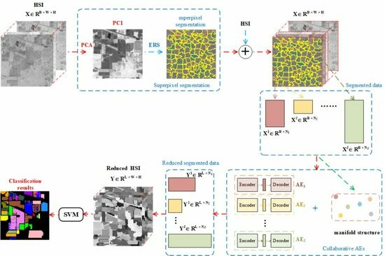
3. Collaborative Superpixelwise Auto-Encoder

In this section, we present the details of ColAE, a method designed for extracting spectral–spatial features for HSI. ColAE consists of two key steps: superpixel segmentation and collaborative AE learning, as depicted in Figure 3. During the superpixel segmentation step, the ERS-based superpixel method is employed to partition the HSI into homogeneous regions. This division creates compact and meaningful regions by grouping pixels with similar characteristics. In the collaborative learning step, LLE is first adopted to learn the underlying manifold structure among samples from different superpixels. This allows us to capture the global structure of the HSI. Next, AE models are applied to each superpixel independently. These models seek representations that minimize the local reconstruction error for samples within the same superpixel, while simultaneously minimizing the manifold reconstruction error for samples from different superpixels. In our proposed ColAE approach, the AE models exchange information among different superpixel regions, leveraging a collaborative learning approach. This enhances similar samples from different superpixels to be similar in the code space. In this way, ColAE can alleviate intra-class disparities. Figure 1c provides empirical evidence supporting this claim.

In this paper, HSI data are denoted by $\mathbf{X}\in {\mathbb{R}}^{B\times W\times H}$, where $B,W,H$ represent the number of spectral bands, width, and height, respectively. To process the 3D data $\mathbf{X}$, we flatten it into a 2D form, denoted as $\mathbf{X}\mathbf{2}=[{\mathbf{x}}_1,{\mathbf{x}}_2,\dots ,{\mathbf{x}}_N]\in {\mathbb{R}}^{B\times N}(N=W\times H)$. Each column ${\mathbf{x}}_i={[x_{i1},x_{i2},\dots ,x_{iB}]}^T$ represents a pixel in the HSI.

3.1. Superpixel Segmentation

Traditional spectral–spatial methods often use fix-sized spatial windows to incorporate spectral and spatial information. However, these methods do not fully explore the spatial information available in the image. Superpixel segmentation, on the other hand, offers a more effective way to divide the image into homogeneous regions based on appearance information, thereby considering spatial structures more effectively. This is why we have chosen to employ superpixel segmentation in our proposed work.

The Entropy Rate Segmentation (ERS) algorithm is capable of efficiently segmenting the grayscale (1 channel) or color (3 channels) images into superpixel regions. However, the HSI typically consists of hundreds of spectral bands. To address this, we first reduce the dimensionality of the HSI data to one channel using PCA before applying ERS.

PCA allows us to reduce an HSI, denoted as $\mathbf{X}$, to its 2D form $\mathbf{X}\mathbf{2}$. The covariance matrix of the data can be calculated using the formula $C=\frac{1}{N}\sum ({\mathbf{x}}_i-\mathit{\mu }){({\mathbf{x}}_i-\mathit{\mu })}^T$, where $\mathit{\mu }=\frac{1}{N}\sum {\mathbf{x}}_i$ is the mean vector of all samples. The eigenvectors ${\mathbf{v}}_1$ corresponding to the largest eigenvalue of C form the projection matrix $\mathbf{V}=\left[{\mathbf{v}}_1\right]$ for the grayscale image. Next, the 1-dimensional 2D data $\mathbf{Y}\mathbf{2}$ can is obtained by performing the transformation $\mathbf{Y}\mathbf{2}={\mathbf{V}}^T\mathbf{X}\mathbf{2}$. Finally, $\mathbf{Y}\mathbf{2}$ can be reshaped into a grayscale image, upon which ERS can be performed on the obtained superpixel segmentation.

3.2. Collaborative AEs

After performing superpixel segmentation on the HSI, the resulting 2D representation can be expressed as $\mathbf{X}\mathbf{2}=\{{\mathbf{X}}^1,{\mathbf{X}}^2,\dots ,{\mathbf{X}}^J\}$, where ${\mathbf{X}}^i=\{{\mathbf{x}}_1^i,{\mathbf{x}}_2^i,\dots ,{\mathbf{x}}_{N_i}^i\}$ represents the samples in the i-th superpixel, and $N_i$ indicates the number of samples in that particular superpixel.

To capture the underlying manifold structure of the data, samples from different superpixels are used. Then, an AE model is proposed to preserve this manifold structure among superpixels while simultaneously minimizing the reconstruction error within each superpixel. By jointly considering the manifold structure and the within-superpixel reconstruction, our proposed ColAE allows for the efficient extraction of spectral–spatial features while ensuring the preservation of important relationships between superpixels.

3.2.1. Learning the Manifold Structure among Superpixels

In order to preserve the relations among samples from different superpixels, it is crucial to define and obtain such relations. The manifold structure is commonly employed to model the underlying geometric structure of high-dimensional data, which aligns with our requirements. In our method, we adopt LLE, a classical and efficient manifold learning technique, to capture the manifold structure.

Samples within the same superpixel exhibit similarity; hence, the manifold structure is measured using only the mean vectors of each superpixel. The mean vector is calculated by

$${\mu }^i=\frac{1}{N_i}\sum _j{\mathbf{x}}_j^i.$$

(7)

With the mean vectors $\{{\mu }^1,{\mu }^2,\dots ,{\mu }^J\}$, the weighting matrix $\mathbf{W}$ can be obtained by minimizing the reconstruction error in Equation (2), where J is the number of superpixels. Denoting the representations in the i-th superpixel in code space as ${\mathbf{Y}}^i=\{{\mathbf{y}}_1^i,{\mathbf{y}}_2^i,\dots ,{\mathbf{y}}_{N_i}^i\}$, the manifold loss over current code is

$$\mathbf{L}\left(\mathbf{Y}\right)=\sum _i\Vert \sum _j\frac{1}{N_j}{\mathbf{y}}_j^i-\sum _k{w}_{ik}\sum _j\frac{1}{N_k}{\mathbf{y}}_j^k{\Vert }^2,$$

(8)

where ${\mathbf{M}}^Y=[\frac{1}{N_1}{\sum }_j{\mathbf{y}}_j^1,\frac{1}{N_2}{\sum }_j{\mathbf{y}}_j^2,\dots ,\frac{1}{N_J}{\sum }_j{\mathbf{y}}_j^J]$ represents the mean vectors in the code space. The lower the value of $\mathbf{L}\left(\mathbf{Y}\right)$, the better the preserving ability of the code.

It should be noted that the number of K, representing the number of nearest neighbors in the LLE algorithm, needs to be predefined when calculating the weighting matrix $\mathbf{W}$, and it is commonly chosen such that $K\ll J$.

3.2.2. AE Model with Manifold Constraints

Based on previous works [28,29,32], we adopt a similar approach and employ a single AE for each superpixel. In this way, multiple AEs are used to efficiently capture the local structure within a superpixel and low-dimensional representations of a given HSI can be obtained. The loss function for the i-th AE is defined as

$$\mathbf{R}\left({\mathsf{\Theta }}_i\right)=\sum _j\Vert {\mathbf{x}}_j^i-{\widehat{\mathbf{x}}}_j^i{\Vert }^2.$$

(9)

were ${\widehat{\mathbf{x}}}_j^i$ is the output of the i-th deep AE for the j-th sample ${\mathbf{x}}_j^i$ in the i-th superpixel. The parameters in this AE are denoted as ${\mathsf{\Theta }}_i=\{{\mathbf{W}}_i^{\left(1\right)},{\mathbf{b}}_i^{\left(1\right)},\dots ,{\mathbf{b}}_i^{\left(m\right)},{\mathbf{W}}_i^{\left(m\right)},\dots ,{\mathbf{W}}_i^{\left(2m\right)},{\mathbf{b}}_i^{\left(2m\right)}\}$, where m is the number of layers in encoder. The reconstruction error for all the samples can be expressed as

$$\mathbf{R}\left(\mathsf{\Theta }\right)=\sum _i\sum _j\Vert {\mathbf{x}}_j^i-{\widehat{\mathbf{x}}}_j^i{\Vert }^2,$$

(10)

where $\mathsf{\Theta }=\{{\mathsf{\Theta }}_1,{\mathsf{\Theta }}_2,\dots ,{\mathsf{\Theta }}_J\}$ represents the parameters for all AEs.

To preserve the relations among superpixels, the manifold loss in Equation (8) can be added to Equation (10). This results in the following loss function:

$$\mathbf{R}\left(\mathsf{\Theta }\right)=\sum _i\sum _j\Vert {\mathbf{x}}_j^i-{\widehat{\mathbf{x}}}_j^i{\Vert }^2+\eta \sum _i\Vert \sum _j\frac{1}{N_j}{\mathbf{y}}_j^i-\sum _k{w}_{ik}\sum _j\frac{1}{N_k}{\mathbf{y}}_j^k{\Vert }^2.$$

(11)

In Equation (11), the first term preserves the structure within each superpixel, while the second term maintains the structure between superpixels. The parameter $\eta$ balances the two terms. By incorporating two terms in Equation (11), the proposed ColAE ensures each AE can preserve the structure of data within its assigned superpixel, while exchange information between superpixel by considering the manifold structure. In this way, the AEs from each superpixel are collaboratively learned. It should be noted that, in Equation (11), the first term relates to all the parameters in $\mathsf{\Theta }$, while the second term only relates to the parameters in the encoder part.

To find the parameters that best fit the data, we first initial each AE using the Xavier method [38]. Then, we backpropagate the gradient of $\mathsf{\Theta }$ to each layer according to Equation (10). Since the number of samples in a superpixel is not large, we feed all the samples in each superpixel once to calculate the loss. After hundreds of iterations, the value of $\mathbf{R}\left(\mathsf{\Theta }\right)$ can converge to a small value.

3.3. Computational Analysis of ColAE

The procedure of the proposed ColAE is outlined in Algorithm 1. The time complexity of the proposed ColAE can be analyzed as follows. The superpixel segmentation step has a time complexity of $\mathcal{O}(\max (B^3,B^{2}N)+NlogN)$. The manifold structure modeling procedure has a time complexity of $\mathcal{O}\left(KJ\right)$, and the calculation of loss in Equation (10) has a time complexity of $\mathcal{O}\left(NB{d}_1\right)$, where $d_1$ is the dimensionality of the first hidden representation ${\mathbf{h}}^{\left(1\right)}$. The gradient descent method used to optimize the parameters $\mathsf{\Theta }$ has a time complexity of $\mathcal{O}\left(TNB{d}_1\right)$. In HSI, the number of bands B is typically much smaller than the number of samples N. Additionally, K and J are also much smaller than N. Therefore, the overall time complexity of ColAE is $\mathcal{O}\left(TNB{d}_1\right)$.

Algorithm 1 Procedures of ColAE.

Input: An HSI $\mathbf{X}\in {\mathbb{R}}^{B\times W\times H}$, the number of superpixels J, the number of nearest neighbors  K in LLE, the balancing weight $\eta$, the dimensionality L for the code, the number of  iteration T. Output: The output $\mathbf{Y}\in {\mathbb{R}}^{L\times W\times H}$. 1: Reshape $\mathbf{X}$ into 2D form, which is $\mathbf{X}\mathbf{2}\in {\mathbb{R}}^{B\times N}$. Use PCA to reduce the dimensionality  of $\mathbf{X}\mathbf{2}$ to 1, and reshape it into the image with three channels; 2: Apply ERS algorithm to segment the image into J non-overlapped regions; 3: Use Equation (7) to compute the mean vector ${\mu }_i$ for each superpixel. Then, calculate  the weights for each mean vector according to Equation (2); 4: Use Xavier initialization to initial the parameters in ${\mathsf{\Theta }}^{\left(0\right)}$; 5: for $t=0$ to T do 6:    Calculate the loss $R\left({\mathsf{\Theta }}^{\left(t\right)}\right)$ by Equation (11); 7:    Calculate the gradient of ${\mathbf{g}}^{\left(t\right)}$ using existing optimizer, and update the parameters by        ${\mathsf{\Theta }}^{(t+1)}={\mathsf{\Theta }}^{\left(t\right)}+\alpha {\mathbf{g}}^{\left(t\right)}$; 8: end for 9: Compute the code by ${\mathsf{\Theta }}^{\left(T\right)}$, then reshape the code into $\mathbf{Y}\in {\mathbb{R}}^{L\times W\times H}$. 10: return $\mathbf{Y}$.

4. Experimental Results

In this section, to validate the performance of the proposed ColAE, we carry out extensive experiments on several HSIs in comparison with state-of-the-art methods.

4.1. Data Sets

Three HSI data sets are used to evaluate the ColAE in our experiments, which are Indian Pines, the University of Pavia, and Salinas. The details of each data set are as follows.

(1)

Indian Pines. The Indian Pines data set was collected by the Airborne Visible/Infrared Imaging Spectrometer (AVIRIS) sensor over an agricultural area in Indiana, USA. It consists of $145\times 145$ pixels and 224 spectral bands, covering a wide range of wavelengths from 400 to 2500 nm. In this paper, 24 bands covering the region of water absorption are removed, and a total of 200 bands are used. The data set contains 16 different classes, including various crops, bare soil, and human-made structures. Approximately 10,249 samples with labels are from the ground-truth map.

(2)

University of Pavia. The University of Pavia data set was acquired by the Reflective Optics System Imaging Spectrometer (ROSIS) sensor over an agricultural area in Pavia, Italy. It consists of $610\times 340$ pixels and 115 spectral bands, covering wavelengths from 430 to 860 nm. A total of 12 noisy and water bands are removed, and a total of 103 bands are preserved. The data set contains nine different classes, including various crops, bare soil, and meadows. Approximately 42,776 samples with labels are from the ground-truth map.

(3)

Salinas. The Salinas data set was collected by the AVIRIS sensor over an agricultural area in Salinas Valley, California, USA. It consists of $512\times 217$ pixels and 224 spectral bands, covering wavelengths from 400 to 2500 nm. A total of 20 bands are removed for noisy and water bands, and 204 bands are used in our experiments. The data set contains 16 different classes, including various crops, bare soil, and human-made structures. A total of 53,129 labeled samples are used in our experiments.

Table 1. Number of samples in the Indian Pines, University of Pavia, and Salinas images.

	Indian Pines		University of Pavia		Salinas
	Class Name	Numbers	Class Name	Numbers	Class Name	Numbers
c1	Alfalfa	46	Asphalt	6631	Broccoli green weeds 1	2009
c2	Corn-notill	1428	Meadows	18,649	Broccoli green weeds 2	3726
c3	Corn-mintill	830	Gravel	2099	Fallow	1976
c4	Corn	237	Tress	3064	Fallow rough plow	1394
c5	Grass-pasture	483	Mental sheets	1345	Fallow smooth	2678
c6	Grass-tress	730	Bare soil	5029	Stubble	3959
c7	Grass-pasture-mowed	28	Bitumen	1330	Celery	2579
c8	Hay-windrowed	478	Bricks	3682	Grapes untrained	11271
c9	Oats	20	shadow	947	Soil vineyard develop	6203
c10	Soybean-nottill	972			Corn senesced green seed	3278
c11	Soybean-mintill	2455			Lettuce romaine 4wk	1068
c12	Soybean-clean	593			Lettuce romaine 5wk	1927
c13	Wheat	205			Lettuce romaine 6wk	916
c14	Woods	1265			Lettuce romaine 7wk	1070
c15	Buildings-grass-trees-dirves	386			Vineyard untrained	7268
c16	Stone-steel-towers	93			Vineyard vertical trellis	1807
	Total number	10,249	Total number	42,776	Total number	54,129

lists the number of samples per class for the three datasets. All these datasets are available (https://www.ehu.eus/ccwintco/index.php?title=Hyperspectral_Remote_Sensing_Scenes, accessed on 12 July 2021) from the Internet.

4.2. Experimental Setup

In the experiments, we evaluate the learned spectral–spatial feature via its classification performance. We use several well-known handcraft features, including PCA, LPP [39], KPCA [40], and their extensions to superpixel-based methods, SuperPCA [28], SuperLPP [41], SuperKPCA [31]. Deep learning-based features are compared, including AE [36], its superpixel extension version SuperAE, CAE [42], and ConstrastNet [43].

To test the proposed method, three metrics are used to evaluate the performance of different dimension reduction methods, which are overall accuracy (OA), average accuracy (AA), and kappa. The HSIs are used in their original form without any further preprocessing. We apply the DR algorithms on the HSI, then feed their outputs an SVM to determine the categories of the samples. The RBF kernel is used to boost the performance of the SVM for non-linear distributed situations, and the parameters of the RBF are determined by a grid search, as was performed in [28]. Our experiments are conducted on Windows 10 64-bit platform, with an Intel Core i5-12400F CPU (2.5 GHz), and 32 GB memory. The proposed approaches are implemented mainly using Python 3.6, Pytorch 1.8.0, Scikit-learn 1.2.1 (Sklearn), and Shogun (https://github.com/shogun-toolbox/shogun, accessed on 8 December 2020), which is a well-known machine learning toolbox that provides interfaces for Matlab, R, Python, and so on. With this feature, Shogun offers a convenient way to implement various machine learning algorithms easily.

To test the proposed method, the 10 random splits sets in [28] (https://github.com/junjun-jiang/SuperPCA/tree/master/datasets, accessed on 31 October 2020) are used for training and testing. For each class in the three data sets, $T=3,5,7,10,15,20$ samples are selected to train the SVM, and the rest of the samples are used as testing sets, where T denotes the number of training samples. For the classes that posses too few samples, such as Grass-pasture-mowed and Oats in Indian Pines, we select a maximum of half of the total samples in the them. The PCA, KPCA, and SVM are implemented by the Sklearn library. KPCA utilized the RBF kernel, and its best parameter is determined through a grid search based on the reconstruction error of the pre-image [44]. Moreover, LPP is implemented using the Shogun library, and the optimal number of nearest neighbors (K) and the $\tau$ for heat kernel are also determined using a grid search. The implementations for CAE and ConstrastNet are available (https://github.com/jjwwczy/ContrastNet-Unsupervised-Feature-Learning-by-Autoencoder-and-Prototypical-Contrastive-Learning, accessed on 8 March 2034) online. In our experiments, the architectures of AE and ColAE remain consistent, and are listed in

Table 2. The architecture of AE in the experiments. The shape is defined in Pytorch style, where −1 means batch size in the shape array.

Layer	Output Shape
	Indian Pines	University of Pavia	Salinas
input	[−1, 200]	[−1, 103]	[−1, 203]
Linear	[−1, 100]	[−1, 75]	[−1, 100]
Tanh	[−1, 100]	[−1, 75]	[−1, 100]
Linear	[−1, L]	[−1, L]	[−1, L]
Linear	[−1, 100]	[−1, 75]	[−1, 100]
Tanh	[−1, 100]	[−1, 75]	[−1, 100]
Linear	[−1, 200]	[−1, 103]	[−1, 203]

. For Equation (6), the tanh is used as the activation function when $m=1,4$, and the linear function is used when $m=2$ and $m=3$. Furthermore, Xavier initialization is employed to initial the parameters for both AE and ColAE. The ERS is also available (https://github.com/mingyuliutw/EntropyRateSuperpixel, accessed on 19 Auguest 2015) online. The SuperPCA, SuperNPE, SuperLPP, and SuperAE are applied based on the superpixel results obtained from ERS, according to their definitions as mentioned.

4.3. Comparisons with Other Algorithms

Table 3. Classification performance of the 13 methods on Indian Pines, University of Pavia, and Salinas images. T.N.s/C denotes the number of training samples from each class.

Data Set	T.N.s/C	Metric	Raw	PCA	LPP	KPCA	AE	Super PCA	Super LPP	Super KPCA	Contrast Net	CAE	SuperAE	ColAE
Indian Pines	3	OA(%)	40.89	40.89	45.01	40.81	40.37	54.55	58.28	48.28	55.20	54.50	67.78	68.81
		AA(%)	44.30	44.21	45.60	43.97	44.00	74.69	71.32	53.78	55.31	54.06	70.15	66.41
		kappa	0.3455	0.3455	0.3870	0.3451	0.3404	0.4837	0.5276	0.4415	0.4977	0.4942	0.6397	0.6518
	5	OA(%)	47.41	46.98	53.56	47.52	47.72	69.84	65.86	64.30	67.88	64.28	77.20	77.72
		AA(%)	48.60	48.38	52.23	48.43	48.65	80.91	76.43	61.22	60.73	60.81	77.49	74.79
		kappa	0.4156	0.4115	0.4818	0.4158	0.4190	0.6560	0.6149	0.6061	0.6364	0.5992	0.7429	0.7493
	7	OA(%)	51.38	50.84	58.47	51.46	50.65	77.01	75.00	77.62	73.36	70.20	81.34	82.03
		AA(%)	51.53	50.77	55.71	50.92	50.54	86.13	81.14	90.35	66.80	65.16	80.78	80.18
		kappa	0.4578	0.4516	0.5351	0.4566	0.4509	0.7378	0.7178	0.7364	0.6995	0.6651	0.7892	0.7969
	10	OA(%)	54.68	53.98	61.31	54.44	53.71	83.19	83.80	73.91	76.60	75.83	85.09	85.10
		AA(%)	54.00	53.46	58.90	53.66	52.98	85.31	80.25	87.48	70.11	69.57	82.84	81.96
		kappa	0.4943	0.4867	0.5669	0.4908	0.4840	0.8084	0.8092	0.7055	0.7369	0.7278	0.8311	0.8312
	15	OA(%)	58.83	57.60	64.56	58.29	56.86	87.81	86.23	87.82	80.02	80.96	87.69	88.02
		AA(%)	56.67	55.70	60.88	55.80	54.66	86.81	80.64	89.99	70.17	73.07	83.38	82.04
		kappa	0.5401	0.5267	0.6034	0.5328	0.5190	0.8611	0.8442	0.8620	0.7803	0.7852	0.8603	0.8640
	20	OA(%)	61.57	60.53	67.26	61.26	59.83	89.13	88.24	87.93	84.44	84.46	89.18	89.20
		AA(%)	57.39	56.48	60.89	56.98	56.35	85.17	83.61	89.66	75.13	74.89	81.28	80.98
		kappa	0.5694	0.5578	0.6326	0.5654	0.5503	0.8765	0.8726	0.8631	0.8237	0.8241	0.8771	0.8773
University of Pavia	3	OA(%)	60.50	60.55	54.40	-	61.03	78.48	67.41	81.83	79.71	70.52	83.66	84.04
		AA(%)	64.73	64.62	56.80	-	65.25	73.94	72.72	73.99	81.67	74.61	83.54	84.01
		kappa	0.5154	0.5157	0.4341	-	0.5203	0.7222	0.5736	0.7615	0.7333	0.6239	0.7911	0.7957
	5	OA(%)	65.77	65.73	58.22	-	65.03	82.02	71.49	85.06	83.49	78.89	87.21	87.40
		AA(%)	68.53	68.49	59.97	-	68.56	78.94	75.25	80.49	85.11	81.10	86.40	86.70
		kappa	0.5731	0.5727	0.4788	-	0.5671	0.7675	0.6297	0.8061	0.7813	0.7300	0.8366	0.8390
	7	OA(%)	70.36	70.34	60.02	-	69.01	84.40	74.98	86.92	87.81	84.75	88.83	89.43
		AA(%)	72.03	71.92	61.92	-	70.70	82.89	79.18	83.32	86.66	84.79	87.24	87.65
		kappa	0.6253	0.6247	0.5016	-	0.6107	0.7988	0.6714	0.8305	0.8393	0.8033	0.8564	0.8638
	10	OA(%)	72.66	72.48	63.43	-	71.46	89.01	80.24	91.09	91.95	88.83	92.53	92.74
		AA(%)	74.12	73.95	64.54	-	72.85	87.22	83.33	89.87	90.37	87.97	90.94	91.10
		kappa	0.6553	0.6532	0.5450	-	0.6414	0.8577	0.7387	0.8836	0.8939	0.8545	0.9031	0.9057
	15	OA(%)	77.90	78.26	65.48	-	76.26	91.86	81.26	92.30	94.38	92.03	94.76	94.93
		AA(%)	77.03	77.13	66.57	-	75.32	89.56	83.74	91.29	92.70	90.55	93.10	93.29
		kappa	0.7169	0.7210	0.5734	-	0.6975	0.8938	0.7549	0.8982	0.9257	0.8957	0.9314	0.9337
	20	OA(%)	80.57	80.66	70.13	-	79.35	92.60	82.48	91.37	95.01	94.08	95.16	95.39
		AA(%)	78.84	78.84	69.32	-	77.40	90.79	85.38	89.52	93.34	92.49	93.29	93.61
		kappa	0.7497	0.7512	0.6254	-	0.7346	0.9034	0.7714	0.8865	0.9343	0.9222	0.9365	0.9396
Salinas	3	OA(%)	79.13	79.15	78.22	-	80.86	70.21	75.30	76.84	80.21	80.84	88.14	89.46
		AA(%)	83.48	83.48	83.38	-	86.34	73.75	79.16	89.20	81.93	84.38	90.91	92.43
		kappa	0.7687	0.7688	0.7598	-	0.7877	0.6729	0.7217	0.7435	0.7808	0.7874	0.8681	0.8828
	5	OA(%)	81.13	81.09	82.21	-	82.48	80.67	80.97	80.46	84.98	87.12	90.97	91.97
		AA(%)	85.86	85.88	87.55	-	87.96	84.59	87.58	78.96	86.78	89.04	94.29	94.77
		kappa	0.7906	0.7901	0.8035	-	0.8056	0.7859	0.7871	0.7835	0.8330	0.8570	0.8997	0.9108
	7	OA(%)	83.68	83.66	83.58	-	84.63	88.20	90.21	87.46	87.18	89.92	93.25	94.01
		AA(%)	87.79	87.74	88.09	-	89.47	90.75	93.69	90.28	88.62	91.18	95.94	96.21
		kappa	0.8188	0.8186	0.8176	-	0.8293	0.8692	0.8906	0.8602	0.8576	0.8883	0.9251	0.9334
	10	OA(%)	85.45	85.27	84.71	-	85.94	91.38	90.59	89.58	88.71	91.98	94.53	94.83
		AA(%)	89.15	89.09	89.30	-	90.34	94.45	93.99	93.03	90.26	92.91	96.51	96.61
		kappa	0.8382	0.8362	0.8305	-	0.8437	0.9036	0.8948	0.8892	0.8747	0.9109	0.9392	0.9426
	15	OA(%)	86.89	86.77	86.04	-	87.28	95.26	92.69	92.36	91.59	94.10	96.06	96.14
		AA(%)	90.63	90.55	90.68	-	91.45	96.10	94.32	94.66	92.48	94.69	97.18	97.27
		kappa	0.8543	0.8530	0.8450	-	0.8587	0.9471	0.9174	0.9146	0.9066	0.9345	0.9562	0.9571
	20	OA(%)	88.14	88.16	88.39	-	88.16	97.06	94.62	94.25	92.84	95.52	97.06	97.20
		AA(%)	91.44	91.48	91.80	-	92.09	96.89	93.43	94.38	93.70	95.91	97.55	97.63
		kappa	0.8680	0.8682	0.8809	-	0.8666	0.9633	0.9403	0.9359	0.9204	0.9503	0.9673	0.9687

presents the performances of features acquired by 13 methods on the three data sets with diverse training samples when $L=30$, where L is the dimensionality of the low-dimensional representation. The best classification results in each setting are highlighted in bold. It is worth noting that KPCA consumes too much memory, making it impossible to execute in the University of Pavia and Salinas data sets. From the results in Table 3, several observations can be concluded as follows.

1. In nearly all tested scenarios, the efficacy of our proposed ColAE method surpasses that of the other approaches, highlighting its superior performance. It is important to note that, in the Indian Pines data set, SuperPCA exhibits better average accuracy (AA) results than ColAE. However, when evaluated based on overall accuracy (OA) and kappa, ColAE outperforms SuperPCA. Upon further analysis of the classification outcomes, we present the observation that ColAE consistently exhibits superior performance on categories with larger sample sizes, while its performance diminishes on categories with fewer samples, as illustrated in

Table 4. Classification results for each class in Indian Pines when 15 training samples are used.

	Raw	PCA	LPP	KPCA	AE	Super PCA	Super LPP	Super KPCA	Contrast Net	CAE	SuperAE	ColAE
c1	34.70	35.91	40.57	31.72	31.17	100.00	100.00	100.00	53.45	64.65	100.00	98.81
c2	47.50	45.38	54.40	46.80	44.93	78.82	75.48	58.02	78.22	72.38	78.10	78.89
c3	36.87	34.91	42.88	36.10	38.18	91.56	99.53	96.23	68.63	75.18	87.41	83.61
c4	32.52	30.66	40.47	31.64	28.79	82.44	69.10	86.56	48.66	58.29	69.31	65.46
c5	66.76	65.47	67.28	66.76	63.60	98.55	97.01	99.76	91.74	85.49	97.31	96.12
c6	89.97	89.40	88.21	89.38	88.07	99.80	99.43	100.00	93.11	90.27	99.76	99.89
c7	22.17	20.98	23.44	21.52	20.77	50.80	39.39	34.21	26.00	45.89	59.74	51.95
c8	98.39	98.32	96.91	98.33	98.41	98.57	98.72	100.00	97.68	94.95	99.98	100.00
c9	8.25	7.54	14.74	7.51	5.97	45.59	10.20	100.00	22.73	16.52	35.19	21.74
c10	50.52	48.54	59.45	47.62	48.85	90.91	95.05	95.83	79.52	80.00	83.84	85.78
c11	70.36	72.25	80.06	70.02	73.29	87.94	95.61	98.71	87.54	89.22	93.54	94.20
c12	43.09	39.19	54.22	41.98	33.23	85.07	87.76	88.77	68.76	72.79	70.46	76.54
c13	82.80	81.65	83.30	80.81	82.05	100.00	100.00	100.00	81.66	84.36	99.79	100.00
c14	92.84	92.56	93.84	92.36	92.28	92.49	71.27	98.42	93.62	94.81	98.56	98.56
c15	36.92	35.50	42.04	37.32	33.08	97.51	91.96	99.46	66.97	71.13	92.72	92.18
c16	93.10	92.98	92.32	93.00	91.87	88.96	59.69	83.87	64.46	73.20	68.31	68.88
AA	56.67	55.70	60.88	55.80	54.66	86.81	80.64	89.99	70.17	73.07	83.38	82.04
OA	58.83	57.60	64.56	58.29	56.86	87.81	86.23	87.82	80.20	80.96	87.69	88.02

,

Table 5. Classification results for each class in the University of Pavia when 20 training samples are used.

	Raw	PCA	LPP	AE	Super PCA	Super LPP	Super KPCA	Contrast Net	CAE	SuperAE	ColAE
c1	93.94	93.93	92.52	93.55	92.42	93.51	89.13	96.12	95.21	97.53	97.68
c2	91.48	90.93	88.97	91.67	98.33	86.62	97.58	99.08	98.87	98.88	98.85
c3	59.62	59.37	46.08	55.17	94.71	89.98	98.53	93.16	90.39	93.60	93.63
c4	70.22	69.52	65.85	69.50	69.54	80.28	76.85	84.02	81.28	77.95	78.38
c5	95.80	96.01	74.25	96.43	98.00	96.95	96.61	99.98	98.94	99.86	99.86
c6	62.08	63.36	44.53	62.07	99.02	54.54	98.56	96.53	95.06	98.00	99.16
c7	57.60	57.69	45.10	51.67	78.53	75.68	77.10	89.19	90.38	80.96	82.28
c8	57.60	57.69	45.10	51.67	78.53	75.68	71.89	83.61	84.28	80.96	82.28
c9	99.94	99.95	99.99	99.95	99.81	99.46	99.43	98.30	97.98	99.84	99.88
AA	78.84	78.84	69.32	77.40	90.79	85.38	89.52	93.34	92.49	93.30	93.61
OA	80.57	80.66	70.13	79.35	92.60	82.48	91.37	95.02	94.08	95.16	95.39

and

Table 6. Classification results for each class in Salinas when 20 training samples are used.

	Raw	PCA	LPP	AE	Super PCA	Super LPP	Super KPCA	Contrast Net	CAE	SuperAE	ColAE
c1	97.70	97.70	99.38	98.74	99.97	100.00	100.00	97.07	98.84	100.00	100.00
c2	98.46	98.43	98.37	99.07	99.85	99.17	100.00	96.31	99.00	99.88	99.88
c3	91.23	91.16	89.20	91.73	98.52	98.23	96.05	95.95	96.08	99.99	99.79
c4	96.92	96.93	98.76	97.25	96.70	95.86	97.23	93.71	82.88	96.57	96.57
c5	96.71	96.69	95.07	96.58	95.67	77.29	95.76	91.82	98.68	98.29	98.14
c6	99.78	99.78	99.72	99.95	99.18	100.00	99.82	99.68	99.72	100.00	100.00
c7	98.41	98.35	98.66	99.03	99.70	99.68	99.83	94.04	99.39	99.76	99.80
c8	78.45	77.98	78.25	78.54	98.33	99.92	91.29	90.08	95.41	98.04	97.18
c9	98.89	98.84	99.24	99.23	98.05	98.04	90.32	98.61	99.67	99.13	99.12
c10	84.89	85.56	81.05	86.07	94.58	88.31	88.43	95.29	95.48	91.68	91.85
c11	78.10	77.99	75.48	80.91	88.41	62.57	89.76	77.67	89.15	98.79	98.68
c12	95.79	95.82	96.70	96.69	94.39	97.79	83.71	96.75	97.50	98.79	98.82
c13	94.76	94.65	98.99	96.43	98.21	99.55	96.10	93.98	98.56	98.63	98.12
c14	86.24	86.06	92.66	89.05	90.93	88.71	85.20	97.68	97.78	91.63	92.63
c15	68.46	69.54	69.06	66.18	98.57	90.82	99.87	84.75	87.41	90.34	92.32
c16	98.22	98.28	98.16	98.01	99.15	98.99	96.77	95.85	98.99	99.29	99.25
AA	91.44	91.48	91.80	92.09	96.89	93.43	94.38	93.70	95.91	97.55	97.63
OA	88.14	88.16	88.39	88.16	97.06	94.62	94.25	92.84	95.52	97.06	97.20

. This phenomenon is mainly because the proposed ColAE utilizes LLE to model the manifold structure between superpixels. LLE employs the concept of K-nearest neighbors, where K is often set to a value much smaller than the total number of samples, to capture the local structure of the data. However, categories with only a few samples tend to be confined within a limited number of superpixels. Consequently, when modeling the manifold structure, LLE might incorrectly associate these small categories with others, leading to a lower classification accuracy for categories with a small sample size. In cases where a category has sufficient samples, these samples are always located in a set of superpixels, typically surpassing the value of K. Consequently, the inherent structure can be effectively modeled and preserved by ColAE. In this way, the disparity problem can be well solved, leading to a higher classification.

2. ColAE consistently outperforms SuperAE, which proves that the proposed regularization term in Equation (11) can efficiently solve the class disparity problem caused by the superpixel-based method. To validate our findings, we randomly select one split from each data set and map the classification results onto the corresponding images, as shown in Figure 4, Figure 5 and Figure 6. A comparison between Figure 4n,o reveals that ColAE improves the accuracy by mainly relying on correctly classifying the large regions of Soybean-min-till, indicated in pink. Remarkably, based on the superpixel segmentation, it is observed that SuperAE misclassifies samples belonging to the Soybean-min-till class within a superpixel into Soybean-not-till (indicated in blue). In contrast, ColAE successfully minimizes the misclassification rate within the same region, highlighting the efficiency of the proposed graph-regularization term in Equation (11).

3. The performances of features obtained solely from the spectral domain are significantly inferior to those obtained from the spectral–spatial domain, substantiating the importance of incorporating information from the spatial domain for classification purposes. Both SuperAE and ColAE outperform ContrastNet and CAE, despite the fact that the architecture of the network is more complex in ContrastNet and CAE compared to SuperAE and ColAE. This outcome validates the superiority of superpixel-based methods. Additionally, the superpixel-based method consumes much fewer computational resources. Because the unsupervised method process all the data by DR models, then splits the data into training and testing sets, KPCA consumes 207,400 × 207,400 × 4 ≈ 160 GB memory for the University of Pavia and 111,104 × 111,104 × 4 ≈ 46 GB memory for Salinas, with a single-precious point floating point when constructing the kernel matrix. SuperKPCA consumes significantly less memory compared to traditional KPCA, further emphasizing the flexibility of superpixel-based approaches.

4. SuperPCA demonstrates surprisingly strong performance across all settings, which indicates the underlying data structure within a superpixel is relatively simple. That finding justifies our use of an AE with only two layers in both the encoder and decoder. The superior performance of both SuperAE and ColAE, compared to SuperPCA, further emphasizes the enhanced generalization ability. Additionally, it is worth noting that SuperKPCA and SuperLPP do not consistently outperform SuperPCA. We attribute this to the fact that the grid-search strategy employed in parameter tuning requires the inclusion of the best parameters within the search space. However, as the data distribution varies from one superpixel to another, it is challenging to accurately tune the parameters of SuperKPCA and SuperLPP to achieve optimal performance.

5. The performances of PCA on the three data sets are observed to be comparable to that of the raw feature. The proportion of retained principal components in PCA is 99.25% for Indian Pines, 99.96% for the University of Pavia, and 99.99% for Salinas. These results indicate that PCA can remove the components without valuable information, resulting in little accuracy loss. LPP and KPCA outperform PCA due to the inherent complexity of the underlying data structure in the HSIs. LPP and KPCA can preserve the nonlinear structure of the data, thus yielding improved classification performance. It is interesting that AE performs slightly inferior to raw and PCA. This can be attributed to the limited capacity of a two-layer encoder with only a single nonlinear function to capture the intricate data structure. Utilizing neural networks with more complex architectures can improve the accuracy of the AE. It is important to highlight that we maintained uniform architecture across AE, SuperAE, and ColAE intentionally, aiming to discern the influence of the superpixel-based technique and the introduced regularization term specified in Equation (11). Consequently, we do not design a distinct structure for AE within our experimental setup.

It is important to highlight that we maintained uniform architecture across AE, SuperAE, and ColAE intentionally, aiming to discern the influence of the superpixel-based technique and the introduced regularization term specified in Equation (11). Consequently, we refrained from designing a distinct structure for the AE within our experimental setup.

4.4. Parameter Analyses

In the proposed ColAE, several parameters need to be predefined: the number of superpixels J, the number of nearest neighbors K in the LLE, the balancing weight $\eta$, and the dimensionality L for the code. Actually, J is intertwined with K, where K is usually far smaller than J.To strengthen the relationships between the parameters, a ratio (R) can be introduced, which establishes a connection between K and J as $K=\lfloor J\times R\rfloor$, where $\lfloor ·\rfloor$ denotes the round operator, ensuring that K is an integer value. This approach ensures that the choice of K is directly proportional to the number of superpixels J by a factor determined by R. $\eta$ is also influenced by J and K, since it is impacted by the number of samples within a superpixel, which in turn affects the loss values of the terms in Equation (11). Therefore, our analysis starts with a discussion of L, then examines K, J, and $\eta$ by considering their interconnected relationship.

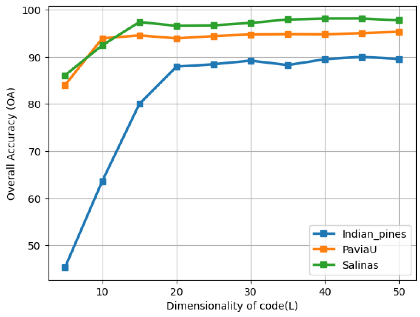
4.4.1. The Effect of the Dimensionality of the Code

In our experiments, we set $K=100$ for Indian Pines and Salinas, and $K=20$ for the University of Pavia. Additionally, we use a fixed ratio $R=0.2$ to determine the value of K. Furthermore, we choose $\eta =0.75$. To investigate the effect of the dimensionality of the code L, we vary L from 5 to 50 with an interval of 5, and examine the resulting overall classification accuracies with $T=20$ for SVM. The comprehensive experimentation yielded significant insights. For instance, in the case of dimensionality L, the highest Overall Accuracy (OA) of 89.98% was achieved when $L=45$ for the Indian Pines data set. Conversely, the lowest OA of 45.34% was observed at $L=5$. Similar trends were discerned for the University of Pavia dataset, where OA ranged from 84.01% to 95.30%, and for the Salinas dataset, where OA varied between 86.09% and 98.14%. To provide a more insightful depiction of these findings, these results are illustrated in Figure 7.

It is evident from the figure that when $L=5$, the OAs are low across all three data sets, which aligns with common sense. A small number of features restricts the ability to carry sufficient discriminative information for effective classification. However, as L increases, the OAs steadily improve. A relatively large value of L is reached where the growth of OAs becomes slow, indicating that the available discriminative information is already well utilized. A larger L will increase the complexity and computational requirements of the classifier without yielding significant performance gains. Based on the observations, we choose $L=30$ for all the subsequent experiments.

4.4.2. The Effects of the Number of Superpixels, Number of Nearest Neighbors, and Balance Weight

We set dimensionality of the code L to be 30, and varied the balance weight $\eta$ within the range of $[0.5,0.75,1,1.25]$, as well as the number of superpixels J from the set $[20,50,70,100,$$120,150]$. Additionally, we examined the ratio R between J and K, considering values from the set $[0.1,0.2,0.3,0.4]$, to evaluate the performance of the ColAE on three data sets. Across the above configurations of these parameters, OA spanned from 85.39% to 89.37% for Indian Pines, from 88.25% to 95.06% for University of Pavia, and from 94.01% to 97.38% for Salinas. The classification accuracies obtained from these experiments are also presented in Figure 8.

A notable observation is that the number of superpixels J emerges as the primary factor influencing the performance of ColAE. On the Indian Pines, the classification accuracy of ColAE initially increases and then decreases with the increment of J. This may be attributed to the rich texture information presented in this data set. Too few superpixels can cause different class samples to be merged together, while an excessive number of superpixels may result in too few samples in a superpixel, consequently limiting the learning capabilities of AE within the ColAE framework. Conversely, for the University of Pavia and Salinas data sets, classification accuracy declines if J is set too large. This trend could be attributed to the samples being clustered together in these data sets, where a small number of superpixels is sufficient for effective segmentation. Furthermore, it is worth noting that ColAE is robust with the number of nearest neighbors K and balance weight $\eta$, making it adaptable for application to other data sets.

4.4.3. Execution Time

In this work, all the experiments are conducted on a desktop. The implemented codes use the CPU for execution. The running times of nine DR methods on the three data sets are presented in

Table 7. Training time (in seconds) of nine DR methods on three HSI data sets.

	PCA	LPP	KPCA	AE	SuperPCA	SuperLPP	SuperKPCA	SuperAE	ColAE
Indian Pines	0.09	85.12	628.87	53.23	1.03	90.64	524.66	58.34	58.45
University of Pavia	0.91	104.21	-	214.12	1.22	277.22	1245.12	158.58	160.10
Salinas	0.73	102.12	-	198.72	1.47	232.98	1862.23	132.43	134.22

. It is worth noting that, compared with the training time, projecting the samples onto low-dimensional space demands minimal computational time once the model has been already trained. So we only list the training time in this section. It is important to note that the implementations of CAE and ContrastNet use the GPU to accelerate the training process. However, to ensure fairness in comparing the computational times across different methods, the running times of CAE and ConstrastNet are not included. The number of samples to be processed is 145 × 145 = 21,025 for Indian Pines, 610 × 340 = 207,400 for the University of Pavia, and 512 × 217 = 111,104 for the Salinas.

As indicated in Table 7, PCA exhibits the lowest computational time due to its parameter-free nature. On the other hand, KPCA and SuperKPCA consume the most time, since the parameter $\tau$ needs to be tuned and both methods construct a dense kernel matrix of size $N\times N$. The grid search strategy employed for parameter tuning further increases their computational burden. In contrast, LPP and SuperLPP also use the grid search for parameter tuning, but they only construct a sparse matrix with $K\times K$ entries, significantly reducing the computational burden. The proposed ColAE requires a similar computational time to SuperAE, although ColAE involves an additional step of constructing a manifold graph matrix. However, the size of the graph matrix is relatively small, being $J\times J$. It should be noted that, while all samples within a superpixel are fed into the optimizer in SuperAE and ColAE, the batch size for AE is set to 256. Hence, the computational time of AE is longer compared to SuperAE and ColAE. Furthermore, it is worth mentioning that the computational time of AE, SuperAE, and ColAE can be greatly reduced when GPU is employed for parallel computation.

5. Conclusions

In this paper, we have discovered that existing superpixel-based DR methods may disrupt the intra-structure of the data. To solve this problem, an unsupervised spectral–spatial DR method called ColAE is proposed. In ColAE, the HSI is first segmented into superpixels, then an LLE graph is constructed to model the similarities between the mean vectors from each superpixel. A set of AEs is applied to the samples within each superpixel, with the LLE graph employed to reduce the intra-disparity of the representations in code space. Experimental results on three HSI data sets can validate the effectiveness of the proposed ColAE in addressing the challenges of superpixel-based DR methods.

It should be noted that the ColAE can be extended to a multiscale superpixel version, which is expected to yield higher classification accuracy. Additionally, exploring the utilization of other manifold learning-based graphs can to model the relationship between superpixels will be a focal point for future research efforts.

References

1. Sun, W.; Du, Q. Hyperspectral band selection: A review. IEEE Geosci. Remote Sens. Mag. 2019, 7, 118–139. [Google Scholar] [CrossRef]
2. Rasti, B.; Hong, D.; Hang, R.; Ghamisi, P.; Kang, X.; Chanussot, J.; Benediktsson, J.A. Feature extraction for hyperspectral imagery: The evolution from shallow to deep: Overview and toolbox. IEEE Geosci. Remote Sens. Mag. 2020, 8, 60–88. [Google Scholar] [CrossRef]
3. Jia, X.; Kuo, B.C.; Crawford, M.M. Feature mining for hyperspectral image classification. Proc. IEEE 2013, 101, 676–697. [Google Scholar] [CrossRef]
4. Schwaller, M.R. A geobotanical investigation based on linear discriminant and profile analyses of airborne thematic mapper simulator data. Remote Sens. Environ. 1987, 23, 23–34. [Google Scholar] [CrossRef]
5. Bandos, T.V.; Bruzzone, L.; Camps-Valls, G. Classification of hyperspectral images with regularized linear discriminant analysis. IEEE Trans. Geosci. Remote Sens. 2009, 47, 862–873. [Google Scholar] [CrossRef]
6. Du, Q. Modified Fisher’s linear discriminant analysis for hyperspectral imagery. IEEE Geosci. Remote Sens. Lett. 2007, 4, 503–507. [Google Scholar] [CrossRef]
7. Fabiyi, S.D.; Murray, P.; Zabalza, J.; Ren, J. Folded LDA: Extending the linear discriminant analysis algorithm for feature extraction and data reduction in hyperspectral remote sensing. IEEE J. Sel. Top. Appl. Earth Obs. Remote Sens. 2021, 14, 12312–12331. [Google Scholar] [CrossRef]
8. Li, W.; Prasad, S.; Fowler, J.E.; Bruce, L.M. Locality-preserving discriminant analysis in kernel-induced feature spaces for hyperspectral image classification. IEEE Geosci. Remote Sens. Lett. 2011, 8, 894–898. [Google Scholar] [CrossRef]
9. Chen, M.; Wang, Q.; Li, X. Discriminant analysis with graph learning for hyperspectral image classification. Remote Sens. 2018, 10, 836. [Google Scholar] [CrossRef]
10. Luo, F.; Zhang, L.; Du, B.; Zhang, L. Dimensionality reduction with enhanced hybrid-graph discriminant learning for hyperspectral image classification. IEEE Trans. Geosci. Remote Sens. 2020, 58, 5336–5353. [Google Scholar] [CrossRef]
11. Ly, N.H.; Du, Q.; Fowler, J.E. Sparse graph-based discriminant analysis for hyperspectral imagery. IEEE Trans. Geosci. Remote Sens. 2013, 52, 3872–3884. [Google Scholar]
12. Luo, F.; Zhang, L.; Zhou, X.; Guo, T.; Cheng, Y.; Yin, T. Sparse-adaptive hypergraph discriminant analysis for hyperspectral image classification. IEEE Geosci. Remote Sens. Lett. 2019, 17, 1082–1086. [Google Scholar] [CrossRef]
13. Lim, S.; Sohn, K.H.; Lee, C. Principal component analysis for compression of hyperspectral images. In Proceedings of the IGARSS 2001, Sydney, NSW, Australia, 9–13 July 2001; Volume 1, pp. 97–99. [Google Scholar]
14. Rodarmel, C.; Shan, J. Principal component analysis for hyperspectral image classification. Surv. Land Inf. Sci. 2002, 62, 115–122. [Google Scholar]
15. Machidon, A.L.; Del Frate, F.; Picchiani, M.; Machidon, O.M.; Ogrutan, P.L. Geometrical approximated principal component analysis for hyperspectral image analysis. Remote Sens. 2020, 12, 1698. [Google Scholar] [CrossRef]
16. Ma, L.; Crawford, M.M.; Tian, J. Local manifold learning-based k-nearest-neighbor for hyperspectral image classification. IEEE Trans. Geosci. Remote Sens. 2010, 48, 4099–4109. [Google Scholar] [CrossRef]
17. Hong, D.; Yokoya, N.; Zhu, X.X. Learning a robust local manifold representation for hyperspectral dimensionality reduction. IEEE J. Sel. Top. Appl. Earth Obs. Remote Sens. 2017, 10, 2960–2975. [Google Scholar] [CrossRef]
18. Yu, W.; Zhang, M.; Shen, Y. Learning a local manifold representation based on improved neighborhood rough set and LLE for hyperspectral dimensionality reduction. Signal Process. 2019, 164, 20–29. [Google Scholar] [CrossRef]
19. Camps-Valls, G.; Marsheva, T.V.B.; Zhou, D. Semi-supervised graph-based hyperspectral image classification. IEEE Trans. Geosci. Remote Sens. 2007, 45, 3044–3054. [Google Scholar] [CrossRef]
20. Liao, W.; Pizurica, A.; Scheunders, P.; Philips, W.; Pi, Y. Semisupervised local discriminant analysis for feature extraction in hyperspectral images. IEEE Trans. Geosci. Remote Sens. 2012, 51, 184–198. [Google Scholar] [CrossRef]
21. Shao, Z.; Zhang, L. Sparse dimensionality reduction of hyperspectral image based on semi-supervised local Fisher discriminant analysis. Int. J. Appl. Earth Obs. Geoinf. 2014, 31, 122–129. [Google Scholar] [CrossRef]
22. Chen, Y.; Lin, Z.; Zhao, X.; Wang, G.; Gu, Y. Deep learning-based classification of hyperspectral data. IEEE J. Sel. Top. Appl. Earth Obs. Remote Sens. 2014, 7, 2094–2107. [Google Scholar] [CrossRef]
23. Zhou, P.; Han, J.; Cheng, G.; Zhang, B. Learning compact and discriminative stacked autoencoder for hyperspectral image classification. IEEE Trans. Geosci. Remote Sens. 2019, 57, 4823–4833. [Google Scholar] [CrossRef]
24. Chen, Y.; Huang, L.; Zhu, L.; Yokoya, N.; Jia, X. Fine-grained classification of hyperspectral imagery based on deep learning. Remote Sens. 2019, 11, 2690. [Google Scholar] [CrossRef]
25. He, N.; Paoletti, M.E.; Haut, J.M.; Fang, L.; Li, S.; Plaza, A.; Plaza, J. Feature extraction with multiscale covariance maps for hyperspectral image classification. IEEE Trans. Geosci. Remote Sens. 2018, 57, 755–769. [Google Scholar] [CrossRef]
26. Fang, L.; He, N.; Li, S.; Plaza, A.J.; Plaza, J. A new spatial–spectral feature extraction method for hyperspectral images using local covariance matrix representation. IEEE Trans. Geosci. Remote Sens. 2018, 56, 3534–3546. [Google Scholar] [CrossRef]
27. Li, N.; Zhou, D.; Shi, J.; Wu, T.; Gong, M. Spectral-locational-spatial manifold learning for hyperspectral images dimensionality reduction. Remote Sens. 2021, 13, 2752. [Google Scholar] [CrossRef]
28. Jiang, J.; Ma, J.; Chen, C.; Wang, Z.; Cai, Z.; Wang, L. SuperPCA: A superpixelwise PCA approach for unsupervised feature extraction of hyperspectral imagery. IEEE Trans. Geosci. Remote Sens. 2018, 56, 4581–4593. [Google Scholar] [CrossRef]
29. Zhang, X.; Jiang, X.; Jiang, J.; Zhang, Y.; Liu, X.; Cai, Z. Spectral–spatial and superpixelwise PCA for unsupervised feature extraction of hyperspectral imagery. IEEE Trans. Geosci. Remote Sens. 2022, 60, 1–10. [Google Scholar] [CrossRef]
30. Zhang, A.; Pan, Z.; Fu, H.; Sun, G.; Rong, J.; Ren, J.; Jia, X.; Yao, Y. Superpixel nonlocal weighting joint sparse representation for hyperspectral image classification. Remote Sens. 2022, 14, 2125. [Google Scholar] [CrossRef]
31. Zhang, L.; Su, H.; Shen, J. Hyperspectral dimensionality reduction based on multiscale superpixelwise kernel principal component analysis. Remote Sens. 2019, 11, 1219. [Google Scholar] [CrossRef]
32. Liang, M.; Jiao, L.; Meng, Z. A superpixel-based relational auto-encoder for feature extraction of hyperspectral images. Remote Sens. 2019, 11, 2454. [Google Scholar] [CrossRef]
33. Van der Maaten, L.; Hinton, G. Visualizing data using t-SNE. J. Mach. Learn. Res. 2008, 9, 2579–2605. [Google Scholar]
34. Liu, M.Y.; Tuzel, O.; Ramalingam, S.; Chellappa, R. Entropy rate superpixel segmentation. In Proceedings of the CVPR 2011, Colorado Springs, CO, USA, 20–25 June 2011; pp. 2097–2104. [Google Scholar]
35. Roweis, S.T.; Saul, L.K. Nonlinear dimensionality reduction by locally linear embedding. Science 2000, 290, 2323–2326. [Google Scholar] [CrossRef]
36. Hinton, G.E.; Salakhutdinov, R.R. Reducing the dimensionality of data with neural networks. Science 2006, 313, 504–507. [Google Scholar] [CrossRef]
37. He, K.; Zhang, X.; Ren, S.; Sun, J. Delving deep into rectifiers: Surpassing human-level performance on imagenet classification. In Proceedings of the ICCV 2015, Santiago, Chile, 7–13 December 2015; pp. 1026–1034. [Google Scholar]
38. Glorot, X.; Bengio, Y. Understanding the difficulty of training deep feedforward neural networks. In Proceedings of the Thirteenth International Conference on Artificial Intelligence and Statistics, Sardinia, Italy, 13–15 May 2010; pp. 249–256. [Google Scholar]
39. He, X.; Niyogi, P. Locality preserving projections. Adv. Neural Inf. Process. Syst. 2003, 16, 186–197. [Google Scholar]
40. Schölkopf, B.; Smola, A.; Müller, K.R. Kernel principal component analysis. In International Conference on Artificial Neural Networks; Springer: Berlin, Germany, 1997; pp. 583–588. [Google Scholar]
41. He, L.; Chen, X.; Li, J.; Xie, X. Multiscale superpixelwise locality preserving projection for hyperspectral image classification. Appl. Sci. 2019, 9, 2161. [Google Scholar] [CrossRef]
42. Mei, S.; Ji, J.; Geng, Y.; Zhang, Z.; Li, X.; Du, Q. Unsupervised spatial-spectral feature learning by 3D convolutional autoencoder for hyperspectral classification. IEEE Trans. Geosci. Remote Sens. 2019, 57, 6808–6820. [Google Scholar] [CrossRef]
43. Cao, Z.; Li, X.; Feng, Y.; Chen, S.; Xia, C.; Zhao, L. ContrastNet: Unsupervised feature learning by autoencoder and prototypical contrastive learning for hyperspectral imagery classification. Neurocomputing 2021, 460, 71–83. [Google Scholar] [CrossRef]
44. Bakır, G.H.; Weston, J.; Schölkopf, B. Learning to find pre-images. Adv. Neural Inf. Process. Syst. 2004, 16, 449–456. [Google Scholar]
Figure 1. Visualization of representations in woods of Indian Pines data set. (a) shows the samples in the original space; (b) shows the representations obtained by SuperPCA; (c) shows the representations obtained by our proposed ColAE.
Remotesensing 15 04211 g001
Figure 2. Illustration of AE. (a) shows a shallow AE, and (b) presents a deep AE.
Remotesensing 15 04211 g002
Figure 3. The stages in ColAE. loss within AEs is the first term in Equation (11), which sums up the reconstruction loss within each individual superpixel. loss between AEs denotes the second term in Equation (11), which maintains the manifold structure between superpixels.
Remotesensing 15 04211 g003
Figure 4. Classification maps produced by different algorithms for the Indian Pines data set. (a) False color map by band 29, 19, 9. (b) Ground truth map. The black area denotes the background pixels. (c) The segmentation with 100 superpixels. (d) Raw feature (OA = 57.72%). (e) PCA (OA = 57.20%). (f) LPP (OA = 69.04%). (g) KPCA (OA = 57.27%). (h) AE (OA = 56.71%). (i) SuperPCA (OA = 83.65%). (j) SuperLPP (OA = 83.34%). (k) SuperKPCA (OA = 85.22%). (l) ContrastNet (OA = 79.98%). (m) CAE (OA = 82.15%). (n) SuperAE (OA = 84.68%). (o) ColAE (OA = 87.24%).
Remotesensing 15 04211 g004
Figure 5. Classification maps produced by different algorithms for the University of Pavia campus data set. (a) False color map by band 60, 30, 2. (b) Ground truth map. The black area denotes the background pixels. (c) The segmentation with 20 superpixels. (d) Raw feature (OA = 82.66%). (e) PCA (OA = 82.81%). (f) LPP (OA = 68.70%). (g) AE (OA = 81.81%). (h) SuperPCA (OA = 95.83%). (i) SuperLPP (OA = 87.70%). (j) SuperKPCA (OA = 94.22%). (k) ContrastNet (OA = 95.32%). (l) CAE (OA = 94.36%). (m) SuperAE (OA = 96.73%). (n) ColAE (OA = 96.78%).
Remotesensing 15 04211 g005
Figure 6. Classification maps produced by different algorithms for the Salinas data set. (a) False color map by band 50, 30, 20. (b) Ground truth map. The black area denotes the background pixels. (c) The segmentation with 100 superpixels. (d) Raw feature (OA = 87.30%). (e) PCA (OA = 86.74%). (f) LPP (OA = 87.86%). (g) AE (OA = 87.89%). (h) SuperPCA (OA = 94.25%). (i) SuperLPP (OA = 94.12%). (j) SuperKPCA (OA = 93.89%). (k) ContrastNet (OA = 93.38%). (l) CAE (OA = 95.27%). (m) SuperAE (OA = 97.43%). (n) ColAE (OA = 97.67%).
Remotesensing 15 04211 g006
Figure 7. The OAs vs. L in the Indian Pines, University of Pavia, Salinas data sets.
Remotesensing 15 04211 g007
Figure 8. The OAs with different parameters. (ad) illustrate the OAs obtained with different values for J and e t a when R is set to 0.1, 0.2, 0.3, and 0.4, respectively, on the Indian Pines data set. Similarly, (eh) illustrate the OAs for the University of Pavia data set under the same parameter settings. (il) illustrate the OAs for the Salinas data set under the same parameter settings.
Remotesensing 15 04211 g008