

Three-Dimensional Mapping of Habitats Using Remote-Sensing Data and Machine-Learning Algorithms


1
School of Surveying and Land Information Engineering, Henan Polytechnic University, Jiaozuo 454000, China
2
WSP Environment and Infrastructure Canada Limited, Ottawa, ON K2E 7L5, Canada
3
Department of Geoscience and Engineering, Delft University of Technology, Stevinweg 1, 2628 CN Delft, The Netherlands
4
Ludwig-Franzius-Institute for Hydraulic, Estuarine and Coastal Engineering, Leibniz University Hannover, Nienburger Str. 4, 30167 Hanover, Germany
5
Shanghai Astronomical Observatory, Chinese Academy of Sciences, Shanghai 200030, China
*
Author to whom correspondence should be addressed.
Remote Sens. 2023, 15(17), 4135; https://doi.org/10.3390/rs15174135
Submission received: 11 July 2023
/
Revised: 5 August 2023
/
Accepted: 17 August 2023
/
Published: 23 August 2023
(This article belongs to the Special Issue Advances in the Application of Lidar)
Abstract
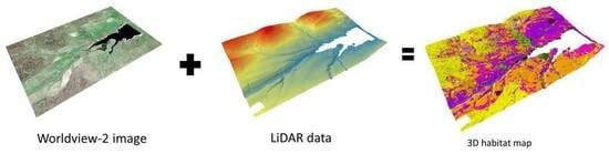
:Progress toward habitat protection goals can effectively be performed using satellite imagery and machine-learning (ML) models at various spatial and temporal scales. In this regard, habitat types and landscape structures can be discriminated against using remote-sensing (RS) datasets. However, most existing research in three-dimensional (3D) habitat mapping primarily relies on same/cross-sensor features like features derived from multibeam Light Detection And Ranging (LiDAR), hydrographic LiDAR, and aerial images, often overlooking the potential benefits of considering multi-sensor data integration. To address this gap, this study introduced a novel approach to creating 3D habitat maps by using high-resolution multispectral images and a LiDAR-derived Digital Surface Model (DSM) coupled with an object-based Random Forest (RF) algorithm. LiDAR-derived products were also used to improve the accuracy of the habitat classification, especially for the habitat classes with similar spectral characteristics but different heights. Two study areas in the United Kingdom (UK) were chosen to explore the accuracy of the developed models. The overall accuracies for the two mentioned study areas were high (91% and 82%), which is indicative of the high potential of the developed RS method for 3D habitat mapping. Overall, it was observed that a combination of high-resolution multispectral imagery and LiDAR data could help the separation of different habitat types and provide reliable 3D information.
1. Introduction
Biodiversity is an important element that influences ecosystem services to humanity. The rate of global biodiversity extinctions has been increasing since humanity’s dominance of the Earth [1,2] as well as growing demands for goods and services [3]. Human activities and climatic change have also caused pressures on global biodiversity due to changes in the structure and function of plants [4,5]. Therefore, effective strategies should be developed to alleviate this massive habitat biodiversity loss [6]. In this regard, information on the extent and spatial distribution of habitat types and their dynamics are needed for different conservation planning activities. Consequently, accurate mapping of habitat types and terrain information are prerequisites for such plans.
Habitat mapping using remote-sensing (RS) techniques has been developing for the last couple of decades [7]. RS is a cost- and time-effective tool that contributes to the natural habitat classification and investigation of landscape changes over wide areas using different datasets, such as multispectral, radar, and Light Detection And Ranging (LiDAR) imagery. RS data are suitable for discriminating different habitat types (e.g., forests, grasslands, and wetlands). Although it is usually not as accurate as field surveys, it has several advantages which make it appealing for habitat classification, especially over vast areas. Former RS studies have mainly focused on the manual interpretation of aerial photographs over small areas. However, aerial photo interpretation is still labor-intensive and time-consuming, and automating the corresponding process is challenging [8]. Therefore, space-borne satellite images with different spatial resolutions are now more popular for habitat mapping [9,10].
Multispectral RS techniques, which use data acquired in visible and infrared parts of the electromagnetic spectrum, are one of the approaches to map and monitor habitat types. Multispectral RS systems use the differences in the reflected radiation from the ground surface associated with the variety of habitat properties to discriminate habitat types [11]. Different habitat types show different reflectance values due to the variation of vegetation properties, structures, and canopies, making it possible to classify and separate them using spectral indices. Most previous studies have investigated the use of medium spatial resolution multispectral data for habitat mapping over large areas [12,13]. However, accurate separation of habitat types requires data with higher spatial resolutions to provide detailed information on the boundary of different habitat types [14,15,16]. Particularly, high-resolution data are more beneficial for fragmented landscapes. Greater levels of detail, such as textural features, which are different for various shapes of plants and canopy levels, can be obtained using high spatial resolution data. However, even with a high-resolution observation, it might be challenging to distinguish some habitat types due to their similar spectral characteristics [11]. Therefore, complementary datasets, such as topographic features, could help differentiate these species [17].
Along with horizontal dimension, vegetation height is also important for habitat classification and three-dimensional (3D) mapping. LiDAR sensors provide measurements of distances (heights) of the top (e.g., canopy height) and the ground surface [8,18,19]. Multiple studies have also used topographic-related features, such as slope, aspect, and roughness, to improve the result of habitat classification. RS datasets are usually used along with machine-learning (ML) models to map habitat types. ML, in integration with mapping techniques, provides automatic pattern detection from the dataset with a variety of independent image features, improving classification accuracies compared to statistical models [20,21]. Some of the ML classification techniques, such as Random Forest (RF), which is a non-parametric classification model, have the advantage of not being relied on assumptions about data distribution, thus showing a high potential for habitat classification [22]. Both pixel-based and object-based (or object-based image analysis) classification approaches have been used for habitat mapping [23,24]. An object-based approach converts pixels with similar spectral information into segments, which will later be the basis of the classification. This technique has shown better performance compared to pixel-based methods [25,26]. For example, ref. [27] showed that the object-based method resulted in a higher accuracy in identifying fragmented grasslands compared to a pixel-based classification technique.
So far, many studies have employed various RS datasets and ML models for habitat classification. For example, ref. [1] explored the use of Unmanned Aerial Vehicle (UAV)–LiDAR point cloud data to extract various topographic and vegetation structure features for forest mapping. In another study, high-resolution RS data were used to produce the Normalised Difference Vegetation Index (NDVI) to map vegetation cover and identify individual tree crowns [28]. Several studies also compared different ML algorithms for identifying specific habitat types and confirmed the high performance of RF classifiers for object-based classification applications [29]. A study conducted by ref. [30] used an object-based RF classification algorithm along with multispectral UAV images to discriminate different tree species in Canada. Ref. [31] also produced a 3D map of coastal habitats using a combination of spectral and height features derived from an airborne topo-bathymetric bi-spectral LiDAR system. This study also analyzed the distinctive attributes of green LiDAR full waveforms to extract habitat-specific features. These extracted features, along with infrared intensities and elevations, were used as input datasets in an RF model. The study assessed the individual contributions of these predictors to the accuracy of the results, aiming to improve the precision of habitat classification in coastal regions. The integration of ML methods with aerial structure from motion photogrammetry for 3D habitat mapping has become a popular approach in recent years [32,33]. For instance, ref. [33] proposed a semi-automated framework for high-resolution benthic habitat classification and 3D mapping. The approach involved utilizing Structure from Motion and Multi-View Stereo (SfM–MVS) algorithms and automated machine-learning classifiers. Benthic habitat classification was produced semi-automatically by extracting various attributes from labeled samples using raw towed video camera image data, which were processed and analyzed by a human annotator.
Although the previous research studies (e.g., ref. [33]) have provided promising solutions for accurate and detailed 3D habitat mapping, they have mainly focused on individual sensor data (e.g., LiDAR or aerial images) or lacked the synergistic integration of multimodal datasets (e.g., active and multispectral passive remote-sensing images). This limitation can hinder their ability to accurately map complex habitats that often exhibit diverse and intricate characteristics. By leveraging the combined power of high-resolution multispectral RS images and LiDAR data, our proposed research aims to bridge this gap and deliver a more comprehensive and precise mapping of habitat structures in the selected study areas. Considering the advantages of remote-sensing and ML models, various habitat types in two different study areas were mapped in this study. To this end, an object-based RF classification algorithm was applied to high-resolution Worldview-2 imagery and LiDAR-derived products. Object-based classification considers spatial context and relationships between neighboring pixels, leading to improved accuracy in identifying and delineating habitat boundaries. Traditional pixel-based approaches used in some previous works may not achieve the same level of precision [23]. The synergy of multispectral satellite imagery and LiDAR data facilitated identifying vegetation structures more accurately. Furthermore, a 3D habitat map for each case study was produced using the classified habitat map and the Digital Surface Model (DSM) derived from LiDAR data.
2. Materials and Methods
2.1. Study Area
The study areas (Figure 1) were parts of two reservoirs of northern England, including Colt Crag reservoir in Northumberland ((55°05′57.6″N, 2°08′42.1″W) and (55°02′48.3″N, 2°03′38.4″W)) and Grassholme reservoir in north Pennines ((54°36′12.4″N 2°12’02.9″W) and (54°34′27.8″N 2°07′24.4″W)). Colt Crag is surrounded by wheatears, meadow pipits, and rough grassland. Different animal species also live in the Grassholme reservoir. This reservoir is primarily used as an angling centre for recreational purposes. In general, these reservoirs have a rich biodiversity of benthal habitats and play a key role in supplying the water for adjacent areas.
2.2. Field Data
Field data were collected by ecological experts using several field surveys with the global positioning system (GPS). The collected data included 28 different land cover classes, such as arable, bare ground, broadleaf woodland, improved grassland, marshy grassland, mixed woodland, scrub, semi-improved acid grassland and calcareous grassland, wet and modified bog, and open water. Among the collected classes, only those which were important for the purpose of this study were considered. The information on the used field samples and their distributions are provided in Table 1 and Figure 1, respectively. As is clear, only a portion of the entire study area (e.g., 5–10%) was surveyed in the field, and most portions were classified using desktop remote-sensing analysis. This considerably reduced costs and time.
2.3. RS Datasets
In this study, Worldview-2 multispectral satellite images were used to discriminate various types of habitats. The images had a spatial resolution of 2 m and contained different spectral bands (e.g., blue, green, red, Near Infrared (NIR), and Red Edge), which are felicitous to distinguish various habitat types specified in this study. It is worth noting that a pan-sharpening algorithm was applied to the Worldview-2 images to improve the spatial resolution to 0.5 m. The Worldview-2 imagery was acquired on 5 May 2018 and 14 May 2018 over the Colt Crag and Grassholme reservoirs, respectively. Furthermore, LiDAR data and their derived features, such as Digital Elevation Model (DEM) and DSM, having one-meter spatial resolution with a vertical accuracy of +/−15 cm RMSE, were employed to improve the classification accuracy and produce the 3D model of the study areas. The UK Department for Environment, Food and Rural Affairs provided the LiDAR products which resulted from the last return LiDAR signal and are accessible through their website at ref. [34]. These products were also resampled to 0.5 m to conform with the satellite images. The LiDAR data for both study areas were obtained on 20 May 2018. Finally, all the layers of the satellite imagery and LiDAR datasets were layer-stacked to be ingested in the classification algorithm.
2.4. Methodology
In this study, 3D habitat mapping was performed using several spectral, textural, and topographic features derived from Worldview-2 and LiDAR data. The workflow of the proposed method is illustrated in Figure 2, and its main steps are discussed in more detail below.
The collected field samples were point-based. These samples were converted to polygons using the high-resolution Worldview-2 images (see Table 1). Finally, all the produced polygons were randomly split into two groups training (50%) and testing (50%). The training data were employed for training the RF classification algorithm, and the test samples were utilized for the statistical accuracy assessment.
Despite the partial pre-processing of Worldview-2 satellite images, geometric and radiometric accuracies, as well as orthorectification, were investigated to make sure they are suitable for producing 3D habitat maps. Pan-sharpening was also applied to the imagery to increase its spatial resolution from 2 m to 0.5 m. The Lidar LiDAR data were pre-processed by a lasnoise from the LAStools extension in ArcGIS to reduce potential negative blunders and possible outliers.
It is widely reported that object-based classification results have a higher classification accuracy compared to a pixel-based method, especially when high-resolution images are available [23,24,35,36,37]. Thus, habitat maps were produced using the object-based image analysis. The first step in an object-based classification method is segmentation. Segmentation involves dividing an image into meaningful and homogeneous regions or segments based on certain characteristics, such as color, texture, and intensity. The goal is to group together pixels that belong to the same object or class while distinguishing them from other objects in the image. In this study, the Worldview-2 multispectral image was first segmented using the multi-resolution segmentation algorithm in the eCognition software package. This algorithm applies relative homogeneity criteria over several resolutions/scales to identify objects.
Obtaining higher mapping accuracy requires integrating spectral and elevation features into the main datasets (e.g., the main spectral bands). Additionally, since object-based image analysis was utilized in this study, various spatial and textural features were used to improve the accuracy of the classification. After evaluating various spectral and structural features, the most efficient attributes were incorporated into the classification system. Table 2 shows the characteristics of the selected features in this study.
After identifying the optimal features, they were ingested into an RF algorithm to classify the input data. RF works by using a collection of decision trees, each of which is comprised of nodes that divide pixels into groups of pixels that are most similar to each other. The nodes are then grouped into habitat classes as the process of division continues, leading to the formation of the final classification map. The algorithm was trained using 50% field samples. The result of this step was the two-dimensional (2D) habitat maps from the study areas.
After producing the 2D habitat maps, two methods were used to evaluate the accuracies of the maps. It was first examined whether the classes visually corresponded to different habitats by analyzing high-resolution imagery. Subsequently, the confusion matrices extracted from the test data (i.e., half of the field samples) were generated to determine the statistical accuracies of the maps.
Finally, the 2D habitat maps and the LiDAR–DSM products were integrated into ArcScene to generate the 3D maps of the study areas.
3. Results and Analysis
Figure 3 shows the classified 2D and 3D habitat maps produced using the object-based RF algorithm and a combination of Worldview-2 and LiDAR data. The accuracy of the 2D maps was first visually assessed by comparison with high-resolution imagery. It was observed that the identified regions matched well with the actual habitat categories of the study areas.
The area of each habitat type in the produced habitat maps was calculated, and the percentage area of each class is illustrated in Figure 4. The most populated habitats in the Colt Crag reservoir were Improved Grassland, Arable, and Semi-improved Acid Grassland, respectively. In the Grassholme reservoir, most areas were covered by Blanket Bog, Wed Modified Bog/Heath, Grassland, and Marshy Grassland, respectively.
The classification accuracies were evaluated statistically, and the independent test data and confusion matrices were used. The classification of the Colt Crag and Grassholme reservoirs resulted in 91% and 82% overall accuracies, respectively. These high classification accuracies showed the high potential of the proposed RS technique for habitat classification. Figure 5 illustrates the producer and user accuracies for each class in the study areas. The accuracy for each individual class was significantly high for most of the habitat categories. In the Colt Crag reservoir, both producer and user accuracies were approximately 100% for the following classes: Bare Ground, Arable, Buildings, Quarry, Water, and Coniferous woodland, indicating that all the samples for these habitat classes were correctly classified. Another reason for the high classification accuracy for the mentioned classes was that these categories have distinct spectral responses in the multispectral satellite images. The Semi-improved Acid Grassland, Wet Modified Bog, and Broadleaved Woodland classes also achieved high accuracy levels. However, the accuracy rates for a few of the classes were relatively low. For instance, the Marshy Grassland class had low accuracy in both study areas. This was mainly because most marshlands were incorrectly classified as Semi-improved grassland.
4. Discussion
The main reason for the incorrect classification of some of the habitat categories was that they share similar ecological and spectral characteristics. Therefore, their spectral data could be assigned to an incorrect class by an ML algorithm. This was particularly observed for subclasses of a habitat type. For instance, it was difficult to discriminate different types of grasslands, where they were interchangeably identified and, consequently, their accuracies were reduced. It should be noted that the accuracy of discriminating grasslands from other habitat types was high. However, there was confusion between the grassland sub-classes. For instance, there were several Semi-improved Calcareous grassland areas that were wrongly classified as the Semi-improved grassland class, and, therefore, the producer accuracy of this class was reduced to 66% in the Colt Crag Reservoir.
LiDAR data were crucial for the classification of the habitat categories that had similar spectral responses but different heights. To illustrate this, the habitat classification of the Colt Crag region was implemented by the sole use of the Worldview-2 satellite image (Figure 6), and the results were compared with those produced from a combination of satellite imagery and LiDAR data (Figure 5a). It was observed that excluding LiDAR data notably decreased the accuracy levels of most classes, especially the elevated classes, such as Scrub woodlands. For example, the producer (user) accuracies of the scrub class decreased from 75% (41%) to 62% (30%) when LiDAR data were not considered in the classification model. Additionally, the averaged producer (user) accuracies of the woodland classes (i.e., Mixed woodland, Broadleaved woodland, and Coniferous woodland) decreased from 89% (95%) to 83% (84%) when LiDAR data were removed from the classification model. In fact, the vertical attribute of LiDAR data served as a crucial discriminator, making LiDAR an invaluable tool in overcoming the limitations of spectral-only approaches. Nonetheless, there were instances where the discrimination of scrubs from other woodlands using LiDAR data faced challenges. In specific cases, the relatively low resolution of the LiDAR data (i.e., 1 m) limited its ability to capture fine-scale variations in vegetation height, leading to reduced accuracy in distinguishing these classes. Despite this limitation, the overall contribution of LiDAR to habitat classification remained substantial. By providing valuable vertical structure information, LiDAR enhanced the precision and reliability of differentiating between various habitat types, especially when height played a pivotal role in delineating distinct ecological zones.
Although DSM was created from LiDAR point cloud data, it can be generated from photogrammetric methods applied to stereo aerial and satellite imagery. Although photogrammetric methods usually have lower accuracy compared to LiDAR-based methods, they are more cost-effective. Therefore, to reduce cost in future studies, it is suggested to use DSM generated from photogrammetric methods [38].
Both the quality and the quantity of the field samples had a significant impact on the classification accuracy of the proposed RF model. In this study, the numbers of field samples for most of the habitat classes were determined to be statistically significant. However, there was a limited number of samples for a few classes yielding low accuracies of the corresponding classes. For example, one of the reasons for the low producer accuracy of the Marshy grassland class could be rooted in the low number of field samples for this class.
One of the limitations in increasing the accuracy of the linear features, such as wet ditches or narrow running water bodies, was the spatial resolution of the RS images. Despite achieving a high-resolution pan-sharpened image with a resolution of 0.5 m in this study, we encountered limitations in effectively discriminating certain linear features from each other. While it is possible that the limitations in discriminating certain linear features can be attributed to the quality of the pan-sharpening method, these issues are primarily caused by the combined effects of the Modulation Transfer Function (MTF) on the edge sharpness of the imagery [39]. This MTF influence results in blurring and reduced contrast of the linear features within the pan-sharpened image. Hence, despite achieving a high-resolution pan-sharpened image, the inherent characteristics of the imaging system, influenced by the MTF, contribute to the challenges in accurately discriminating specific linear features. This might be one of the reasons for the low accuracy of the wet ditches and narrow roads (Hardstanding). If a higher accuracy for linear features is required, higher-resolution images, such as those collected by drones, should be purchased in future works.
It should be noted that the multispectral satellite images (e.g., Worldview-2) cannot see under trees and, thus, it was not possible to detect any features like water bodies and ponds that were beneath the tree canopies. Some RS datasets, such as those acquired by L-band RADAR satellites, could be an effective solution for this problem.
5. Conclusions
RS techniques are highly beneficial for monitoring habitats. Different RS datasets with various spectral, spatial, and temporal characteristics complement each other in habitat mapping applications. The majority of current research on 3D habitat mapping has tended to focus on utilizing features derived from a single sensor or a combination of similar sensors, such as multibeam LiDAR, hydrographic LiDAR, and aerial images. These approaches often overlook the potential advantages of integrating data from multiple sensors. To bridge this gap, our study introduced a novel methodology for generating 3D habitat maps by a combination of Worldview-2 images and LiDAR products in two different study areas using an object-based RF classification method. The image was first segmented into objects, and then each object was assigned to a habitat class. The LiDAR-derived DSM was then used to create 3D habitat maps by adding height information to each pixel of the 2D classified maps. It was concluded that the maps had high classification accuracies, indicating the great potential of the proposed RS method for habitat classification. The results also indicated that a combination of high-resolution multispectral imagery and LiDAR data could provide valid 3D information on habitat classes. LiDAR data were also very helpful in distinguishing the habitat classes with similar spectral responses but different elevations. For example, including LiDAR data increased the averaged producer and user accuracies of the woodland classes by 6% and 11%, respectively.
Author Contributions
Conceptualization, M.A.; methodology, M.A. and S.M.; software, M.A., S.M., F.F. and A.M.; validation, M.A. and S.M.; formal analysis, M.A., S.M., F.F. and A.M.; investigation, M.A., S.M., F.F. and A.M.; resources, M.A.; data curation, M.A. and S.M.; writing—original draft preparation, M.A., S.M., F.F. and A.M.; writing—review and editing, M.A., S.M., F.F., A.M. and S.J.; visualization, F.F. and A.M.; supervision, M.A. and S.J.; funding acquisition, M.A. and S.J. All authors have read and agreed to the published version of the manuscript.
Funding
This research received no external funding.
Data Availability Statement
Data sharing not applicable.
Conflicts of Interest
The authors declare no conflict of interest.
References
- Guo, Q.; Su, Y.; Hu, T.; Zhao, X.; Wu, F.; Li, Y.; Liu, J.; Chen, L.; Xu, G.; Lin, G. An integrated UAV-borne lidar system for 3D habitat mapping in three forest ecosystems across China. Int. J. Remote Sens. 2017, 38, 2954–2972. [Google Scholar] [CrossRef]
- Tittensor, D.P.; Walpole, M.; Hill, S.L.L.; Boyce, D.G.; Britten, G.L.; Burgess, N.D.; Butchart, S.H.M.; Leadley, P.W.; Regan, E.C.; Alkemade, R. A mid-term analysis of progress toward international biodiversity targets. Science 2014, 346, 241–244. [Google Scholar] [CrossRef] [PubMed]
- Foresight. The Future of Food and Farming. Executive Summary; Government Office for Science: London, UK, 2011.
- Jetz, W.; Wilcove, D.S.; Dobson, A.P. Projected impacts of climate and land-use change on the global diversity of birds. PLoS Biol. 2007, 5, e157. [Google Scholar] [CrossRef]
- Sala, O.E.; Stuart Chapin, F.; Armesto, J.J.; Berlow, E.; Bloomfield, J.; Dirzo, R.; Huber-Sanwald, E.; Huenneke, L.F.; Jackson, R.B.; Kinzig, A. Global biodiversity scenarios for the year 2100. Science 2000, 287, 1770–1774. [Google Scholar] [CrossRef]
- Brooks, T.M.; Mittermeier, R.A.; Da Fonseca, G.A.B.; Gerlach, J.; Hoffmann, M.; Lamoreux, J.F.; Mittermeier, C.G.; Pilgrim, J.D.; Rodrigues, A.S.L. Global biodiversity conservation priorities. Science 2006, 313, 58–61. [Google Scholar] [CrossRef]
- Luque, S.; Pettorelli, N.; Vihervaara, P.; Wegmann, M. Improving biodiversity monitoring using satellite remote sensing to provide solutions towards the 2020 conservation targets. Methods Ecol. Evol. 2018, 9, 1784–1786. [Google Scholar] [CrossRef]
- Bergen, K.M.; Goetz, S.J.; Dubayah, R.O.; Henebry, G.M.; Hunsaker, C.T.; Imhoff, M.L.; Nelson, R.F.; Parker, G.G.; Radeloff, V.C. Remote sensing of vegetation 3-D structure for biodiversity and habitat: Review and implications for lidar and radar spaceborne missions. J. Geophys. Res. Biogeosci. 2009, 114. [Google Scholar] [CrossRef]
- Mahdavi, S.; Salehi, B.; Granger, J.; Amani, M.; Brisco, B.; Huang, W. Remote sensing for wetland classification: A comprehensive review. GISci. Remote Sens. 2018, 55, 623–658. [Google Scholar] [CrossRef]
- Amani, M.; Mahdavi, S.; Kakooei, M.; Ghorbanian, A.; Brisco, B.; DeLancey, E.; Toure, S.; Reyes, E.L. Wetland Change Analysis in Alberta, Canada Using Four Decades of Landsat Imagery. IEEE J. Sel. Top. Appl. Earth Obs. Remote Sens. 2021, 14, 10314–10335. [Google Scholar] [CrossRef]
- Amani, M.; Salehi, B.; Mahdavi, S.; Brisco, B. Spectral analysis of wetlands using multi-source optical satellite imagery. ISPRS J. Photogramm. Remote Sens. 2018, 144, 119–136. [Google Scholar] [CrossRef]
- Zhang, R.; Zhou, X.; Ouyang, Z.; Avitabile, V.; Qi, J.; Chen, J.; Giannico, V. Estimating aboveground biomass in subtropical forests of China by integrating multisource remote sensing and ground data. Remote Sens. Environ. 2019, 232, 111341. [Google Scholar] [CrossRef]
- Jin, Y.; Yang, X.; Qiu, J.; Li, J.; Gao, T.; Wu, Q.; Zhao, F.; Ma, H.; Yu, H.; Xu, B. Remote sensing-based biomass estimation and its spatio-temporal variations in temperate grassland, Northern China. Remote Sens. 2014, 6, 1496–1513. [Google Scholar] [CrossRef]
- Zhang, Y.; Shao, Z. Assessing of urban vegetation biomass in combination with LiDAR and high-resolution remote sensing images. Int. J. Remote Sens. 2021, 42, 964–985. [Google Scholar] [CrossRef]
- Hashim, H.; Abd Latif, Z.; Adnan, N.A. Urban vegetation classification with NDVI threshold value method with very high resolution (VHR) Pleiades imagery. Int. Arch. Photogramm. Remote Sens. Spat. Inf. Sci. 2019, 42, 237–240. [Google Scholar] [CrossRef]
- Karlson, M.; Ostwald, M.; Reese, H.; Bazié, H.R.; Tankoano, B. Assessing the potential of multi-seasonal WorldView-2 imagery for mapping West African agroforestry tree species. Int. J. Appl. Earth Obs. Geoinf. 2016, 50, 80–88. [Google Scholar] [CrossRef]
- Joy, S.M.; Reich, R.M.; Reynolds, R.T. A non-parametric, supervised classification of vegetation types on the Kaibab National Forest using decision trees. Int. J. Remote Sens. 2003, 24, 1835–1852. [Google Scholar] [CrossRef]
- Pricope, N.G.; Minei, A.; Halls, J.N.; Chen, C.; Wang, Y. UAS Hyperspatial LiDAR Data Performance in Delineation and Classification across a Gradient of Wetland Types. Drones 2022, 6, 268. [Google Scholar] [CrossRef]
- Wu, G.; You, Y.; Yang, Y.; Cao, J.; Bai, Y.; Zhu, S.; Wu, L.; Wang, W.; Chang, M.; Wang, X. UAV-LiDAR Measurement of Vegetation Canopy Structure Parameters and Their Impact on Land–Air Exchange Simulation Based on Noah-MP Model. Remote Sens. 2022, 14, 2998. [Google Scholar] [CrossRef]
- Rahmanian, S.; Pourghasemi, H.R.; Pouyan, S.; Karami, S. Habitat potential modelling and mapping of Teucrium polium using machine learning techniques. Environ. Monit. Assess. 2021, 193, 1–21. [Google Scholar] [CrossRef]
- Thapa, A.; Wu, R.; Hu, Y.; Nie, Y.; Singh, P.B.; Khatiwada, J.R.; Yan, L.I.; Gu, X.; Wei, F. Predicting the potential distribution of the endangered red panda across its entire range using MaxEnt modeling. Ecol. Evol. 2018, 8, 10542–10554. [Google Scholar] [CrossRef]
- Pham, T.D.; Yokoya, N.; Bui, D.T.; Yoshino, K.; Friess, D.A. Remote sensing approaches for monitoring mangrove species, structure, and biomass: Opportunities and challenges. Remote Sens. 2019, 11, 230. [Google Scholar] [CrossRef]
- Amani, M.; Salehi, B.; Mahdavi, S.; Granger, J.E.; Brisco, B.; Hanson, A. Wetland Classification Using Multi-Source and Multi-Temporal Optical Remote Sensing Data in Newfoundland and Labrador, Canada. Can. J. Remote Sens. 2017, 43, 360–373. [Google Scholar] [CrossRef]
- Mahdavi, S.; Salehi, B.; Amani, M.; Granger, J.E.; Brisco, B.; Huang, W.; Hanson, A. Object-Based Classification of Wetlands in Newfoundland and Labrador Using Multi-Temporal PolSAR Data. Can. J. Remote Sens. 2017, 43, 432–450. [Google Scholar] [CrossRef]
- Benz, U.C.; Hofmann, P.; Willhauck, G.; Lingenfelder, I.; Heynen, M. Multi-resolution, object-oriented fuzzy analysis of remote sensing data for GIS-ready information. ISPRS J. Photogramm. Remote Sens. 2004, 58, 239–258. [Google Scholar] [CrossRef]
- Agarwal, S.; Vailshery, L.S.; Jaganmohan, M.; Nagendra, H. Mapping urban tree species using very high resolution satellite imagery: Comparing pixel-based and object-based approaches. ISPRS Int. J. Geo-Inf. 2013, 2, 220–236. [Google Scholar] [CrossRef]
- Förster, M.; Schmidt, T.; Schuster, C.; Kleinschmit, B. Multi-temporal detection of grassland vegetation with RapidEye imagery and a spectral-temporal library. In Proceedings of the 2012 IEEE International Geoscience and Remote Sensing Symposium, Munich, Germany, 22–27 July 2012; IEEE: Piscataway, NJ, USA, 2012; pp. 4930–4933. [Google Scholar]
- Raciti, S.M.; Hutyra, L.R.; Newell, J.D. Mapping carbon storage in urban trees with multi-source remote sensing data: Relationships between biomass, land use, and demographics in Boston neighborhoods. Sci. Total Environ. 2014, 500, 72–83. [Google Scholar] [CrossRef]
- Wang, D.; Wan, B.; Qiu, P.; Su, Y.; Guo, Q.; Wu, X. Artificial mangrove species mapping using pléiades-1: An evaluation of pixel-based and object-based classifications with selected machine learning algorithms. Remote Sens. 2018, 10, 294. [Google Scholar] [CrossRef]
- Franklin, S.E.; Ahmed, O.S. Deciduous tree species classification using object-based analysis and machine learning with unmanned aerial vehicle multispectral data. Int. J. Remote Sens. 2018, 39, 5236–5245. [Google Scholar] [CrossRef]
- Letard, M.; Collin, A.; Corpetti, T.; Lague, D.; Pastol, Y.; Ekelund, A. Classification of land-water continuum habitats using exclusively airborne topobathymetric LiDAR green waveforms and infrared intensity point clouds. Remote Sens. 2022, 14, 341. [Google Scholar] [CrossRef]
- Leon, J.X.; Roelfsema, C.M.; Saunders, M.I.; Phinn, S.R. Measuring coral reef terrain roughness using ‘Structure-from-Motion’ close-range photogrammetry. Geomorphology 2015, 242, 21–28. [Google Scholar] [CrossRef]
- Mohamed, H.; Nadaoka, K.; Nakamura, T. Towards Benthic Habitat 3D Mapping Using Machine Learning Algorithms and Structures from Motion Photogrammetry. Remote Sens. 2020, 12, 127. [Google Scholar] [CrossRef]
- UK Government. Defra Survey Data. Available online: https://environment.data.gov.uk/DefraDataDownload/?Mode=survey (accessed on 25 September 2020).
- Amani, M.; Salehi, B.; Mahdavi, S.; Granger, J.; Brisco, B. Wetland classification in Newfoundland and Labrador using multi-source SAR and optical data integration. GISci. Remote Sens. 2017, 54, 779–796. [Google Scholar] [CrossRef]
- Fatemighomi, H.S.; Golalizadeh, M.; Amani, M. Object-based hyperspectral image classification using a new latent block model based on hidden Markov random fields. Pattern Anal. Appl. 2022, 25, 467–481. [Google Scholar] [CrossRef]
- Mirmazloumi, S.M.; Kakooei, M.; Mohseni, F.; Ghorbanian, A.; Amani, M.; Crosetto, M.; Monserrat, O. ELULC-10, a 10 m European land use and land cover map using sentinel and landsat data in google earth engine. Remote Sens. 2022, 14, 3041. [Google Scholar] [CrossRef]
- Curcio, A.C.; Peralta, G.; Aranda, M.; Barbero, L. Evaluating the Performance of High Spatial Resolution UAV-Photogrammetry and UAV-LiDAR for Salt Marshes: The Cádiz Bay Study Case. Remote Sens. 2022, 14, 3582. [Google Scholar] [CrossRef]
- Cheng, J.; Bo, Y.; Ji, X. Effect of Modulation Transfer Function on high spatial resolution remote sensing imagery segmentation quality. In Proceedings of the 2012 Second International Workshop on Earth Observation and Remote Sensing Applications, Shanghai, China, 8–11 June 2012; IEEE: Piscataway, NJ, USA, 2012; pp. 149–152. [Google Scholar]
Figure 1.
The study areas and the distribution of in situ data.

Figure 2.
Flowchart of the suggested approach for 3D habitat mapping.

Figure 3.
(a) Worldview-2 multispectral imagery; (b) 2D habitat maps, and (c) 3D habitat maps obtained from the suggested approach for Colt Crag and Grassholme study areas.
Figure 3.
(a) Worldview-2 multispectral imagery; (b) 2D habitat maps, and (c) 3D habitat maps obtained from the suggested approach for Colt Crag and Grassholme study areas.

Figure 4.
The percentage of the area of classified habitats in the (a) Colt Crag and (b) Grassholme reservoirs.
Figure 4.
The percentage of the area of classified habitats in the (a) Colt Crag and (b) Grassholme reservoirs.

Figure 5.
Producer and user accuracies for the habitat classes in the (a) Colt Crag and (b) Grassholme reservoirs using a combination of Worldview-2 satellite image and LiDAR data.
Figure 5.
Producer and user accuracies for the habitat classes in the (a) Colt Crag and (b) Grassholme reservoirs using a combination of Worldview-2 satellite image and LiDAR data.

Figure 6.
Producer and user accuracies for the habitat classes in the Colt Crag reservoir using only Worldview-2 satellite image.
Figure 6.
Producer and user accuracies for the habitat classes in the Colt Crag reservoir using only Worldview-2 satellite image.


Table 1.
Information of the filed samples for different habitat types.
| Study Area | Habitat Class | Area (Ha) |
|---|---|---|
| Colt Crag Reservoir | Arable | 56.28 |
| Bare Ground | 0.22 | |
| Broadleaf Woodland | 10.79 | |
| Building | 0.92 | |
| Coniferous Woodland | 17.39 | |
| Improved Grassland | 41.26 | |
| Marshy Grassland | 4.16 | |
| Mixed Woodland | 12.10 | |
| Open Water | 10.84 | |
| Quarry | 25.01 | |
| Scrub | 0.83 | |
| Semi-improved Acid Grassland | 15.73 | |
| Semi-improved Calcareous Grassland | 10.42 | |
| Wet Modified Bog | 6.02 | |
| Total | 211.96 | |
| Grassholme Reservoir | Blanket bog | 0.52 |
| Bracken | 0.07 | |
| Broadleaf Woodland | 0.14 | |
| Built/Hardstanding | 0.13 | |
| Coniferous Woodland | 0.56 | |
| Disturbed Ground | 0.02 | |
| Grassland | 0.31 | |
| Marshy Grassland | 0.26 | |
| Open Water | 0.07 | |
| Scrub | 0.04 | |
| Wet Modified Bog/Heath (High Calluna Cover) | 0.16 | |
| Total | 2.28 |
Table 2.
The features used in the habitat classifications.
| Feature Type | Source | Utilized Features |
|---|---|---|
| Spectral bands | WorldView-2 | Coastal, Blue, Green, Red, Yellow, Red Edge, Near Infrared (NIR)-1, Near Infrared-2 |
| Ratio and spectral indices | WorldView-2 | |
| Spatial | WorldView-2 | Shape, Size |
| Gray level Co-occurrence Matrix (GLCM) | WorldView-2 | Mean, Variance, Contrast, Dissimilarity, Entropy, and Homogeneity |
| Elevation derivations | LiDAR | Digital Elevation Model, Digital Surface Model, Canopy Height Model, Slope, and Aspect |
Disclaimer/Publisher’s Note: The statements, opinions and data contained in all publications are solely those of the individual author(s) and contributor(s) and not of MDPI and/or the editor(s). MDPI and/or the editor(s) disclaim responsibility for any injury to people or property resulting from any ideas, methods, instructions or products referred to in the content. |
© 2023 by the authors. Licensee MDPI, Basel, Switzerland. This article is an open access article distributed under the terms and conditions of the Creative Commons Attribution (CC BY) license (https://creativecommons.org/licenses/by/4.0/).
Share and Cite
MDPI and ACS Style
Amani, M.; Foroughnia, F.; Moghimi, A.; Mahdavi, S.; Jin, S. Three-Dimensional Mapping of Habitats Using Remote-Sensing Data and Machine-Learning Algorithms. Remote Sens. 2023, 15, 4135. https://doi.org/10.3390/rs15174135
AMA Style
Amani M, Foroughnia F, Moghimi A, Mahdavi S, Jin S. Three-Dimensional Mapping of Habitats Using Remote-Sensing Data and Machine-Learning Algorithms. Remote Sensing. 2023; 15(17):4135. https://doi.org/10.3390/rs15174135
Chicago/Turabian StyleAmani, Meisam, Fatemeh Foroughnia, Armin Moghimi, Sahel Mahdavi, and Shuanggen Jin. 2023. "Three-Dimensional Mapping of Habitats Using Remote-Sensing Data and Machine-Learning Algorithms" Remote Sensing 15, no. 17: 4135. https://doi.org/10.3390/rs15174135
Note that from the first issue of 2016, this journal uses article numbers instead of page numbers. See further details here.