Spreading of Localized Information across an Entire 3D Electrical Resistivity Volume via Constrained EMI Inversion Based on a Realistic Prior Distribution

Abstract

Frequency-domain electromagnetic induction (EMI) methods are commonly used to map vast areas quickly and with minimum logistical efforts. Unfortunately, they are often characterized by a very limited number of frequencies and severe ill-posedness. On the other hand, electrical resistivity tomography (ERT) approaches are usually considered more reliable; for example, they do not require specific calibration procedures and can be easily inverted in 2D/3D. However, ERT surveys are, by far, more demanding and time consuming, allowing for the deployment of a few acquisition lines per day. Ideally, the optimal would be to have the advantages of both approaches: ease of acquisition while keeping robustness and reliability. The present work raises from the necessity to cope with this issue and from the importance of enforcing realistic constraints to the data inversion without being limited to (over)simplistic spatial constraints (for example, characterizing the smooth and/or sharp regularization). Accordingly, the present research demonstrates, by means of synthetic and field data, how the EMI inversion—based on realistic prior models—can be further enhanced by incorporating additional pre-existing pieces of information. While the proposed scheme is quite general, in the specific examples discussed here, these additional pieces of information are, respectively, a reference model along a line across the survey area, and an ERT section. The field EMI results were verified against extensive ground penetrating radar (GPR) measurements and boreholes.

1. Introduction

Geophysical techniques consist of non-invasive sensing methods that are used to infer the physical properties of the subsurface. For example, electrical resistivity tomography (ERT) and electromagnetic induction (EMI) methods are commonly used to retrieve the electrical properties of the investigated medium. As such, they are useful to infer the electrical resistivity (and chargeability) of the subsurface [1,2,3,4]. ERT data are collected using arrays of dozens of electrodes coupled with the soil to ensure galvanic contact with the ground and are, nowadays, regularly inverted using 2D or 3D forward modeling [5,6,7]. On the contrary, EMI measurements can be performed without any physical contact with the surface and can be generally inverted using simple 1D forward modeling [8,9,10]. Due to the need for physical coupling between the electrodes and the ground, ERT surveys are more troublesome than their electromagnetic counterpart. Hence, for example, in the attempt to speed up the acquisition time of typical ERT surveys and be able to cover larger areas quickly, mobile (pseudo-)ERT systems have been developed and tested [11,12,13]. On the other hand, standard EMI equipment is routinely used to assess (quasi-)3D resistivity distribution of extremely vast areas [14,15,16]. In fact, many EMI systems are specifically designed to be operated while mounted on helicopters [17,18].

On the other hand, ERT data do not require any complex procedure for calibration since a test on well-characterized (internal) resistances is sufficient to guarantee measurement consistency and is typically performed automatically using commercial equipment. Unfortunately, this is not true in the case of EMI as, to have absolute calibrated measurements, EMI instruments need to go through a sequence of adjustments [19,20,21,22,23,24,25].

Mapping the measurements collected at the surface into physical properties of the subsurface is, in both the cases of ERT and EMI, an (ill-posed) inverse problem. As will be discussed in detail in the next sections, an appropriate solution to the inverse problem can only be obtained by including additional sources of information. So, additional pieces of information contribute to the selection of the unique and stable physical model of the subsurface, whose ERT and EMI responses are in sufficient agreement with: (i) the geophysical measurements and (ii) the prior knowledge [26]. This prior knowledge might consist of the pre-existing information about the investigated site. The inclusion of additional information into the inversion is, indeed, the essence of regularization theory [27].

Of course, the assessment of the matching between the observed responses and those generated using the inversion models requires a forward modeling calculation. The forward modeling maps the distribution of the physical properties of the subsurface (i.e., the model) to its geophysical responses (i.e., the calculated data). Clearly, for each method, there might exist a variety of possible forward modelling tools characterized by: different dimensionality (1D, 2D, 3D, and even 4D), computational costs, numerical accuracy, and adherence to the actual physical phenomena involved in the investigated processes (e.g., are the induced polarization effects incorporated?). Generally speaking, an inversion scheme based on 3D forward modeling might be more accurate than its 1D version under complex 3D geological settings. However, calculating 3D responses is more computationally demanding. The modeling error that is introduced with approximated forward modeling is, clearly, also an issue in the case of sophisticated 3D forward modeling tools. In fact, even the most advanced 3D ERT forward modeling will be, in any case, just a mere approximation of the real electrical phenomena. Having said this, not considering the inevitable tridimensionality of the subsurface has detrimental effects on the 1D EMI inversions that are (too) often disregarded [28,29]. Despite that, 1D inversion of EMI data is the most common procedure used due to the computational costs and intricacies of 3D EMI forward modeling approaches. In this respect, the practical availability of simple 1D codes for the inversion of large EMI datasets has been addressed, for example, through enforcing some level of spatial coherence between adjacent sounding locations [30,31,32,33]. In these cases, the ill-posedness of the EMI inversion is tackled by introducing regularization terms, acting not only vertically (at the level of each individual sounding) but also laterally, preventing spurious oscillations of the resistivity values between neighboring sounding locations [34]. Over the years, several options have been investigated and implemented as regularization terms (both lateral and vertical). Examples of possible choices for the regularization term that are gaining popularity are those based on the minimum support stabilizer [35,36,37]. These relatively novel regularization strategies promote the selection of solutions characterized by blocky transitions, whereas the most standard approaches (based on the L2 norm) favor, among all the possible solutions compatible with the observations, the one minimizing the spatial variation of the model parameters. To a lesser extent, similar arguments are also valid for the ERT inversion, and, indeed, also in this case, several stabilizer terms have been proposed to tackle its ill-posedness [38,39].

In case of available ancillary information, the same regularization schemes have been used to promote consistency between the inversion of ERT and/or EMI data with the additional sources of knowledge. For example, this is the case of time-lapse inversion, in which the “ancillary” information for the inversion of the dataset at time $t_i$ is brought either by the result from the previous dataset collected at time $t_{i-1}$ (with $t_i>t_{i-1}$) or by the reference model calculated for the initial time $t_0$. Of course, similar strategies also proved their effectiveness when the ancillary data consisted of a few wells or of different kinds of data, e.g., the interfaces from interpreted ground penetrating radar (GPR) or seismic sections [2,40,41,42,43].

Despite the flexibility offered by the newest inversion schemes still based on the minimization of an objective functional [44], probabilistic approaches are becoming more frequent as the required computational resources are more commonly available [45,46]. The great advantage of probabilistic approaches lies in their capability of assessing the uncertainty of the results in a very immediate way and in the possibility to be fed with arbitrary (realistic) prior model distributions [45,47]. In fact, a probabilistic solution consists of an ensemble of models (namely a probabilistic model) rather than of the unique model minimizing the objective functional. From that ensemble of models, the uncertainty of a specific feature can be readily extracted through simply counting the relative occurrence of that feature. On the other hand, the a priori information necessary for the inversion can be provided in the form of samples of the prior distribution [48]. Basically, the prior distribution defines the models to be evaluated as possible solutions to the inverse problem.

In the present research, there was the necessity of testing a strategy based on a realistic prior distribution ensuring that the individual 1D EMI results were compatible with specific expectations about the subsurface (so, not, merely, sparse or smooth vertical resistivity models). In addition, it was crucial to guarantee that, laterally, the solutions were also consistent with the available knowledge about the site; in particular, the present work discusses and compares the effects of taking advantage (as additional constraints during the inversion of 1D EMI data), alternatively, of: (i) a 2D ERT section and (ii) a 2D geological interpretation.

In the following, the results obtained for the experimental dataset were verified and compared against available ground penetrating radar (GPR) measurements and borehole logs.

2. Methods

The goal of the present research was to provide an effective way to include the available prior information, as much as possible, into the inversion of the EMI datasets collected for the (quasi-)3D characterization of the subsurface. Indeed, in most cases, the acquisition of electromagnetic data is performed with, in mind, an idea of the target or with the concurrent availability of different kinds of geophysical measurements [41]. In the present case, at least in the first place, while inverting the EMI data collected over the area under investigation (Figure 1), we assumed the contemporaneous presence of the ERT results along a single acquisition line. Hence, the point here was to migrate the information provided by, for example, the 2D ERT section, across the entire 3D domain of the EMI survey, and, by doing that, to address the inherent ill-posedness of the inversion of EMI data. EMI inversion is extremely ill-posed as a consequence of: (1) the (very) limited number of observations (in our specific case, the used equipment allows for the collection of three frequencies per sounding), (2) the noise in the data, and (3) the nonlinearity of the forward modeling.

In the deterministic framework, the ill-posedness of the data inversion is tackled by minimizing an objective functional. Such a functional consists of a data misfit term and a stabilizing term. The stabilizing term is meant to select, amongst all possible solutions compatible with the data (i.e., the models fitting the observations within the noise level), the unique and stable one that is in accordance with the prior information. Hence, eventually, the picked solution depends on the choice of such a stabilizing term (the regularizer) [49]. Basically, the subset $Q_{\delta }$ of all the possible solutions compatible with the measurements $\mathit{d}$ is defined, within the larger model space $M$ (Figure 2a), by all the models characterized with a data misfit smaller than the expected noise level $\delta$ in the observations. So, with $M$ being the set of all possible models $\mathit{m}$, $Q_{\delta }$ can be defined as $Q_{\delta }=\{\mathit{m}\in M|‖F\left(\mathit{m}\right)-\mathit{d}‖\le \delta \}$, in which $F$ represents the forward modeling. On the other hand, the minimization of the stabilizer term $s$ specifies the correctness subset $M_c$ of the model space. The crucial property of the correctness set is that, within $M_c$, the original inverse problem is well posed (i.e., the solution exists, is unique, and stable). Therefore, the regularized solution can be found in the intersection of $M_c$ and $Q_{\delta }$. A common choice for the regularizer $s$ is $s\left(\mathit{m}\right)=‖\mathit{m}-{\mathit{m}}_{apr}‖$; in this case, the model solution $\mathit{m}$ is selected to fit the data (in fact, ${\mathit{m}\in Q}_{\delta }$) and, at the same time, to be the closest possible to a reference model ${\mathit{m}}_{apr}$ (Figure 2a) [27].

In the present research, the subset of the possible models was not simply defined by the noise level in the data $\delta$ but also as a subset of the realizations of a prior distribution designed accordingly to the available information about the target. Thus, in the proposed approach, the inversion result $\mathit{m}$ was selected by the regularizer $s\left(\mathit{m}\right)$ as the unique and stable solution within the intersection $Q_{\delta }\cap P$, in which $P$ denotes the set of the prior distribution samples (Figure 2b). In all the following proposed tests, the adopted regularizer was chosen as the distance with respect to a reference model: $s\left(\mathit{m}\right)=‖\mathit{m}-{\mathit{m}}_{apr}‖$.

In the present scheme, the benefit—in terms of the uniqueness and stability of the solution—brought by the stabilizer term is unchanged, whereas the difference with the original approach lies in the further adherence of the selected solution to the prior knowledge used to create the samples in $P$. In the present implementation, the set $P$ was populated using the samples that were defined in quite a general manner. In all the tests discussed in the following, we generated each of the $20\times {10}^6$ elements of $P$ as follows:

• Discretizing the 1D resistivity model $\mathit{m}$ in a certain number of layers $N_l$ (in our specific case, we always considered $31$ layers; the interfaces of those layers are at fixed depths; the layers’ thicknesses increase logarithmically with the depth; the top of the bottom half space, i.e., the top of the $31$st layer, —is at $30$ m depth);
• Picking a random number $N_n$ from a homogeneous distribution varying from 3 to $N_{l\_max}<N_l$ (in all the inversions performed in the present paper: $N_{l\_max}$ was always $17$); $N_n$ is the number of layers whose resistivity values are selected randomly. Hence, out of $N_l$, $N_n$ layers have a resistivity value picked from a homogeneous distribution spanning from a minimum and a maximum resistivity value (in our specific case, the resistivity was made varying from $0.5 \mathsf{\Omega }\mathrm{m}$ to ${10}^4 \mathsf{\Omega }\mathrm{m}$);
• Associating each of the remaining ($N_l-N_n$) layers to its specific resistivity value; that resistivity value is set equal to the linear interpolation between the adjacent layers whose resistivity was determined randomly as described in the previous point.

The $N_n$ range depends on the fact that the resistivity of, at least, two layers must be assigned, while too large a number of randomly defined layers (i.e., $N_{l\_max}\simeq N_l$) would generate vertical profiles that are too erratic to be realistic. More generally, in agreement with all the caveats highlighted in the scientific literature (e.g., [50]), the safest—and, in our opinion, the most correct—way to verify the representativeness of the considered prior models with respect to the available knowledge consists of performing an a posteriori check. Our prior knowledge of the site under investigation is based on a single 2D ERT section (as shown in Figure 1 and Figure 3a). Coherently, the effectiveness of our choices concerning the free parameters defining the elements of $P$ has been checked via the systematic comparison of the resistivity distribution that was obtained through inverting the ERT measurements (Figure 3a) against the best-fitting selection of the samples of the prior distribution to be used to invert the EMI data (Figure 3b).

Indeed, the representativeness of the samples of the prior distribution not only concerns the quality of the models but also the numerosity of the realizations. So, a reasonable fitting of the resistivity section shown in Figure 3a demonstrates that the characteristics of the samples match those of the target and that their numerosity is also sufficient. In our specific case, the prior distribution was defined via $20\times {10}^6$ elements, which are likely far more than what would be considered strictly necessary.

Concerning the depth range defining the prior models, as in any other inversion scheme, it must be defined accordingly to the frequencies used. In particular, the use of discretization with a too small number of layers and/or with a limited maximum depth should be avoided since they may lead to unsatisfactory data fitting and/or unwanted abrupt resistivity variations caused by insufficient parameterization. On the contrary, over-parameterizing the models does not have any negative effects other than the increased computational costs of the prior distribution calculation. Actually, having the prior models with a large number of layers and significant depth (which in our specific case was $30\mathrm{m}$) allowed for the present analysis to focus on the effects of the constraint and the chosen prior rather than on those induced by the number of layers and/or the limited depths.

Once the prior models have been generated, the corresponding geophysical responses need to be calculated by making use of the available forward modeling approximation: in our specific case, $F$ (see, for example, [51,52,53]). So, while the set of the prior models $P$ belongs to $M$ (Figure 2b), it is also necessary to calculate its image in $D$, i.e., $F\left(P\right)$. The elements of $F\left(P\right)$ can be immediately compared against the observations $\mathit{d}$.

In a broader perspective, the rationale behind the construction of the prior is rather similar to the way the training datasets are created in the context of the machine learning approaches [54]; also in those cases, the set of couples $\left(\mathit{m},\mathit{d}\right)$, consisting of the prior models and the corresponding electromagnetic responses, and forming the training dataset, are generated in accordance with the stationary assumption. Hence, the couples in the training dataset (as well as of the prior ensemble $P$ and the associated image $F\left(P\right)$—Figure 2b) need to be independent and identically distributed (IID) random variables [55].

After $F\left(P\right)$ is calculated, it is possible to determine the models associated with the data belonging to the intersection $F\left(P\right)\cap {F(Q}_{\delta })$ between the images in $D$ of the subsets of the model space $P$ and $Q_{\delta }$, meaning the corresponding subset $P\cap Q_{\delta }\subset M$ can be easily defined. Finally, the model $\mathit{m}\in P\cap Q_{\delta }$ minimizing the regularizer $s\left(\mathit{m}\right)$ is selected as the solution to the inverse problem.

The proposed approach can be considered an extension of the spatially constrained inversion [19,31]. However, in the proposed scheme, the vertical regularization was not limited to a simple request for maximum smoothness. Indeed, in the present approach, the spatial coherence in the vertical direction was provided by being an element of the prior ensemble $P$. Thus, the resemblance with the spatially constrained inversion was merely limited to the way in which the lateral bindings were formalized, paving the way for the reconstruction of much more complex geological features (compatible with the prior information).

It might be worth mentioning that, in the proposed scheme, the EMI soundings next to the ERT section (or, in general, to any other available source of prior information) were directly conditioned using the resistivity values of the ERT section itself (e.g., Figure 3a), whereas the EMI soundings that were further distant from the ERT section were constrained to the adjacent EMI soundings (towards the original constraint, i.e., the ERT section). Hence, the influence of the original information derived directly from the ERT section competed with the conditioning supplied by the EMI measurements and gradually lost its intensity as a result. This is consistent with the fact that far from the ERT section, we expected a less significant resemblance between the electrical and the electromagnetic results.

From a computational point of view, the proposed approach was only apparently expensive. In the reality, for similar geological settings, the elements of $P$ can be pre-calculated and, since the forward response is independent for each 1D model, this procedure is massively parallelizable. In addition, all the difficulties connected with the minimization of the objective functional of the standard deterministic approaches (for example, the selection of Tikhonov’s parameter [56]) are automatically removed: the problem reduces to the simple calculation of the norm of the model distance in $s\left(\mathit{m}\right)$.

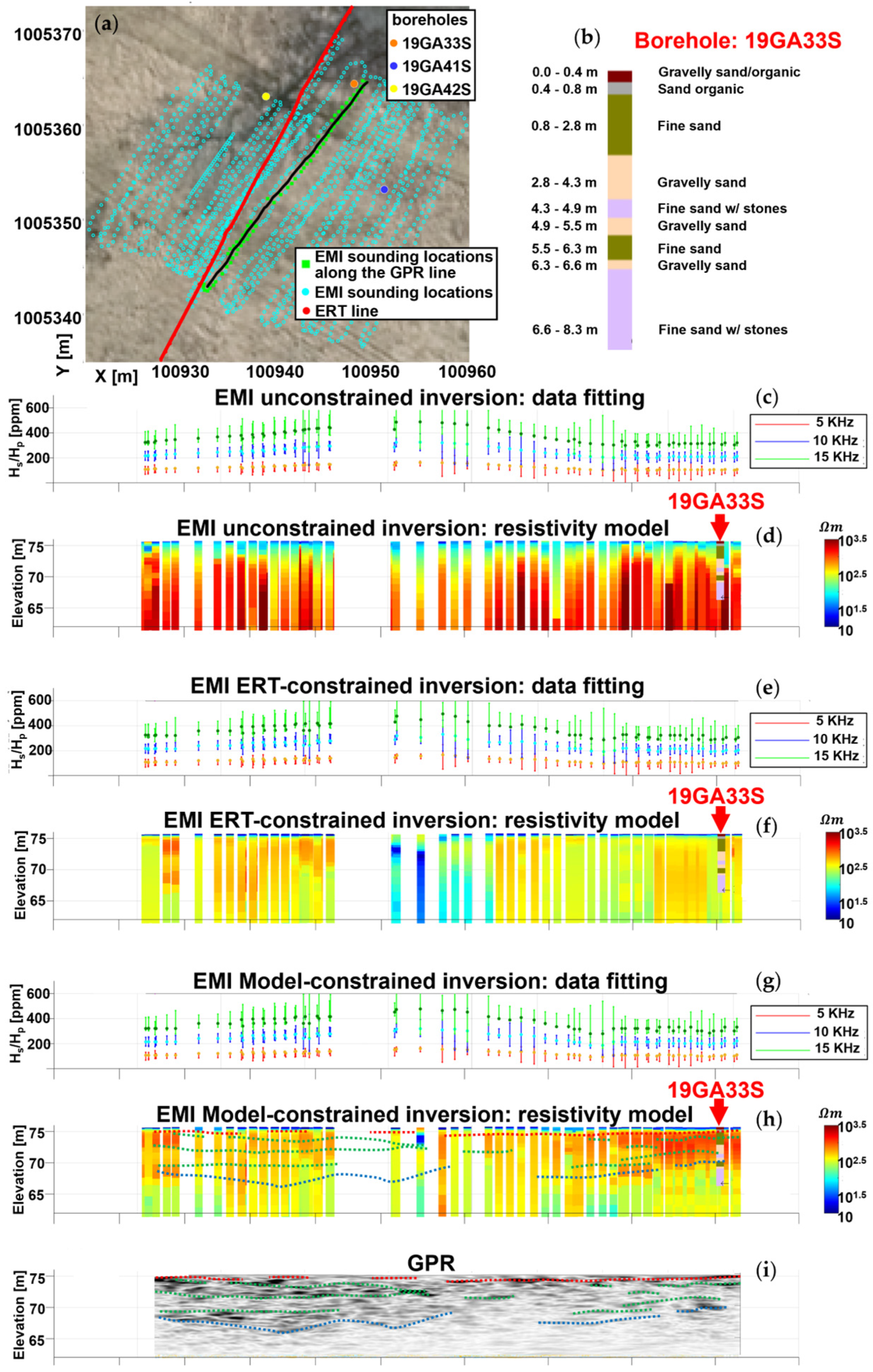
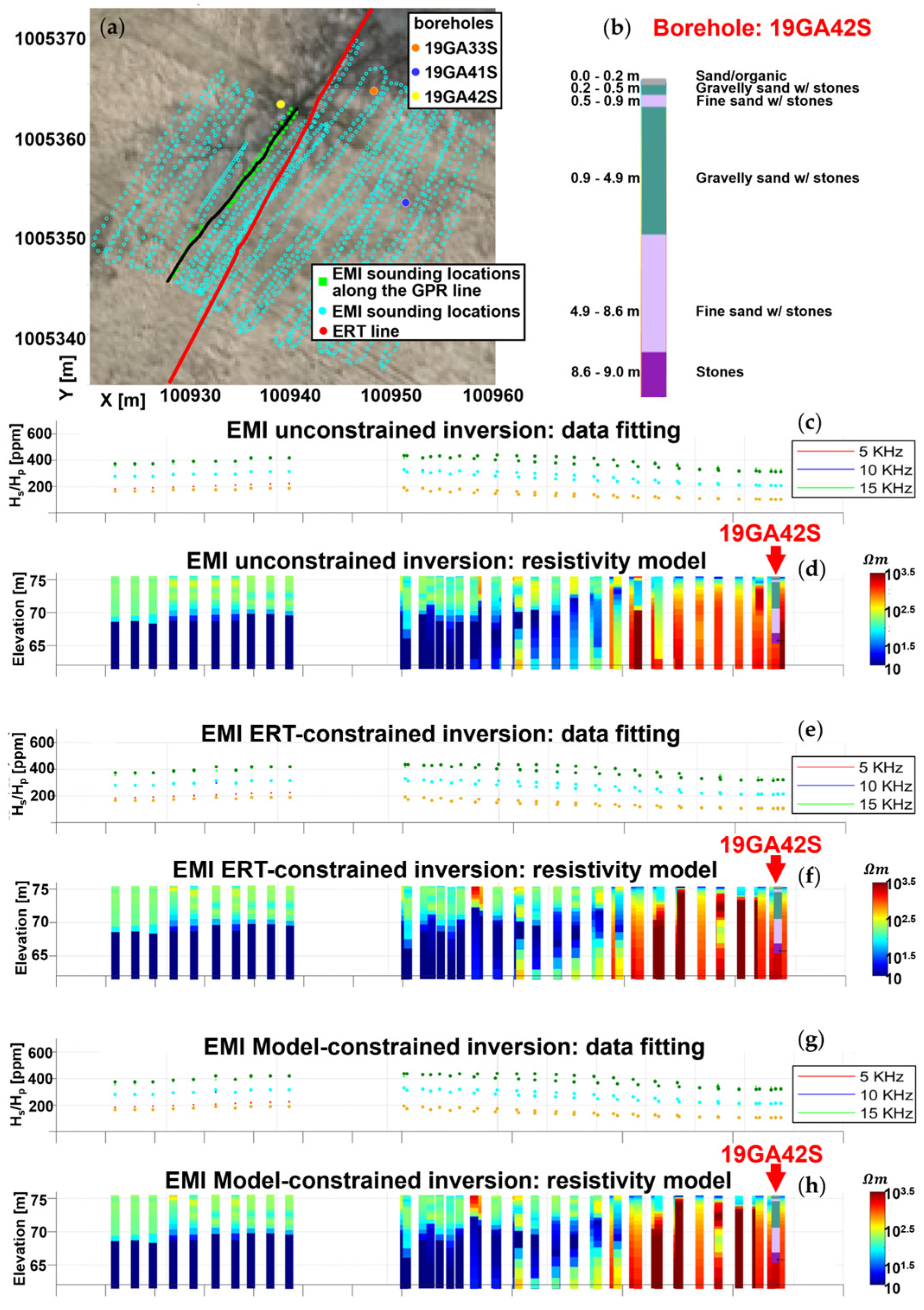
3. Experimental Data

The field observations (Figure 1) discussed in the rest of this study have been collected in the vicinity of Osby, Sweden. The investigated area is characterized by post-glacial fluvial sediments down to about 30–40 m deep. The geology is complex with heterogeneous materials with different grain sizes (from clay to cobbles) and alternating layers (mainly dominated by sand and gravel). In some areas, the top meter mostly comprises organic material or filling gravely deposits. In addition, the test site is distinguished by the presence of a supposedly non-metallic pipe embedded in a sequence of sandy and gravelly layers. The synthetic test was designed to mimic similar features as the experimental case.

In short, the field data consisted of:

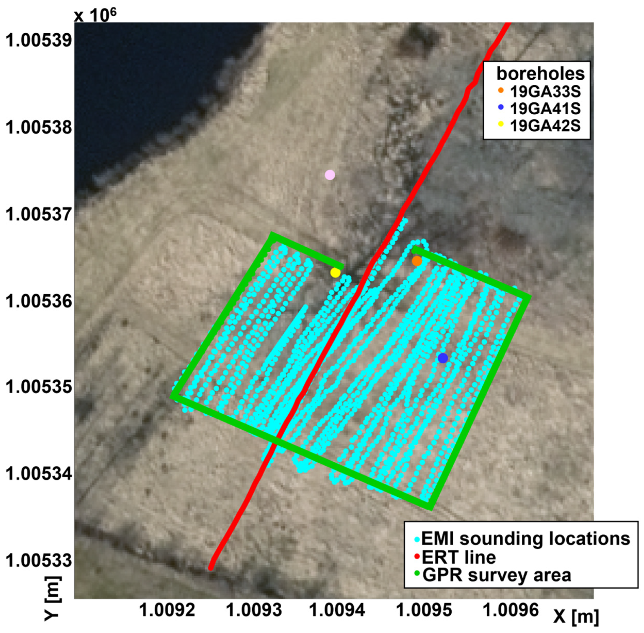
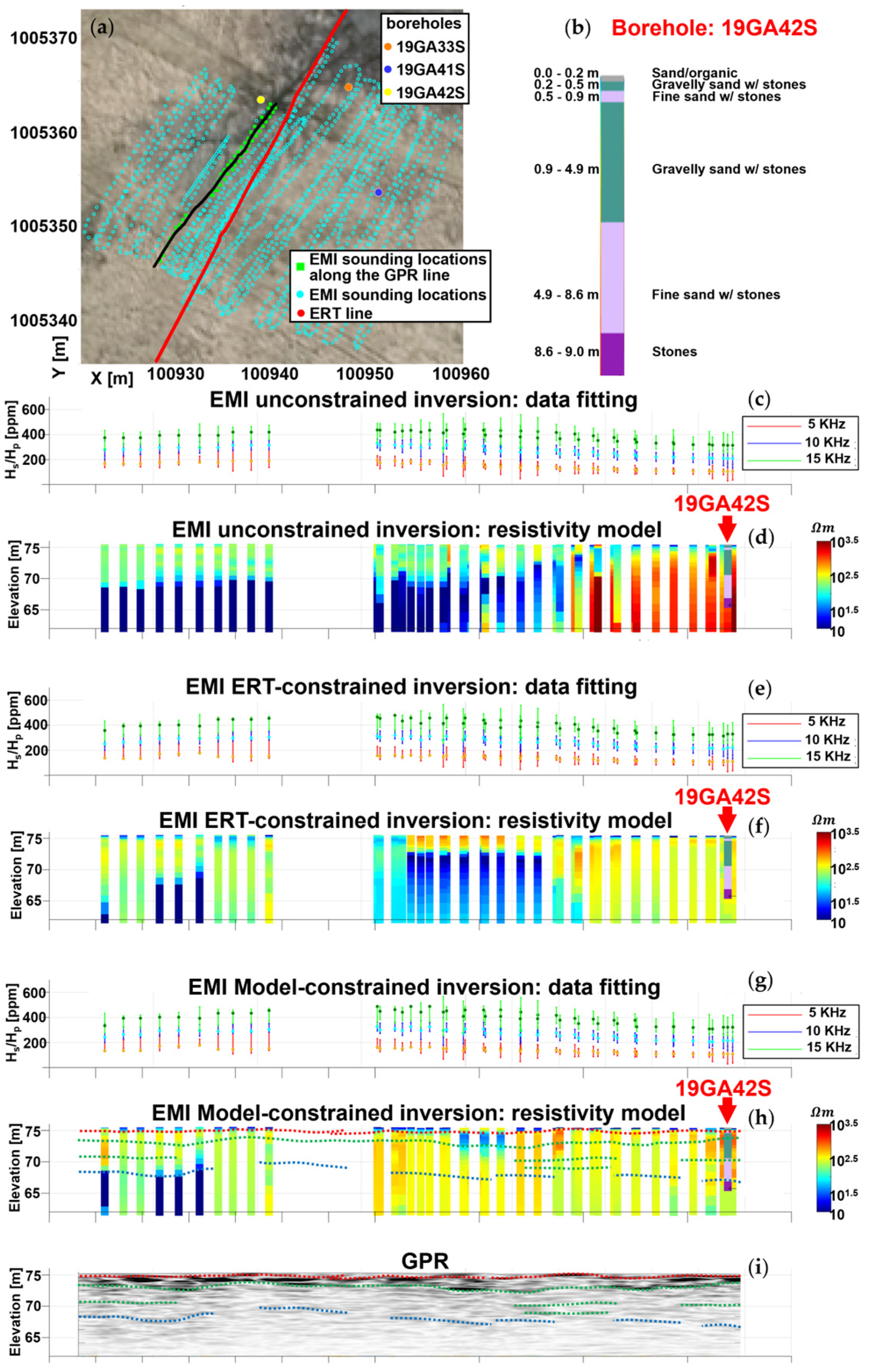
• The EMI measurements collected using a Profiler EMP-400 manufactured by GSSI [57,58,59] with three operative frequencies: $5 \mathrm{K}\mathrm{H}\mathrm{z}$, $10 \mathrm{K}\mathrm{H}\mathrm{z}$, and $15 \mathrm{K}\mathrm{H}\mathrm{z}$. The EMI equipment was calibrated on-site following the procedure outlined by the manufacturer. The sounding locations (1550 soundings with 3 frequencies each) were depicted as light blue dots in Figure 1 over an area of approximately $20\mathrm{m}\times 30\mathrm{m}$.
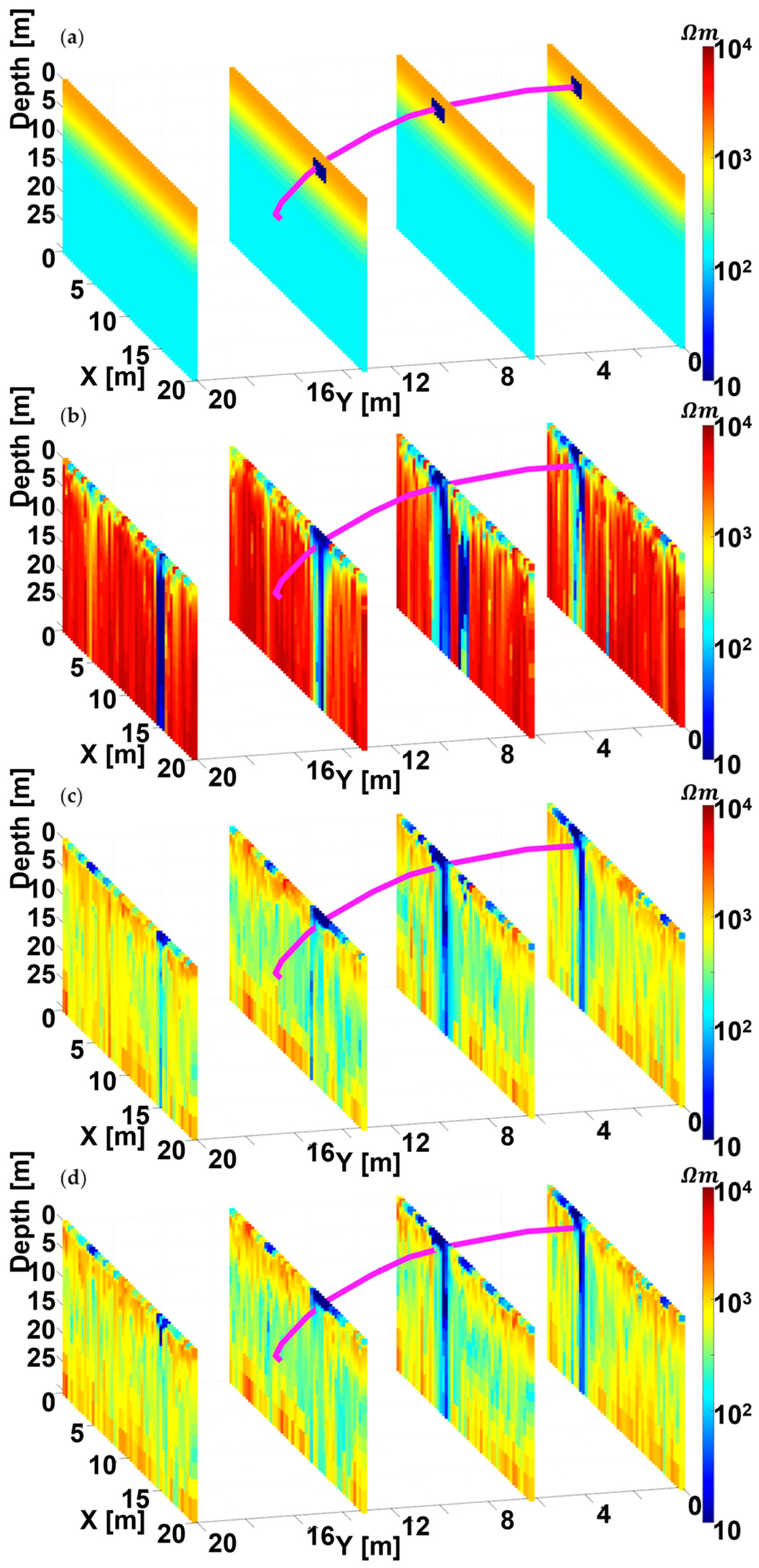
• One ERT acquisition line crossing, in the middle, the entire EMI survey area (red line in Figure 1). The ERT survey was performed using a Terrameter LS2 instrument (GuidelineGeo), with 81 electrodes spaced 1 m. The contact electrical resistance was less than 1 KΩ, and the 1603 data points obtained were acquired via a gradient nested array. The inversion of the ERT section, performed with the software pyGIMLi [60], is shown in Figure 3a (only the portion of the profile included in the area investigated with the EMI method is visible). In Figure 3a, at around $X=29 \mathrm{m}$, the presence of the pipe is clearly recognizable as a very conductive spot.
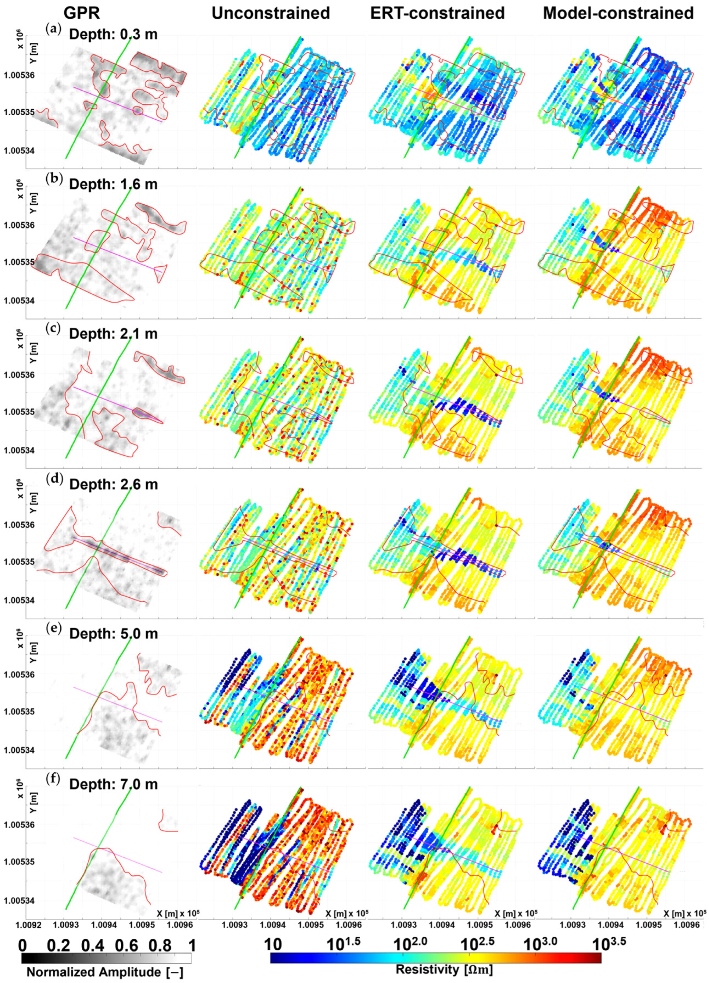
• Several GPR profiles in a $1\mathrm{m}$ grid, overlapping the area of the EMI survey. GPR data were acquired using an ImpulseRadar CO1760 instrument. The GPR results were obtained through processing the 170 MHz signal following the standard workflow consisting of: band-pass filtering, time-zero correction, ringing removal via FK-filtering, and application of the same gain to all sections. The processing output was then Kirchhoff migrated and the signal’s envelope was subsequently interpolated over the 3D volume. For the time-depth conversion, a homogeneous velocity was considered across the entire survey volume; the used velocity value was 95 m/μs. This specific value was estimated by fitting and averaging several diffraction hyperbolas. The reliability of the assumed velocity was verified through the migration and its value was deemed to be compatible with the freshwater-saturated sand/gravel environments [61] characterizing the field site.

In addition to the EMI, ERT, and GPR measurements, a few boreholes were also available in the surroundings of the Osby site. Their locations are shown in Figure 1 as yellow, orange, and blue large dots [62]. The borehole logs were characterized using the sequences of the alternating sand, gravel, and stone layers.

As shown later in the text, the concurrent availability of the boreholes and the GPR data allowed for the interpretation of the radar reflections associated with some of the interfaces intercepted by the boreholes. The information from the radar and borehole logs was used to validate the markedly different results obtained via the applied inversion schemes. In particular, it is worth stressing that, in the acquisition area, the water table is between $1\mathrm{m}$ and $2\mathrm{m}$ deep and that the groundwater consisted of fresh water (the field is a few tens of meters from a river). Hence, we expected a significant correspondence between the lithological interfaces delineated by the borehole logs and the transitions in the subsurface electrical properties inferred from the EMI data.

4. Results

This section discusses the results of applying the schemes presented in the Section 2 to both synthetic and field datasets.

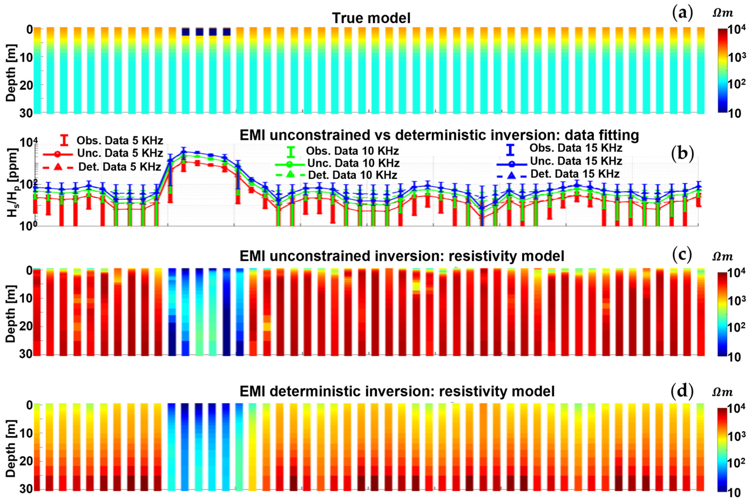
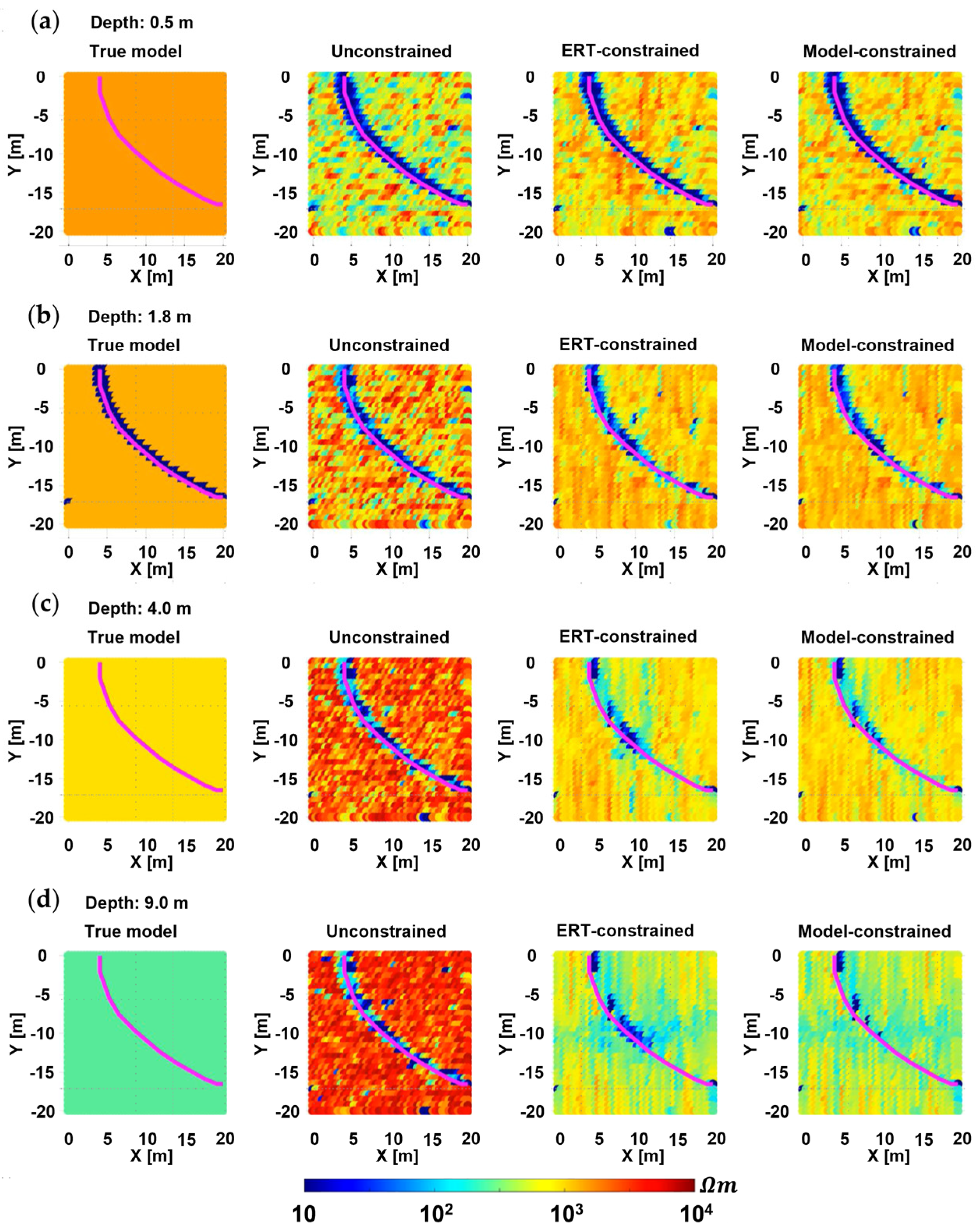
4.1. Synthetic Test

For the synthetic dataset, we used the measurements simulated for the resistivity distribution displayed in Figure 4a. The simulated data consisted of the EMI measurements (of only the quadrature components) calculated for the three frequencies: $5 \mathrm{K}\mathrm{H}\mathrm{z}$, $10 \mathrm{K}\mathrm{H}\mathrm{z}$, and $15 \mathrm{K}\mathrm{H}\mathrm{z}$, using a 1D forward modeling approximation. Thus, differently from the field test (discussed in the following section): (i) no 3D effects were present in the synthetic data, and (ii) the 1D resistivity model associated with each of the sounding locations was considered separately.

The resistivity model (Figure 4a) consists of a relatively low resistivity half-space, topped with a formation characterized by a thickness of around $10 \mathrm{m}$ and a smoothly increasing resistivity from the bottom to the surface. Additionally, a homogeneous rectangular conductive body was embedded into the shallow formation: it is supposed to mimic the presence of a pipe and the effects of the associated excavation trench; its trajectory has been represented in Figure 4a as a solid purple line.

Prior to the inversion, some noise was added to the original (noise-free) synthetic data (vertical bars in Figure 5b,d,f). In particular, the data to be inverted were contaminated with Gaussian noise equal to 5% of each individual measurement, which was added on top of further Gaussian coherent noise. The coherent noise was generated through perturbing the true resistivity models; the model perturbation was selected to be Gaussian with a standard deviation equal to 75% of the resistivity values of each layer. However, in the attempt to follow the conventional processing procedure, which is generally utilized when dealing with field data, the actual noise estimation for the synthetic data was, on average: 110% for the $5 \mathrm{K}\mathrm{H}\mathrm{z}$ channel, 75% for the $10 \mathrm{K}\mathrm{H}\mathrm{z}$ measurements, and 59% for the $15 \mathrm{K}\mathrm{H}\mathrm{z}$ data, respectively. These estimations were assessed through measuring, sounding-by-sounding, the mismatch between the filtered data and the actual measurements. The used filter was a simple average over a moving window four-soundings wide. Clearly, the data that were subsequently inverted were the filtered ones.

By performing the unconstrained inversion (Figure 4b), the EMI soundings were inverted individually, relying uniquely on the prior information brought by $P$. So, in this case, there was no lateral coherence enforced by any reference model ${\mathit{m}}_{apr}$. Still, since the solution is an essential element of $P$, the vertical resistivity distribution cannot be arbitrary. In short, in the unconstrained inversion, the selected solution was not constrained with any lateral bonds (i.e., there was no regularizer $s\left(\mathit{m}\right)$) but it was still conditioned in the vertical direction by the geostatistical information used to generate the samples of $P$. The unconstrained inversion (Figure 4b and Figure 5b,c) fitted the noisy data extremely well and was deemed to be capable of detecting the pipe. However, the unconstrained solution was not able to reconstruct the conductive target nor the vertical resistivity variations across the volume.

It might be worth noticing that the footprint in the data of the conductive pipeline (Figure 5b) was larger than the lateral extension of the conductive inclusion (Figure 5a). Consistently, the retrieved conductive anomaly (Figure 5c) was broader than the actual simulated pipeline width. This larger footprint was deemed to originate from the way the synthetic (noisy) data have been handled. In fact, as discussed before, the original noisy data were laterally averaged to increase their robustness. At the same time, the spatial filtering resulted in a smoothing (and smearing) of the anomaly effect in the data.

The unconstrained inversion was not able to properly reconstruct the pipe and the layering of the background. To cope with this difficulty, one possibility was to spread the local information—originated, for example, by some boreholes, other geophysical measurements, or prior geological observations/expectations—across the EMI survey area.

In the present work, we explored the possibility of using the additional prior information from a single 2D section crossing the volume of the investigated subsurface:

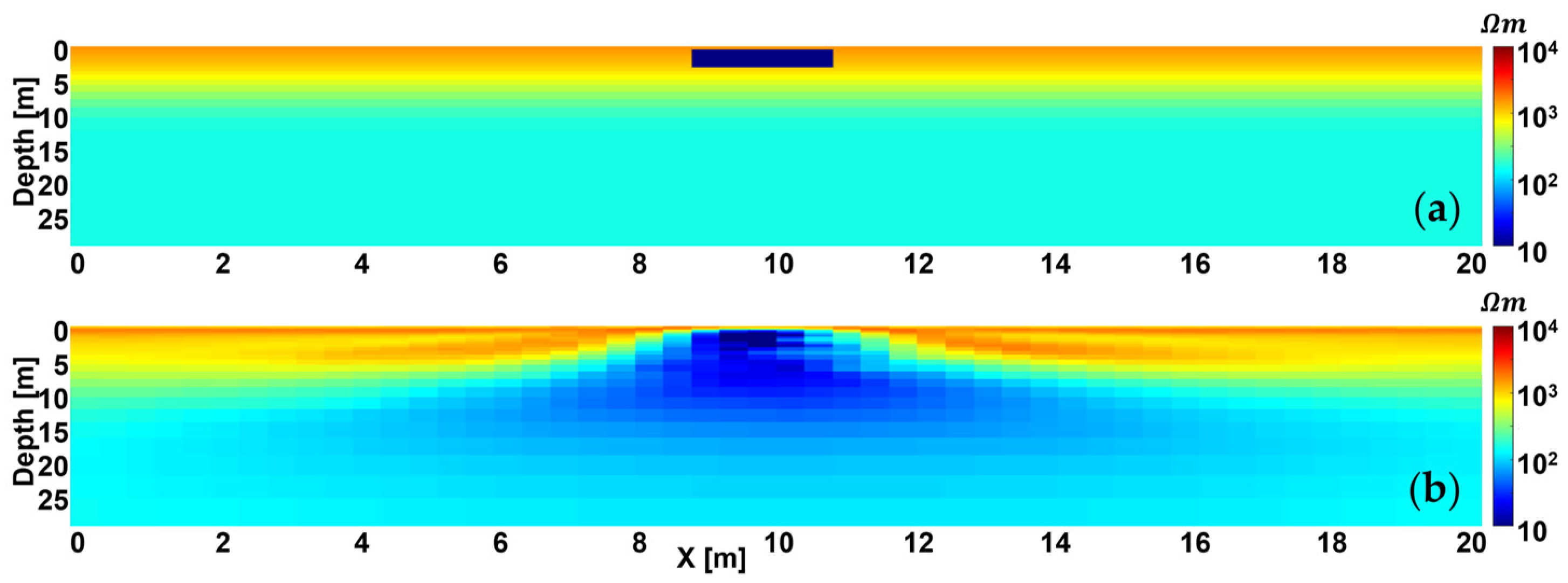
• In the first test, the 2D section consisted of the result of a 2D ERT inversion (Figure 6b). Specifically, the 2D ERT response of the true resistivity model section at $Y=10 \mathrm{m}$ (Figure 6a) was first calculated and then inverted. Then, the resulting ERT section (Figure 6b) at that location was used to spatially constrain the EMI inversion.
• In the second test, the 2D section consisted of a slice (still at $Y=10\mathrm{m}$) of the true resistivity model (Figure 6a).

Figure 4c,d show the EMI results obtained through constraining the inversion of each sounding to the adjacent one and taking into account the two different hypotheses concerning the availability of ancillary data: (i) the 2D ERT section in the middle of the investigated volume, or (ii) a 2D section of the true model. The associated data fitting has been displayed in Figure 5d–g. It is important to stress that the data fitting level for all the reconstructions (e.g., Figure 5b,d,f) was extremely similar and, in all three cases, the associated ${\chi }^2$ value was around $0.1$ (indicating that the data were fitted well below the noise level).

In both cases (cf., for example, Figure 4c,d), the new constrained results outperform the unconstrained inversion in Figure 4b in terms of the correctness of the resistivity values. In fact, the constrained inversions can infer the true resistivity values reasonably well to the depth of around $15\mathrm{m}$. In fact, it does not really matter what kind of ancillary information is used. Indeed, regardless of whether the ERT section or the true model is utilized in the constrained inversions, the resistive top layer, as well as the more conductive half-space, are reconstructed properly (at least down to the depth where a significant sensitivity of the data to the model parameters is to be expected). Unsurprisingly, the inversion relying on the true model section (Figure 4d and Figure 5g) were able to better retrieve the limited thickness of the pipeline. This is particularly evident in Figure 7, in which the horizontal sections of the true resistivity model at different depths (panels in the left column) are compared against the corresponding horizontal slices of the 3D resistivity volumes obtained with the different constraints.

The horizontal slices at $4.0 \mathrm{m}$ (Figure 7c) and $9.0 \mathrm{m}$ (Figure 7d) depth show that: (i) the constraints provide more information to reconstruct the background and the pipe path better, and that (ii) the inversion constrained by the true model section at Y = 10 m (Figure 6a) can overcome the shielding effect of the shallow conductive anomaly that is preventing the retrieval of the more resistive layers below the pipeline in the unconstrained result.

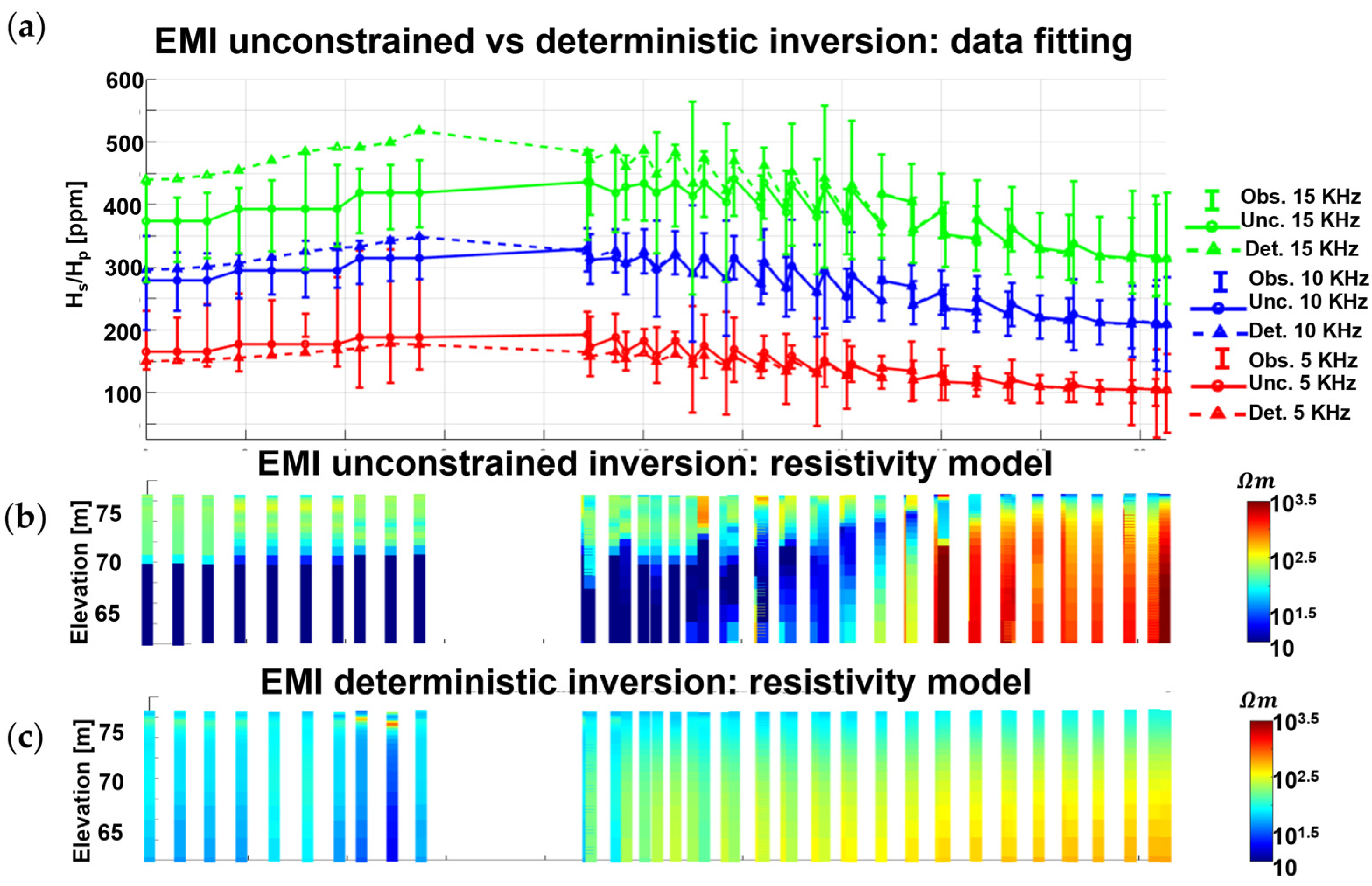
4.2. Field Test

In the field test, the three EMI inversion results are displayed in Figure 8. Similar to the synthetic test, the unconstrained result—relying simply on the data and the information provided by the prior distribution (Figure 8a)—appears to be more resistive than the constrained inversions (Figure 8b,c), which instead incorporate the information from the 2D ERT section and its interpretation, respectively. In Figure 8 and Figure 9, it is clear how the introduction of ancillary information (either via the ERT section or its interpretation) makes the results more spatially consistent, significantly reducing the erratic variation between the different adjacent 1D models.

Moreover, Figure 9 compares, at different depths: (i) the horizontal slices of the envelope of the GPR reflections, and (ii) the corresponding slices of the EMI volumes obtained via different constraining strategies (but with the same prior model distribution). Such a comparison confirms the effectiveness of the schemes incorporating the ancillary information. For example, Figure 9c,d show that the EMI data can easily detect the relatively conductive anomaly connected with the presence of the pipeline highlighted by the GPR sections at $2.1\mathrm{m}$ and $2.6\mathrm{m}$ depths. The spatial coherence and consistency with the GPR results are not limited to the reconstruction of the pipeline. Incorporating the additional ancillary information leads to the retrieval of homogeneous domains in the EMI results that are in good agreement with the (independently obtained) GPR results (e.g.,: Figure 9d,e). Similarly to the synthetic test, the inversion based on the interpretation of the 2D ERT vertical section seems to provide a more realistic reconstruction of the limited size of the pipeline, and of the other surrounding features (e.g., at $5\mathrm{m}$ depth).

Alongside the verification against the GPR data, vertical sections of the inferred resistivity volumes have also been compared with the available borehole logs (Figure 1). In Figure 10, the vertical sections of the different 3D EMI inversions are shown together with the corresponding GPR vertical cross-section and the stratigraphy associated with the nearest borehole (19GA42S). The significant differences between these vertical resistivity sections highlight, one more time, the importance of incorporating the proper ancillary information into the inversion: even the constrained results are quite distinctive (Figure 10f,h). And this variability occurs despite the observations being fitted in all the cases equally well (Figure 10c,e,g). Moreover, the Model-constrained inversion appears to be in better agreement: (i) with the GPR section (Figure 10i), and (ii) with the borehole log description. For example, concerning the borehole stratigraphy, not only can the EMI results match the conductive shallow layers, but the Model-constrained inversion can also correctly locate the interface at $8.6\mathrm{m}$ depth (with around $67\mathrm{m}$ in elevation), as evident in the log (Figure 10b).

Similar conclusions can also be drawn by checking the other boreholes. For example (analogously to Figure 10), Figure 11 shows the results related to boreholes 19GA33S. In this case, the different EMI inversions were also found to display quite different resistivity distributions.

The ERT-constrained result is characterized (consistently with the constraint, as shown in Figure 3a) by a deep conductive anomaly around the center of the section, whereas the data are equally well-fitted by the shallower and more compact conductive anomaly of the Model-constrained result. This is, again, in accordance with the provided ancillary information characterized, in this case, by a blocky square conductive body embedded in a laterally homogeneous background (similar to the distribution displayed in Figure 6a).

Furthermore, the features in Figure 11h were found to match better with the strongest radar reflections (Figure 11i); the reconstruction based on the interpretation of the ERT (Figure 11h) was able to detect the interface on the top of the fine sand layer at $5.5 \mathrm{m}$ depth (Figure 11b) more effectively compared to the other two inversions. This interface was evident in the borehole stratigraphy and produced a strong reflection in the GPR section.

In the proposed inversion scheme, it must be noted that the smaller the noise level assumed in the data, the less intense the impact of the constraint. In other words, if the quality of the observations is high, the resistivity reconstruction is mainly based on the measurements and the prior distribution samples (in principle, with no need for additional inputs from the ancillary data). This can be further and more explicitly shown by performing the ERT- and Model-constrained inversions assuming an extremely low uncertainty in the data to be inverted. In this respect, Figure 12 shows the resistivity sections in Figure 10, but now calculated for an assumed noise level equal to $0.01$% of the original one. Coherently, Figure 12f,h display identical resistivity sections that are almost equal to the unconstrained result shown in Figure 11d.

5. Discussion

The present research discusses an inversion scheme to be applied to EMI data that relies on the concurrent use:

• Of an arbitrarily complex prior distribution (used for conditioning the solution along the vertical direction, i.e., sounding-by-sounding).
• Of the ancillary available information in the form of ERT cross-sections or in the form of the interpretation of the geoelectrical cross-sections (which are useful for enforcing lateral consistency across the final 3D resistivity volume).

From our results, it is clear how the inversion of EMI data is severely non-unique (e.g., Figure 10d,f,h). It is also evident that the ability to formalize the available information both via the prior distribution samples and by means of the reference models (e.g., consisting of the 1D models associated with the ERT result) is crucial. Indeed, the use of ancillary data as a reference model allows migrating the information from a single ERT section (or its interpretation) to the entire volume investigated via the EMI acquisition (e.g., Figure 9). In addition, the availability of ancillary information allows for an effective check of the consistency of the prior model distribution against the available pre-existing data (Figure 3).

The capabilities of the proposed approach are clear when the 3D EMI results were compared against the geological descriptions of the borehole logs. For instance, Figure 11d,f,h present quite different resistivity distributions in the neighborhood of the borehole, despite their equally good fitting of the measurements. This ambiguity is related to the ill-posedness of the original problem (which was tackled, in the three schemes, via the inclusion of three different prior information types). To some extent, this ambiguity is also ascribable to the low sensitivity of the data to relatively high resistivities (in this respect, e.g., cf. [63,64]). In fact, very different high-resistivity values may not correspond to significantly different responses. In the specific case of Figure 10 and Figure 11, this problem was exacerbated by the resistive anomalies nearby the wells being below a shallow conductive layer that highly reduces the depth of investigation (or, in other words, the integrated sensitivity) [44,65]. Consistently, due to the limited depth of investigation, no experienced interpreter would rely on these results at depth unless they were corroborated with ancillary observations. The advantage of these proposed constrained schemes is that these ancillary observations were integrated into the inversion itself ab initio.

Concerning the inherent ambiguity of the EMI inversion, it might be relevant to compare the results of the proposed approaches against those inferred via a well-known open-source software [34]. Even though this comparison was not the main focus of this study, it can be helpful to appreciate the differences with respect to a more usual deterministic approach. For this reason, the details of this comparison have been discussed in Appendix A, in which the unconstrained inversions were inspected together with an L2-norm inversion for both the synthetic and field datasets.

In addition, the lithological interfaces in the borehole logs were confirmed, not only by the EMI inversions, but, independently, also by the GPR reflections. Based on the vertical GPR sections considered in Figure 10i and Figure 11i, a few reflectors have been interpreted in accordance with the available borehole logs and the spatial coherence of the reflected signals. These reflectors were shown, in this study, as colored dashed lines: red lines represented the shallower reflectors, blue lines denoted the deepest reflections visible in the radargram, while the green lines indicated several identifiable anomalies due to the heterogeneity of the sedimentary deposits with variable grain size distributions. To make the subsequent comparisons easier, the same GPR interpretations were copied on the Model-constrained results in Figure 10h and Figure 11h, respectively. It is evident that several GPR reflections were caused by geological boundaries that were also visible in the borehole logs and in the EMI results. For example, the dashed blue line in Figure 10i, associated with the reflection of the top of the stones layer, matched well with the changes in resistivity both at the borehole location and, in general, with the increase in conductivity at the bottom of the section (Figure 10h). Moreover, the shallow conductive layer in Figure 10h matched well with the organic matter found in the boreholes. This organic matter extends across the entire area (red dashed line interpreted from the GPR), and we can also see some evidence of this layer in in the ERT-constrained and unconstrained reconstructions in Figure 10d,f, as well as in the deterministic inversion in Appendix A. Some of the GPR reflections highlighted with the green and blue dashed lines were found to coincide with changes in the resistivity profile, demonstrating the capability of the proposed inversion schemes to detect resistivity contrasts with a decent resolution, despite the acquisition of only three frequencies.

A shallow reflection was also identified in the other vertical GPR section shown in Figure 11i (shallow red dashed lines), which was found to match well with the shallow conductive layer in Figure 11h. Furthermore, along this profile, a resistive layer close to the borehole location was found to have a high correspondence with the radar reflection from the top of the deep fine sand layer (second last dashed blue line in Figure 11i) and the associated interface in the borehole (Figure 11h). Hence, several GPR reflections that delineated contrasts in the lithology (green and blue dashed lines, Figure 11i) were found to be correlated with changes in the resistivity profile (Figure 11h). This proves the correctness of such geological interpretation, corroborated by two geophysical methods that were independently acquired and processed.

It is important to stress that the proposed approach—once the prior distribution was defined by means of numerous samples—is extremely effective from a computational perspective. In fact, for similar geological settings (for which the same prior can be used), no troublesome and lengthy minimization processes need to be undertaken.

Although utilizing a prior ensemble, the proposed implementation provides a single solution. And the reason is mainly practical, since the final outcome of the project was supposed to be a single, reliable model to be promptly interpreted. Having said this, in the long run, it will be interesting to fully exploit the potential of the stochastic scheme and retrieve a probabilistic solution rather than a single model compatible with all the different pieces of available information. The probabilistic solution will consist of many realizations of the posterior probability. Of course, implementing such a stochastic approach may require assigning some uncertainty levels to the reference models (in addition to the uncertainty of the measurements). However, in return, a probabilistic strategy would provide a direct way to assess the probability of the presence of a specific feature across the many realizations of the posterior distribution [50,66].

6. Conclusions

The proposed inversion strategy consists of incorporating the available information about the subsurface under investigation via formalizing such knowledge as arbitrary samples of the prior distribution. In this context, the 1D inversion of the numerous adjacent EMI soundings was performed by selecting, amongst the models of the prior distribution, those that better matched the observations. In this way, the vertical regularization was performed by providing more complex/realistic pieces of information than in the more standard sharp/smooth deterministic inversion schemes.

With respect to the lateral coherency of the resistivity models, the proposed approach makes use of the additional local sources of knowledge (consisting of either ERT sections or, even, geological interpretations). The influence of these additional pieces of information was spread across the 3D volume of the EMI data in a spatially constrained fashion. Hence, for each EMI sounding, among the models of the prior distribution compatible with the observations and their associated noise level, the vertical resistivity profile that was also closer to the adjacent result (influenced by the ERT or the geological interpretations) was picked as the final solution.

By means of synthetic and field datasets, the performances of the proposed methodology were verified. In particular, the obtained results revealed how the proposed strategy can reconstruct (pseudo-)3D resistivity volumes from EMI measurements in better agreement with the available boreholes and independent GPR reflections even far from the localized source of ancillary information.

References

- Ghorbani, A.; Camerlynck, C.; Florsch, N. CR1Dinv: A Matlab program to invert 1D spectral induced polarization data for the Cole–Cole model including electromagnetic effects. Comput. Geosci. 2009, 35, 255–266. [Google Scholar] [CrossRef]
- Fiandaca, G.; Doetsch, J.; Vignoli, G.; Auken, E. Generalized focusing of time-lapse changes with applications to direct current and time-domain induced polarization inversions. Geophys. J. Int. 2015, 203, 1101–1112. [Google Scholar] [CrossRef] [Green Version]
- Rossi, M.; Dahlin, T.; Olsson, P.I.; Günther, T. Data acquisition, processing and filtering for reliable 3D resistivity and time-domain induced polarisation tomography in an urban area: Field example of Vinsta, Stockholm. Near Surf. Geophys. 2018, 16, 220–229. [Google Scholar] [CrossRef] [Green Version]
- Binley, A.; Slater, L. Resistivity and Induced Polarization: Theory and Applications to the Near-Surface Earth; Cambridge University Press: Cambridge, UK, 2020. [Google Scholar]
- Ball, J.; Chambers, J.; Wilkinson, P.; Binley, A. Resistivity imaging of river embankments: 3D effects due to varying water levels in tidal rivers. Near Surf. Geophys. 2023, 21, 93–110. [Google Scholar] [CrossRef]
- Wehrer, M.; Binley, A.; Slater, L.D. Characterization of reactive transport by 3-D electrical resistivity tomography (ERT) under unsaturated conditions. Water Resour. Res. 2016, 52, 8295–8316. [Google Scholar] [CrossRef] [Green Version]
- Troiano, A.; Isaia, R.; Di Giuseppe, M.G.; Tramparulo, F.D.A.; Vitale, S. Deep Electrical Resistivity Tomography for a 3D picture of the most active sector of Campi Flegrei caldera. Sci. Rep. 2019, 9, 15124. [Google Scholar] [CrossRef] [Green Version]
- Von Hebel, C.; Van der Kruk, J.; Huisman, J.A.; Mester, A.; Altdorff, D.; Endres, A.L.; Zimmermann, E.; Garré, S.; Vereecken, H. Calibration, conversion, and quantitative multi-layer inversion of multi-coil rigid-boom electromagnetic induction data. Sensors 2019, 19, 4753. [Google Scholar] [CrossRef] [Green Version]
- Yi, M.J.; Sasaki, Y. 2-D and 3-D joint inversion of loop–loop electromagnetic and electrical data for resistivity and magnetic susceptibility. Geophys. J. Int. 2015, 203, 1085–1095. [Google Scholar] [CrossRef] [Green Version]
- Liu, Q.; Yin, C.; Su, Y.; Liu, Y.; Wang, L.; Liang, H.; Wang, H. Two-dimensional fast imaging of airborne EM data based on U-net. Front. Earth Sci. 2023, 10, 1082876. [Google Scholar] [CrossRef]
- Arato, A.; Vagnon, F.; Comina, C. First application of a new seismo-electric streamer for combined resistivity and seismic measurements along linearly extended earth structures. Near Surf. Geophys. 2022, 20, 117–134. [Google Scholar] [CrossRef]
- Piroddi, L.; Calcina, S.V.; Trogu, A.; Ranieri, G. Automated Resistivity Profiling (ARP) to explore wide archaeological areas: The prehistoric site of Mont’e Prama, Sardinia, Italy. Remote Sens. 2020, 12, 461. [Google Scholar] [CrossRef] [Green Version]
- Guillemoteau, J.; Lück, E.; Tronicke, J. 1D inversion of direct current data acquired with a rolling electrode system. J. Appl. Geophys. 2017, 146, 167–177. [Google Scholar] [CrossRef]
- Guillemoteau, J.; Christensen, N.B.; Jacobsen, B.H.; Tronicke, J. Fast 3D multichannel deconvolution of electromagnetic induction loop-loop apparent conductivity data sets acquired at low induction numbers. Geophysics 2017, 82, E357–E369. [Google Scholar] [CrossRef] [Green Version]
- Koganti, T.; Van De Vijver, E.; Allred, B.J.; Greve, M.H.; Ringgaard, J.; Iversen, B.V. Mapping of agricultural subsurface drainage systems using a frequency-domain ground penetrating radar and evaluating its performance using a single-frequency multi-receiver electromagnetic induction instrument. Sensors 2020, 20, 3922. [Google Scholar] [CrossRef]
- Misra, S.; Han, Y.; Jin, Y.; Tathed, P. Multifrequency Electromagnetic Data Interpretation for Subsurface Characterization; Elsevier: Amsterdam, The Netherlands, 2021. [Google Scholar]
- Karshakov, E.V.; Podmogov, Y.G.; Kertsman, V.M.; Moilanen, J. Combined Frequency Domain and Time Domain Airborne Data for Environmental and Engineering Challenges. J. Environ. Eng. Geophys. 2017, 22, 1–11. [Google Scholar] [CrossRef]
- Yin, C.; Hodges, G. 3D animated visualization of EM diffusion for a frequency-domain helicopter EM system. Geophysics 2007, 72, F1–F7. [Google Scholar] [CrossRef]
- Dzikunoo, E.A.; Vignoli, G.; Jørgensen, F.; Yidana, S.M.; Banoeng-Yakubo, B. New regional stratigraphic insights from a 3D geological model of the Nasia sub-basin, Ghana, developed for hydrogeological purposes and based on reprocessed B-field data originally collected for mineral exploration. Solid Earth 2020, 11, 349–361. [Google Scholar] [CrossRef] [Green Version]
- Thiesson, J.; Kessouri, P.; Schamper, C.; Tabbagh, A. Calibration of frequency-domain electromagnetic devices used in near-surface surveying. Near Surf. Geophys. 2014, 12, 481–491. [Google Scholar] [CrossRef]
- Foged, N.; Auken, E.; Christiansen, A.V.; Sørensen, K.I. Test-site calibration and validation of airborne and ground-based TEM systems. Geophysics 2013, 78, E95–E106. [Google Scholar] [CrossRef] [Green Version]
- Ley-Cooper, Y.; Macnae, J.; Robb, T.; Vrbancich, J. Identification of calibration errors in helicopter electromagnetic (HEM) data through transform to the altitude-corrected phase-amplitude domain. Geophysics 2006, 71, G27–G34. [Google Scholar] [CrossRef]
- Triantafilis, J.; Laslett, G.M.; McBratney, A.B. Calibrating an electromagnetic induction instrument to measure salinity in soil under irrigated cotton. Soil Sci. Soc. Am. J. 2000, 64, 1009–1017. [Google Scholar] [CrossRef]
- Minsley, B.J.; Smith, B.D.; Hammack, R.; Sams, J.I.; Veloski, G. Calibration and filtering strategies for frequency domain electromagnetic data. J. Appl. Geophys. 2012, 80, 56–66. [Google Scholar] [CrossRef]
- Finco, C.; Rejiba, F.; Schamper, C.; Fraga, L.H.C.; Wang, A. Calibration of near-surface multi-frequency electromagnetic induction data. Geophys. Prospect. 2023, 71, 765–779. [Google Scholar] [CrossRef]
- Tarantola, A.; Valette, B. Generalized nonlinear inverse problems solved using the least squares criterion. Rev. Geophys. 1982, 20, 219–232. [Google Scholar] [CrossRef]
- Zhdanov, M. Geophysical Inverse Theory and Regularization Problems, 1st ed.; Elsevier: Amsterdam, The Netherlands, 2002. [Google Scholar]
- Bai, P.; Vignoli, G.; Hansen, T.M. 1D stochastic inversion of airborne time-domain electromagnetic data with realistic prior and accounting for the forward modeling error. Remote Sens. 2021, 13, 3881. [Google Scholar] [CrossRef]
- Hansen, T.M.; Cordua, K.S.; Jacobsen, B.H.; Mosegaard, K. Accounting for imperfect forward modeling in geophysical inverse problems—Exemplified for crosshole tomography. Geophysics 2014, 79, H1–H21. [Google Scholar] [CrossRef] [Green Version]
- Vignoli, G.; Fiandaca, G.; Christiansen, A.V.; Kirkegaard, C.; Auken, E. Sharp spatially constrained inversion with applications to transient electromagnetic data. Geophys. Prospect. 2015, 63, 243–255. [Google Scholar] [CrossRef]
- Viezzoli, A.; Auken, E.; Munday, T. Spatially constrained inversion for quasi 3D modelling of airborne electromagnetic data–an application for environmental assessment in the Lower Murray Region of South Australia. Explor. Geophys. 2009, 40, 173–183. [Google Scholar] [CrossRef] [Green Version]
- Brodie, R.; Sambridge, M. A holistic approach to inversion of frequency-domain airborne EM data. Geophysics 2006, 71, G301–G312. [Google Scholar] [CrossRef]
- Christiansen, A.V.; Auken, E.; Kirkegaard, C.; Schamper, C.; Vignoli, G. An efficient hybrid scheme for fast and accurate inversion of airborne transient electromagnetic data. Explor. Geophys. 2016, 47, 323–330. [Google Scholar] [CrossRef] [Green Version]
- McLachlan, P.; Blanchy, G.; Binley, A. EMagPy: Open-source standalone software for processing, forward modeling and inversion of electromagnetic induction data. Comput. Geosci. 2021, 146, 104561. [Google Scholar] [CrossRef]
- Klose, T.; Guillemoteau, J.; Vignoli, G.; Tronicke, J. Laterally constrained inversion (LCI) of multi-configuration EMI data with tunable sharpness. J. Appl. Geophys. 2022, 196, 104519. [Google Scholar] [CrossRef]
- Vignoli, G.; Sapia, V.; Menghini, A.; Viezzoli, A. Examples of improved inversion of different airborne electromagnetic datasets via sharp regularization. J. Environ. Eng. Geophys. 2017, 22, 51–61. [Google Scholar] [CrossRef]
- Ley-Cooper, A.Y.; Viezzoli, A.; Guillemoteau, J.; Vignoli, G.; Macnae, J.; Cox, L.; Munday, T. Airborne electromagnetic modelling options and their consequences in target definition. Explor. Geophys. 2015, 46, 74–84. [Google Scholar] [CrossRef]
- Pagliara, G.; Vignoli, G. Focusing inversion techniques applied to electrical resistance tomography in an experimental tank. In Proceedings of the International Association for Mathematical Geology XI International Congress, Liege, Belgium, 3–8 September 2006. [Google Scholar]
- Thibaut, R.; Kremer, T.; Royen, A.; Ngun, B.K.; Nguyen, F.; Hermans, T. A new workflow to incorporate prior information in minimum gradient support (MGS) inversion of electrical resistivity and induced polarization data. J. Appl. Geophys. 2021, 187, 104286. [Google Scholar] [CrossRef]
- Karaoulis, M.; Revil, A.; Tsourlos, P.; Werkema, D.D.; Minsley, B.J. IP4DI: A software for time-lapse 2D/3D DC-resistivity and induced polarization tomography. Comput. Geosci. 2013, 54, 164–170. [Google Scholar] [CrossRef]
- Klose, T.; Guillemoteau, J.; Vignoli, G.; Walter, J.; Herrmann, A.; Tronicke, J. Structurally constrained inversion by means of a Minimum Gradient Support regularizer: Examples of FD-EMI data inversion constrained by GPR reflection data. Geophys. J. Int. 2023, 233, 1938–1949. [Google Scholar] [CrossRef]
- Zhou, J.; Revil, A.; Karaoulis, M.; Hale, D.; Doetsch, J.; Cuttler, S. Image-guided inversion of electrical resistivity data. Geophys. J. Int. 2014, 197, 292–309. [Google Scholar] [CrossRef] [Green Version]
- Sapia, V.; Oldenborger, G.A.; Viezzoli, A.; Marchetti, M. Incorporating ancillary data into the inversion of airborne time-domain electromagnetic data for hydrogeological applications. J. Appl. Geophys. 2014, 104, 35–43. [Google Scholar] [CrossRef]
- Vignoli, G.; Guillemoteau, J.; Barreto, J.; Rossi, M. Reconstruction, with tunable sparsity levels, of shear wave velocity profiles from surface wave data. Geophys. J. Int. 2021, 225, 1935–1951. [Google Scholar] [CrossRef]
- Hansen, T.M. Efficient probabilistic inversion using the rejection sampler—Exemplified on airborne EM data. Geophys. J. Int. 2021, 224, 543–557. [Google Scholar] [CrossRef]
- Hansen, T.M.; Minsley, B.J. Inversion of airborne EM data with an explicit choice of prior model. Geophys. J. Int. 2019, 218, 1348–1366. [Google Scholar] [CrossRef]
- Hansen, T.M.; Cordua, K.S.; Zunino, A.; Mosegaard, K. Probabilistic integration of geo-information. In Integrated Imaging of the Earth: Theory and Applications; Moorekamp, M., Lelievre, P.G., Linde, N., Khan, A., Eds.; John Wiley & Sons: Hoboken, NJ, USA, 2016; Volume 218, pp. 93–116. [Google Scholar]
- Mosegaard, K.; Tarantola, A. Monte Carlo sampling of solutions to inverse problems. J. Geophys. Res. Solid Earth 1995, 100, 12431–12447. [Google Scholar] [CrossRef]
- Tikhonov, A.N.; Arsenin, V.Y. Solutions of Ill-Posed Problems, 1st ed.; V. H. Winston & Sons: Washington, DC, USA, 1977. [Google Scholar]
- Høyer, A.S.; Vignoli, G.; Hansen, T.M.; Vu, L.T.; Keefer, D.A.; Jørgensen, F. Multiple-point statistical simulation for hydrogeological models: 3-D training image development and conditioning strategies. Hydrol. Earth Syst. Sci. 2017, 21, 6069–6089. [Google Scholar] [CrossRef] [Green Version]
- Minsley, B.J. A trans-dimensional Bayesian Markov chain Monte Carlo algorithm for model assessment using frequency-domain electromagnetic data. Geophys. J. Int. 2011, 187, 252–272. [Google Scholar] [CrossRef] [Green Version]
- Guillemoteau, J.; Simon, F.X.; Lück, E.; Tronicke, J. 1D sequential inversion of portable multi-configuration electromagnetic induction data. Near Surf. Geophys. 2016, 14, 423–432. [Google Scholar] [CrossRef]
- Elwaseif, M.; Robinson, J.; Day-Lewis, F.D.; Ntarlagiannis, D.; Slater, L.D.; Lane, J.W.; Minsley, B.J.; Schultz, G. A matlab-based frequency-domain electromagnetic inversion code (FEMIC) with graphical user interface. Comput. Geosci. 2017, 99, 61–71. [Google Scholar] [CrossRef] [Green Version]
- Bai, P.; Vignoli, G.; Viezzoli, A.; Nevalainen, J.; Vacca, G. (Quasi-) real-time inversion of airborne time-domain electromagnetic data via artificial neural network. Remote Sens. 2020, 12, 3440. [Google Scholar] [CrossRef]
- Neal, R.M. Bayesian Learning for Neural Networks; Springer Science & Business Media: Berlin/Heidelberg, Germany, 2012; Volume 118. [Google Scholar]
- Zhdanov, M.S.; Vignoli, G.; Ueda, T. Sharp boundary inversion in crosswell travel-time tomography. J. Geophys. Eng. 2006, 3, 122–134. [Google Scholar] [CrossRef] [Green Version]
- Haynie, K.L.; Khan, S.D. Shallow subsurface detection of buried weathered hydrocarbons using GPR and EMI. Mar. Pet. Geol. 2016, 77, 116–123. [Google Scholar] [CrossRef]
- Rashed, M.; Niyazi, B. Environmental impact assessment of the former Al-Musk lake wastewater dumpsite using electromagnetic induction technique. Earth Syst. Environ. 2017, 1, 10. [Google Scholar] [CrossRef]
- Giudici, M.; Mele, M.; Inzoli, S.; Comuinian, A.; Bersezio, R. The application of hydrogeophysics to study water-based ecosystem services in alluvial plains. First Break 2015, 33, 55–60. [Google Scholar] [CrossRef]
- Rücker, C.; Günther, T.; Wagner, F.M. pyGIMLi: An open-source library for modelling and inversion in geophysics. Comput. Geosci. 2017, 109, 106–123. [Google Scholar] [CrossRef]
- Neal, A. Ground-penetrating radar and its use in sedimentology: Principles, problems and progress. Earth-Sci. Rev. 2004, 66, 261–330. [Google Scholar] [CrossRef]
- Torin, L.; Davidsson, L.; Nilsson, M. Inledande projektering av Nisses kemtvätt i Osby; Report for Sveriges Geologiska Undersökning WSP Environmental Sverige: Halmstad, Sweden, 2021. [Google Scholar]
- Kamm, J.; Becken, M.; Pedersen, L.B. Inversion of slingram electromagnetic induction data using a Born approximation. Geophysics 2013, 78, E201–E212. [Google Scholar] [CrossRef]
- Guillemoteau, J.; Tronicke, J. Non-standard electromagnetic induction sensor configurations: Evaluating sensitivities and applicability. J. Appl. Geophys. 2015, 118, 15–23. [Google Scholar] [CrossRef]
- Christiansen, A.V.; Auken, E. A global measure for depth of investigation. Geophysics 2012, 77, WB171–WB177. [Google Scholar] [CrossRef]
- Bai, P. Stochastic Inversion of Time Domain Electromagnetic Data with Non-Trivial Prior. Ph.D. Thesis, University of Cagliari, Cagliari, Italy, 2022. [Google Scholar]
Disclaimer/Publisher’s Note: The statements, opinions and data contained in all publications are solely those of the individual author(s) and contributor(s) and not of MDPI and/or the editor(s). MDPI and/or the editor(s) disclaim responsibility for any injury to people or property resulting from any ideas, methods, instructions or products referred to in the content. |
© 2023 by the authors. Licensee MDPI, Basel, Switzerland. This article is an open access article distributed under the terms and conditions of the Creative Commons Attribution (CC BY) license (https://creativecommons.org/licenses/by/4.0/).
Share and Cite
Zaru, N.; Rossi, M.; Vacca, G.; Vignoli, G. Spreading of Localized Information across an Entire 3D Electrical Resistivity Volume via Constrained EMI Inversion Based on a Realistic Prior Distribution. Remote Sens. 2023, 15, 3993. https://doi.org/10.3390/rs15163993
Zaru N, Rossi M, Vacca G, Vignoli G. Spreading of Localized Information across an Entire 3D Electrical Resistivity Volume via Constrained EMI Inversion Based on a Realistic Prior Distribution. Remote Sensing. 2023; 15(16):3993. https://doi.org/10.3390/rs15163993
Chicago/Turabian StyleZaru, Nicola, Matteo Rossi, Giuseppina Vacca, and Giulio Vignoli. 2023. "Spreading of Localized Information across an Entire 3D Electrical Resistivity Volume via Constrained EMI Inversion Based on a Realistic Prior Distribution" Remote Sensing 15, no. 16: 3993. https://doi.org/10.3390/rs15163993