Aboveground Biomass Dynamics of a Coastal Wetland Ecosystem Driven by Land Use/Land Cover Transformation

Abstract

Accurately estimating aboveground biomass (AGB) is essential for assessing the ecological functions of coastal wetlands, and AGB of coastal wetlands is affected by Land use/land cover (LULC) types of conversion. To address this issue, in the current study, we used the Boreal Ecosystem Productivity Simulator (BEPS) model to simulate the AGB of the Yellow River Delta during 2000–2015. Based on the LULC types transform, we analyzed the spatiotemporal dynamics of the AGB simulation results and their relationship with the human-nature driving process. At the same time, combined with the actual situation of LULC transformation in the Yellow River Delta, a new driving process (Replace) is introduced. The results show that from 2000 to 2015, 755 km² of natural wetlands in the Yellow River Delta were converted into constructed wetlands, and AGB increased by 386,121 Mg. Both single and multiple driving processes contributed to the decrease in AGB, with 72.6% of the increase in AGB associated with single artificial (such as Restore) or natural (such as Accretion) driving processes and 27.4% of the increase in AGB associated with multiple driving processes. Naturally driven processes bring much more AGB gain than loss, and human-driven processes bring the largest AGB gain. LULC conversion brought on by anthropogenic and natural driving processes has a large impact on AGB in coastal wetlands, and exploring this impact has a significant role in planning coastal wetland land use and protecting blue carbon ecosystems.

1. Introduction

Global warming is still an issue that attracts close attention [1]. Human activities, such as land use change, deforestation, and fossil fuel burning, emit a large amount of greenhouse gases such as carbon dioxide and methane, which cause global warming and then bring about sea level rise and other impacts [2,3,4]. On 22 September 2020, the United Nations stated that its stated goal regarding carbon emissions is that greenhouse gases such as carbon dioxide and methane emitted by human activities can be offset by natural vegetation to reach a state of relatively zero emissions [5,6]. Changes in LULC at global spatial and temporal scales affect the value of ecosystem services generated by ecosystems [7]. Exploring the ecological changes brought about by LULC conversion under anthropogenic or natural driving processes is an important reference for improving the value of ecosystem services [8]. After being introduced into the Yellow River Delta, Spartina alterniflora will grow rapidly and occupy part of the tidal flat [9], and natural factors will cause the LULC type to change. AGB is one of the important indices to measure net primary productivity [10]. The LULC type conversion caused by the introduction of Spartina alternifera increased the AGB of the wetland, that is, increased the net primary productivity of the wetland, and then increased the carbon sink of the Yellow River Delta.

As an important part of the blue carbon ecosystem [11], the coastal wetland has a higher carbon sequestration capacity than the terrestrial ecosystem, contributing to the mitigation of global warming [12,13]. Tidal swamps, mangroves, and seagrass are the three major blue-carbon ecosystems on Earth. The Yellow River Delta is a typical tidal swamp ecosystem, and there are a large number of marsh vegetation species such as reed, spartina alternus, and Suaeda glauca. It is an important habitat for endangered wild birds and a transit station for a large number of bird migrations. The carbon stored in coastal wetlands is fixed in biomass in a short time and accumulates in sediments in a long time [14]. The blue carbon storage of coastal wetlands will change with the change in biomass [15]. Changes in aboveground biomass affect the carbon burial rate and the net exchange of ecosystems [16,17]. In order to evaluate the blue carbon situation of coastal wetlands, it is necessary to study the aboveground biomass of coastal wetlands.

LULC changes have been affecting aquatic and inland ecosystems, including wetlands, leading to serious degradation of wetlands worldwide [18]. Between 2002 and 2022, most coastal wetlands in northern Africa released blue carbon due to LULC conversion [19]. In the past few decades, LULC has undergone a major transformation, and the changes in LULC partly reflect the tremendous impact of human beings on natural resources [20]. LULC changes are closely related to aboveground biomass (AGB) changes in ecosystems [21]. Irrational LULC conversion threatens AGB carbon stocks and tropical forest reserves in Africa [22]. Analysis of LULC is a necessary condition and a major strategy for effectively managing natural resources and conserving biodiversity [8]. In the LULC conversion of reclaimed areas, the conversion from natural wetland to constructed wetland is an important LULC transformation leading to an increase in carbon storage [23]. The analysis of the effects of LULC conversion on the aboveground biomass of coastal wetlands in the past is an important way to provide critical information for regulating climate change, managing ecosystems, planning future land use, and making correct policy decisions [19].

The BEPS model is a process-based model, that can fully understand ecosystem function and has a relatively complete theoretical basis. Plant ecological mechanisms are an important feature of the process—based model [24]. The photoconversion of the BEPS model is based on the Farquhar model which can simulate the water cycle and carbon cycle of the ecosystem [25,26]. The BEPS model has the ability to simulate vegetation evapotranspiration, respiration, photosynthesis, and other complex interaction processes between the atmosphere and vegetation in the process of plant growth [27]. In view of a series of advantages of the BEPS model, this study adopted the BEPS model to simulate AGB in the Yellow River Delta.

The change in LULC affects the blue-carbon ecosystem of coastal wetlands. In order to further understand the influence of LULC conversion on AGB change in coastal wetland ecosystems, the main work of this study includes: (1) Mapping the driving processes and incorporating the actual Yellow River Delta LULC transition, a new driving process, Rp, was introduced. (2) Analysis of the results and evolution of the LULC transformation in the study area from 2000 to 2015. (3) The AGB map of the study area was drawn with the BEPS model, and the simulation results were verified. (4) Based on the simulation results of the BEPS model, the gains and losses of AGB and the spatial and temporal dynamics between the driving processes and AGB in the LULC conversion area of the study area are analyzed.

2. Materials and Methods

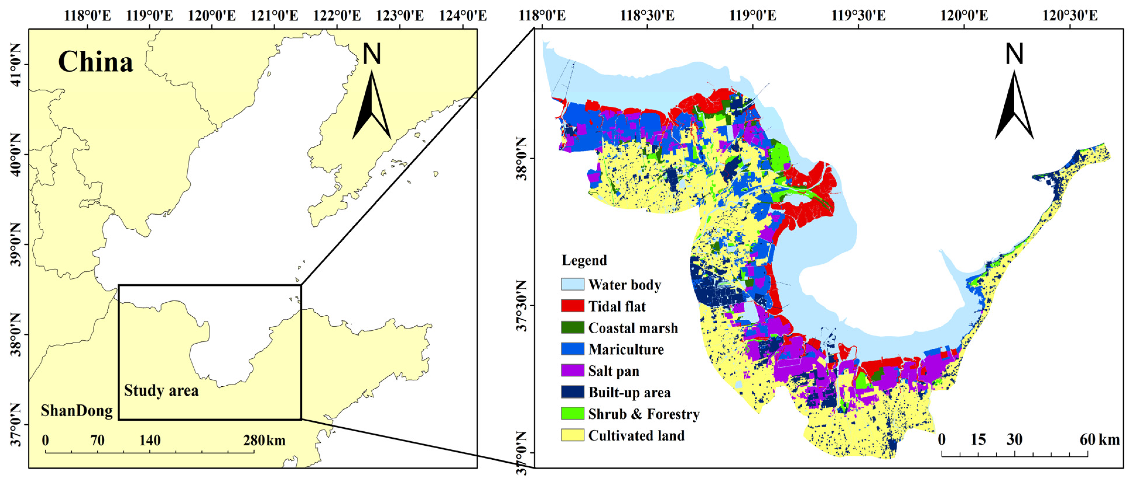
2.1. Study Area

The Yellow River Delta is located at the mouth of the Yellow River in Shandong Province, China. It spans 117°31′–120°32′E in longitude and 36°55′–38°16′N in latitude [28], with an area of 12,038 km² (Figure 1). The Yellow River Delta has a continental temperate monsoon climate with four seasons. The annual average rainfall is 530–560 mm, and the summer rainfall accounts for about 70% of the whole year [29]. The Yellow River Delta is known as the “international airport for birds”. Tens of thousands of birds roost and forage in the wetland, and it is the transit station for bird migration every year. When the upper reaches of the Yellow River flow into the sea, a large amount of sediment is deposited in the lower reaches and forms the Yellow River Delta [30], which is the second-largest estuarine delta in China and the third-largest estuarine delta in China together with the Yangtze River Delta and the Pearl River Delta. The alluvium of the Yellow River is the main part of the parent material of the Yellow River Delta, and the tidal soil and saline soil are the main soil types. The Yellow River Delta is a typical coastal wetland blue-carbon ecosystem in China that is dominated by coastal salt marsh vegetation. The main salt marsh vegetation is spartina, reed, and saltgrass [31].

2.2. Data

2.2.1. Vegetation Index Data

Leaf Area Index (LAI) data used in this study is derived from MOD15A2 (8 days, 500 m). LAI is indispensable for calculating surface photosynthesis, evapotranspiration, and net primary productivity. Normalized Difference Vegetation Index (NDVI) is derived from MOD13Q1 (16 days, 250 m) and MYD13Q1 (16 days, 250 m). The 8-day, 250m resolution NDVI data used were synthesized using MOD13Q1 and MYD13Q1. The pre-processing of LAI and NDVI data includes band extraction, projection transformation, region of interest extraction, and data format conversion. The LAI data and NDVI data used are from the ORNL DAAC (http://daac.ornl.gov, accessed on 18 March 2022).

2.2.2. Meteorological Data

The meteorological data used are wind speed, saturated water vapor pressure difference, average daily temperature, precipitation, and total radiation, of which the total radiation data are from the China Meteorological Data Sharing Network (http://data.cma.cn/, accessed on 24 March 2022) and the others are from the ERA-Interim atmospheric reanalysis dataset (https://cds.climate.copernicus.eu/#!/search?text=era5&keywords=((%20%22Spatial%20coverage:%20Global%22%20)), accessed on 30 March 2022).

2.2.3. LULC Data

LULC data were obtained from the Northeast Institute of Geography and Agroecology, Chinese Academy of Sciences. The maps in raster format are visually interpreted from remote sensing data downloaded from the United States Geological Survey Data Center (http://glovis.usgs.gov/, accessed on 7 April 2022), where LULCs are categorized into eight main types (

Table 1. LULC types.

Code	1	2	3	4	5	6	7	8
LULC types	Water body	Tidal flat	Coastal marsh	Mariculture	Salt pan	Built-up area	Shrub & Forest	Cultivated land

).

2.2.4. Observation Data

Using the net primary productivity data product of 2000 on the website of the Resources and Environmental Sciences and Data Center of the Chinese Academy of Sciences (RDCAS) (https://www.resdc.cn, accessed on 18 April 2022), AGB data of the Yellow River Delta in 2000 was obtained by using the carbon conversion coefficient of 0.475 in order to verify the simulated results in this study [32].

2.3. Method

2.3.1. Overview of BEPS

The Boreal Ecosystem Productivity Simulator (BEPS) is a remote sensing mechanism model developed from the Forest-BGC (Forest Biogeochemical Cycles) model [33]. The model combines hydrology, plant physiology, ecology, meteorology, and biophysics to simulate plant respiration, photosynthesis, carbon allocation, energy balance, and water balance [34]. The model consists of four parts: the physiological regulation model, the carbon cycle model, the water cycle model, and the energy transport model [35]. It was mainly used to simulate the productivity of the boreal forest ecosystem in Canada at first, and then gradually used to simulate the productivity of the terrestrial ecosystem in parts of China and East Asia [36]. Leaf-scale physiological and ecological models are the basis of the BEPS model [35]. The characteristics of this study are that leaves are divided into positive leaves (sunlight leaves) and negative leaves (shaded leaves). The positive leaves mainly receive direct solar radiation, while the negative leaves mainly receive scattered radiation. The leaves were divided into sunlight and shaded leaves in order to better simulate the diurnal variation of canopy photosynthesis [37]. The BEPS model is capable of simulating net primary productivity, gross primary productivity, evapotranspiration, and AGB [38,39,40]. In this study, the BEPS model simulates the dynamic process of AGB in ecosystems on a yearly scale. The spatial resolution of the BEPS model depends on the spatial resolution of the input data. The spatial resolution of the AGB simulation results in this study is 500 m. In this study, the BEPS model was run in Pycharm software. The core formulation of the BEPS model is as follows [37]:

$$AGB=NPP\times \mathrm{C}$$

(1)

where NPP stands for net primary productivity and C stands for carbon conversion factor.

$$NPP=GPP-R_a$$

(2)

where GPP represents gross primary productivity and R_a represents plant autotrophic respiration.

$$R_a=R_m+R_g$$

(3)

where R_m represents vegetation maintenance respiration and R_g stands for vegetation growth respiration.

$$GPP=A_{canopy}\times {Factor}_{GPP}\times daylength$$

(4)

where A_canopy is canopy photosynthetic rate, unit conversion factor Factor_GPP is from umol m⁻² s⁻² to g C m⁻² day⁻¹, and daylength is the length of a day.

$$A_{canopy}=A_{sun}{LAI}_{sun}+A_{shade}{LAI}_{shade}$$

(5)

where A_sun is the photosynthetic rate of positive leaves and A_shade is the photosynthetic rate of negative leaves. LAI_sun and LAI_shade are the leaf area indices of the positive and negative leaves, respectively.

2.3.2. Mapping the Driving Processes

The driving processes is represented by the initial state and final state of LULC, which is used to analyze the relationship between AGB and anthropogenic and natural driving processes. Driving processes refer to the factors that determine the transformation process of LULC (

Table 2. The driving process is represented by the initial and final states of the Yellow River Delta LULC. Abbreviations for driving processes are in brackets.

Driving Process	Accretion (A)	Restoration (Re)	Succession (S)	Reclamation (Rc)	Erosion (E)	Regressive Succession (Rs)	Replace (Rp)
Initial-final LULC types	1–2, 1–3, 1–7	(4, 5, 6, 8)-1, (4, 5, 6, 8)-2, (4, 5, 6, 8)-3, (4, 5, 6, 8)-7	2–3, 2–7, 3–7	(1, 2, 3, 7)-4, (1, 2, 3, 7)-5, (1, 2, 3, 7)-6, (1, 2, 3, 7)-8	2–1, 3–1, 7–1	3–2	(4, 5, 6)-8, (4, 5, 8)-6, (4, 6, 8)-5, (5, 6, 8)-4

). These factors can be divided into human and natural factors, respectively defined as Accretion, Restoration, Succession, Reclamation, Erosion, Regressive succession, and Replace, and each different driving process is associated with one or more corresponding initial-final LULC types [41,42]. Compared with the succession (A, S, E, Rs) dominated by natural factors, there are more LULC transformation types under the succession (Re, Rc, Rp) dominated by human intervention, in which the driving processes Re and Rc have an opposite relationship in the beginning and end states of LULC. From mariculture, salt span, built-up area, and cultivable land to water bodies, tidal flats, coastal marshes, and forestry and shrubs, it is the driving process Re; otherwise, it is the driving process Rc. The corresponding relationship between number and LULC type in Table 2 is described in Table 1.

2.3.3. Indicators of Evaluation

In this study, R²_score (R²) was used to evaluate the simulation effect of the model, and Pearson coefficient (r) was used to describe the correlation between the simulation results and the verification data more accurately.

$$\mathrm{The}{\mathrm{R}}^2=1-\frac{{\sum }_{\mathrm{i}}{({\mathrm{y}}_{\mathrm{i}}-{\mathrm{x}}_{\mathrm{i}})}^2}{{\sum }_{\mathrm{i}}{(\stackrel{\mathrm{-}}{\mathrm{x}}-{\mathrm{x}}_{\mathrm{i}})}^2}$$

(6)

$$\mathrm{The}\mathrm{r}=\frac{{\sum }_i(x_i-\overline{x})(y_i-\overline{y})}{\sqrt{{\sum }_i{(x_i-\overline{x})}^2}\sqrt{{\sum }_i{(y_i-\overline{y})}^2}}$$

(7)

In Formulas (1) and (2), x_i represents the value of the i^th verification data, $\overline{x}$ represents the average value of the verification data, y_i represents the value of the i^th simulation result, and $\overline{y}$ represents the average value of the simulation result. When R² = 1, it indicates that the simulation results are exactly equal to the validation data. The closer R² is to 1, the closer the simulation results are to the validation data. The value of the Pearson correlation coefficient ranges from −1 to 1. The larger the absolute value, the stronger the correlation. When the value is greater than 0, a positive correlation exists between the simulation results and the validation data.

2.3.4. Spatiotemporal Dynamic Analysis

In this study, different LULC types are represented by different numbers (Table 1). First, the LULC transition matrix from 2000 to 2015 was made using the raster calculator in arcgis software. The calculation principle is as follows: the number corresponding to the LULC type in 2000 is multiplied by 100, the number corresponding to the LULC type in 2010 is multiplied by 10, and the number corresponding to the LULC type in 2015 is added together.

To analyze the time dynamic change of AGB under the influence of the driving process, this study adopts the method of a heat map to present it more intuitively. The AGB dynamic heat map from 2000 to 2015 was produced using origin software. The AGB values for each specific driving process in 2000, 2010, and 2015 were normalized using Z-integrals. The expression of the Z integral is (x − u)/σ, where x is the AGB value, u is the mean value of the AGB value under a specific driving process, and σ is the standard deviation of the AGB value.

In order to analyze the spatial dynamics of AGB under the influence of the driving process, the numerical changes of AGB from 2000 to 2015 were divided into four categories in combination with the LULC driving process. The spatial regions where AGB increases or decreases under the influence of multiple driving processes are denoted by types Multi+ and Multi-, respectively, and those where AGB increases or decreases under the influence of one driving process are denoted by types Mono+ or Mono-, respectively.

3. Results and Discussion

3.1. Change Results and Evolutionary Processes of LULC during 2000–2015

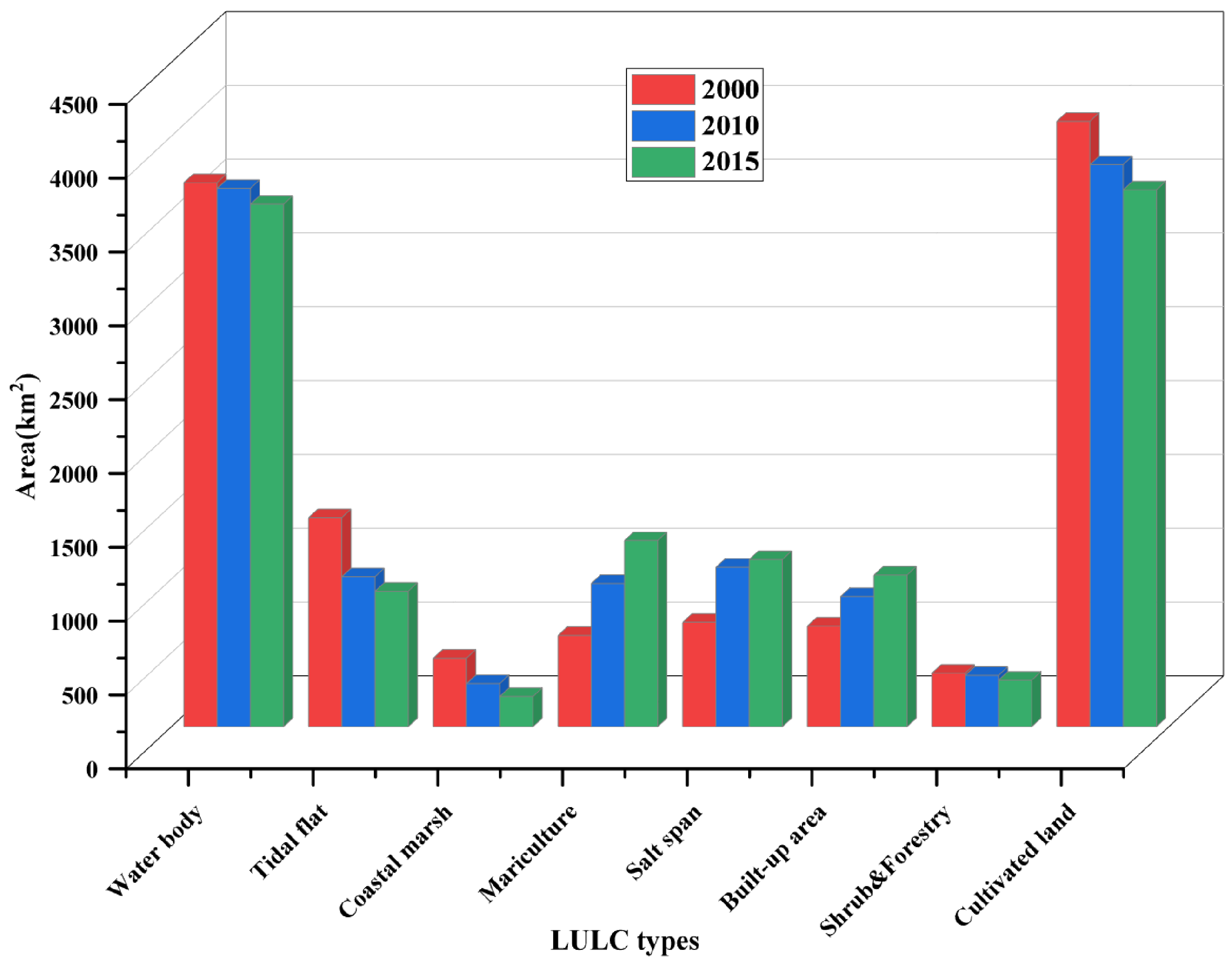
3.1.1. Changes in LULC in Study Area

Figure 2 shows that between 2000 and 2010, the LULC types that increased in the area included mariculture, salt span, and built-up area, while the LULC types that decreased in the area included water bodies, tidal flats, coastal marshes, shrub and forestry, and cultivated land. The area increased the most in salt span and the least in a built-up area. The largest reduction in area was in tidal flats, and the smallest was in shrubs and forestry. The types of LULC that increased or decreased in the area between 2010 and 2015 were the same as those between 2000 and 2010. The largest increase in area was in mariculture, and the smallest increase in area was in salt production. The largest decrease in the area was in cultivated land, and the smallest decrease in the area was in shrub and forestry. Water bodies and cultivated land were the two LULC types with the largest areas from 2000 to 2015, and the area of both has been decreasing. The tidal flat has been decreasing in size, losing 400 km² between 2000 and 2010 and 98 km² between 2010 and 2015. The area of the slat span has been increasing, with a 52.8% increase in area from 2000 to 2010 and a relatively small increase of 4.8% from 2010 to 2015. Coastal marsh and shrub and forest have been the two types of LULCs with the least area from 2000 to 2015, and their area shows a decreasing trend. In 2000, 2010, and 2015, the area values for all LULC types were concentrated in three ranges. Coastal marsh, shrub, and forest areas did not have area values of more than 470 km² and were concentrated between 200 and 470 km². Tidal flats, mariculture, salt span, and build-up areas have area values concentrated between 610 and 1420 km². The area value of water bodies and cultivated land is not less than 3530 km², concentrated between 3530 and 4110 km², which is more than seven times the respective area of coastal marsh, shrubland, and forestry.

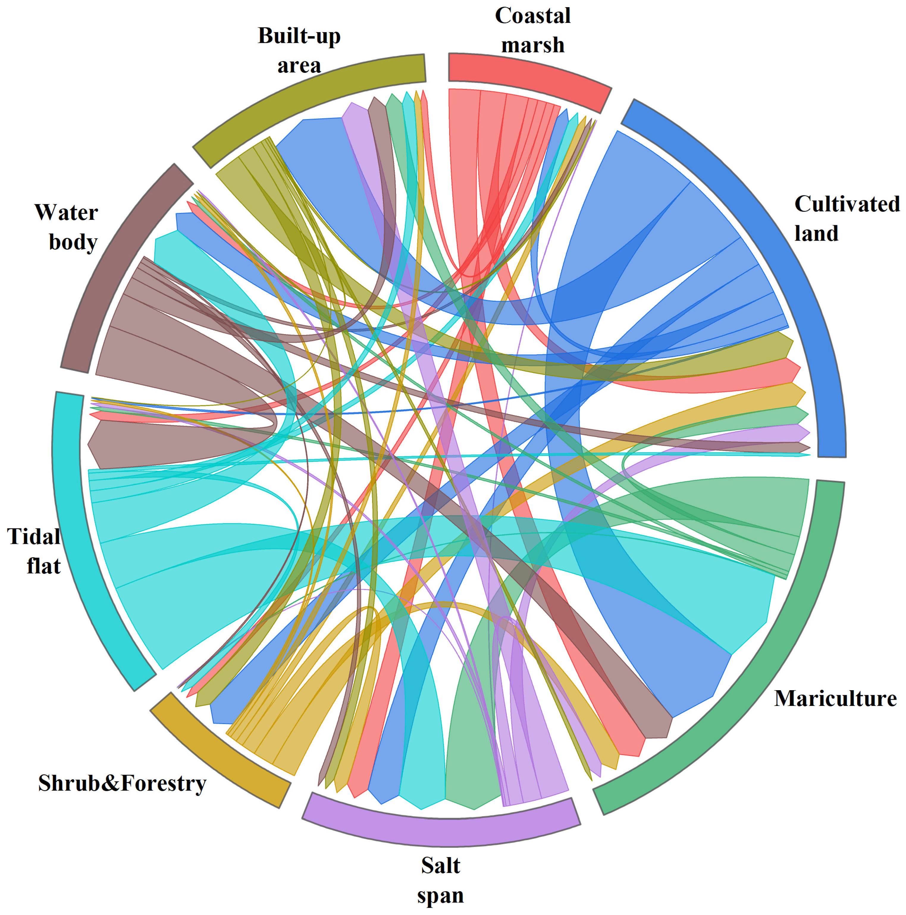
3.1.2. Cumulative Transformation between LULC Types

Figure 3 shows that from 2000 to 2015, a total of 55 LULC conversion types occurred, with a total area of 6628 km². Among them, tidal flats, mariculture, salt spans, and cultivated land of natural LULC play important import and export roles in the transformation process of LULC. During the transformation of LULC, the area gained by tidal flat restoration (253 km²) was far less than the area lost by reclamation (750 km²). Therefore, the tidal flat has the largest net area loss during the transformation of LULC, and the main LULC types lost to conversion are mariculture, salt span, and water body. During the conversion of LULC, the area gained by converting other LULC types to mariculture (1002 km²) is much larger than the area reduced by reverting to other LULC types (358 km²). Therefore, the largest net increase in area is achieved during LULC conversion. The main types of LULC converted to mariculture are coastal marsh, cultivated land, tidal flats, and water bodies. The area of salt span increased by 429 km². The LULC types converted to salt span were mainly cultivated land, mariculture, and tidal flat. The area of cultivated land decreased by 468 km², and the net area loss was second only to tidal flats. The main LULC types converted were built-up areas and mariculture. The area of shrubs and forest basically maintained balance. The area of buildup increased by 343 km². Cultivated land was the main type of LULC converted to a build-up area, and 259 km² of cultivated land were converted ta o build-up area. The area of coastal marsh was reduced by 258 km². The main LULC types were mariculture and cultivated land. The area of the water body was reduced. The main LULC types converted are mariculture and tidal flat. It can be seen in the statistical table of the LULC type conversion percentage of the Yellow River Delta in 2015 compared with 2000 (

Table 3. Statistical Table of LULC type conversion percentage in the Yellow River Delta from 2000 to 2015 (%).

	2015	Built-Up Area	Coastal Marsh	Cultivated Land	Mariculture	Salt Span	Shrub& Forestry	Tidal Flat	Water Body	Type Conversion
2000
Built-up area		66.52	1.32	14.54	2.35	4.85	8.96	0.15	1.32	33.48
Coastal marsh		4.97	15.12	19.65	23.76	16.63	6.05	7.13	6.7	84.88
Cultivated land		6.32	1.07	77.44	7.56	2.76	2.66	0.17	2.02	22.56
Mariculture		9.89	0	10.53	41.98	32.74	0.32	2.27	2.27	58.02
Salt span		13.92	0.28	9.23	6.68	66.76	0.14	1.99	0.99	33.24
Shrub& Forestry		6.63	7.18	23.76	20.17	13.81	22.65	2.21	3.59	77.35
Tidal flat		2.97	2.54	0.85	22.97	11.73	1.84	47	10.11	53
Water body		1.74	0.49	1.06	3.28	0.6	0.16	4.78	87.9	12.1

). There is a dramatic transition between natural (coastal marsh, shrub and forest, tidal flat, water body) and constructed (built-up area, cultivated land, mariculture, salt span) wetlands. 65.01% of coastal marsh, 64.37% of shrub and forestry, 38.52% of tidal flats, and 6.68% of water bodies were converted to constructed wetlands. 11.75% of the build-up area, 5.92% of cultivated land, 4.86% of mariculture, and 3.4% of salt span were converted to natural wetlands.

3.2. AGB Simulation Results Validation and Change Analysis

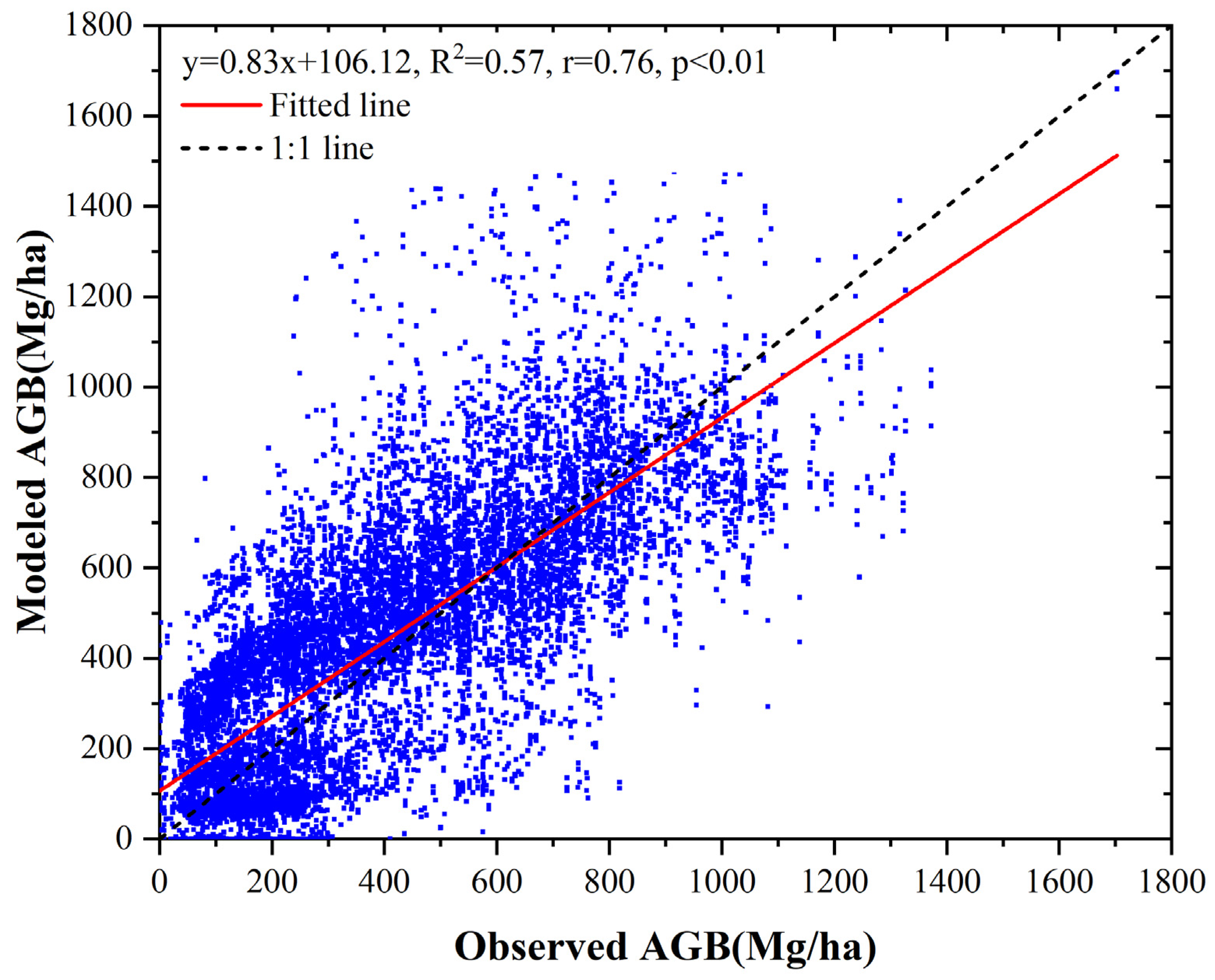
3.2.1. Validation of the AGB Calculation

This study adopted two ways to validate the simulation results. First, the AGB data of the Yellow River Delta was converted from the 2000 net primary productivity data product on the RDCAS and compared with the simulated data in this study (Figure 4). The comparative results showed the correlation was positive (r = 0.76), and the simulated value was very close to the validation value (R² = 0.57). The slope and intercept of the simulated line equation for the linear relationship between the verified data value and the simulated value are 0.83 and 106.12, respectively, and the simulated line is very close to the 1:1 line. These indicate that the BEPS model has better simulation results.

The second method of verification is to compare the results of previous studies. The range of AGB simulation results in this study (0–27 Mg/ha) is roughly the same as that of Chen et al. (0–55 Mg/ha) [31] and Han et al. (0–27 Mg/ha) [43]. Although the simulated value range of Chen et al. is much larger, the area of the simulated value of AGB beyond 27 Mg/ha is very small. They are using the regression method of machine learning. The reason for the difference in the range of simulation values between the previous study and the present study may be caused by the differences in the study period and the adopted model. In this study, the AGB in 2000, 2010, and 2015 were simulated. The research period of Chen et al. was 2019, and the research period of Han et al. was 2014.

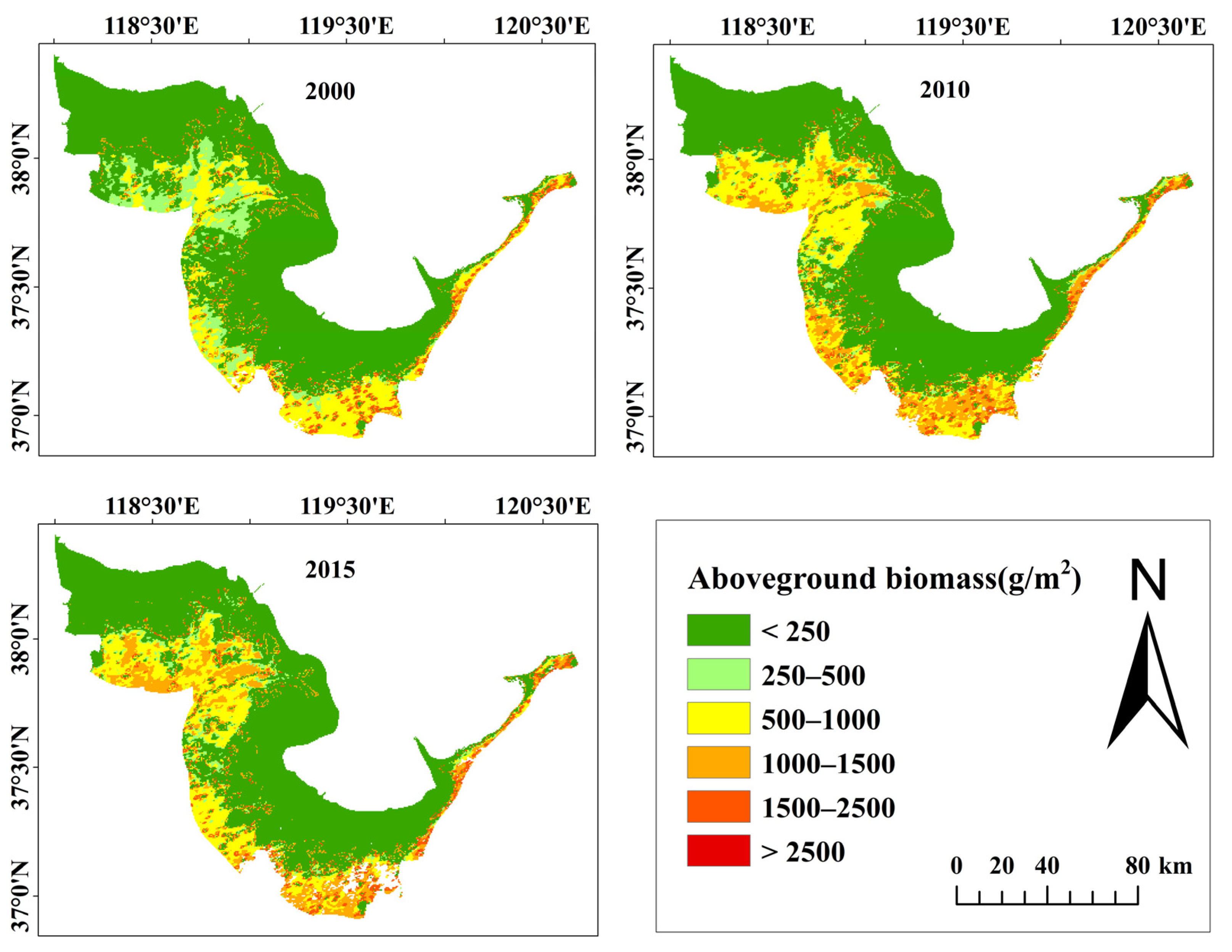
3.2.2. AGB Change under the Influence of the Driving Process

Figure 5 shows that from 2000 to 2015, coastal AGB stocks remained stable within the tidal saltwater region and have been changing in the inland land region and elsewhere. A total of 28 LULC driving processes affected AGB. From 2000 to 2010, AGB showed an increasing trend, with an increase of 407,770 Mg. From 2010 to 2015, it showed a decreasing trend, with a decrease of 21,649 Mg. The 26 main LULC driving processes affected 99.9% of the LULC conversion area, accounting for 32.8% of the total area of the Yellow River Delta. The AGB of the corresponding LULC conversion area in the Yellow River Delta increased by 386,121 Mg.

3.3. Analysis of the Influence Process of LULC Changes on AGB

3.3.1. The Total Change in AGB Associated with the Driving Processes

Figure 6 shows that during the period 2000–2015, of the 26 main LULC driving processes, 22 were accompanied by an increase in AGB, and four were accompanied by a decrease in AGB, which were 390,111 Mg and 5024 Mg respectively (Figure 6). There are seven driving processes accompanied by the largest amount of change: Re-Rc, Rc-Rp, Rc, Re, S-Rc, Rc-Re, and Rp. At the same time, the AGB value of these seven driving processes increases, among which the AGB value of Re-Rc and Rc-Re has seen a significant change in the past 15 years. Under the driving process of Re-Rc, AGB was in a state of growth from 2000 to 2010 and a state of decline from 2010 to 2015. Under the driving process Rc-Re, AGB has been in a state of growth from 2000 to 2015, while the AGB values of the other five driving processes are relatively flat.

Among the four driving processes of AGB reduction, the net change in the past 15 years has been quite different. The largest reduction is E, which is much larger than E-Rc, Rs-E, and Rs-Rc, and the least reduction is Rs-E. The AGB value of Rs-Rc in 2010 was at a high level compared with that in 2000 and 2015. The AGB values of Rs-E, E-Rc, and E in 2000 are at a high level compared with those in 2010 and 2015. The net change in AGB under two driving processes is particularly insignificant. A-Rs and A-S, under which the AGB value was at a relatively high level in 2010. The net variation of A-Rs and A-S is 38 Mg and 149 Mg respectively, and the difference in the net variation of these two driving processes is 111 Mg, which is a large gap. The dynamic graph of AGB shows that in 2000, AGB were relatively small on the whole and then kept in a state of increase compared to 2000.

The change in AGB in the LULC conversion area under some driving processes is related to the change in vegetation type in the area. For example, the driving process Rs brought a net increase in AGB. In the LULC conversion area driven by Rs, spartina alterniflora was introduced into the intertidal zone near the Yellow River Delta in 1990 and began to spread explosively in the nature reserve in 2010. Its strong reproductive ability gradually led to the encroachment of the habitats of the local salt ground and sea grass beds and the decrease of the densities of benthic organisms in the tidal plains. The decrease or loss of birds’ foraging and habitat will do great harm to the biodiversity of nature reserves [44].

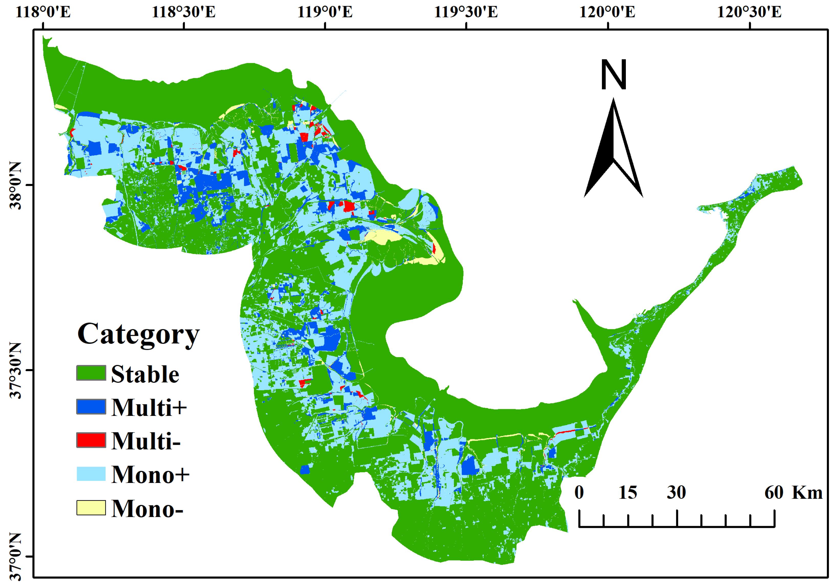
3.3.2. Change of AGB in Multiple and Single Driving Processes

There is no LULC conversion between the water body and the inland area in the Yellow River Delta, and the LULC conversion area is between the water body and the inland area (Figure 7). Only a small amount of AGB decreases in LULC transition regions. The driving processes that cause AGB reduction include three multiple driving processes and one single driving process. The reduction of single driving process E accounted for 71.5% of all reduction species, which led to the largest reduction. Multi+ types occupy 7% of the Yellow River Delta area, among which the two human-driven processes (Rc-Rp and Re-Rc) contribute the most. The growth of Multi+ types accounted for 27.4% of all the growth, and the total growth of the driving processes Rc-Rp and Re-Rc accounted for 15.3% of all the growth. Mono+ types occupy 23.9% of the area of the Yellow River Delta, in which human-driven processes (Rp) contribute more, and Mono+ increases account for 72.6% of all increases.

3.3.3. Changes in AGB under Human-Induced, Natural, and Human-Natural Coupling Driving Processes

The changes in AGB under the driving process are analyzed from the perspectives of human-induced, natural, and human-natural coupling. Among the 26 main driving processes, there are seven human-driven processes, 11 natural-driven processes, and eight human-naturally coupled processes (

Table 4. The driving process categories of artificial, natural, and human-natural coupling contain specific driving processes respectively.

Types	Human-Induced	Natural	Human-Natural Coupling
Driving process	Rp-Re, Rc-Rp, Rc, Re Rc-Re, Rp, Re-Rc	A-Rs, Rs-S, Rs-E, A-S S-Rs, A-E, E-A, Rs, E A, S	Re-Rs, E-Rc, A-Rc, S-Rc Re-E, Rs-Rc, Re-A, Re-S

). From 2000 to 2015, human-driven processes contributed 90.7% to the increase of AGB, in which the driving process Rp contributed the most to the increase of AGB, increasing 55.3% to AGB, while the human-driven process Rp-Re contributed the least to the increase of AGB, increasing 1.4% to AGB. In addition to the AGB change under human-driven process Rp, the AGB increase brought by the other six kinds of human-driven processes accounted for 81.3% of the 25 kinds of main driving processes, excluding human-driven process Rp.

The human-natural coupling process resulted in a 5.5% AGB increase and a 23% AGB loss. Under human-natural coupling driving processes, S-Rc contributed the most to the increase in AGB, accounting for 3.4% of the total increase in AGB. The natural driving processes resulted in a 3.8% AGB increase and a 77% AGB loss. Under the natural driving process, the AGB loss is brought by Rs-E and E, in which E brings 71.5% of the loss, accounting for the largest proportion of the total AGB loss.

The gains and losses of AGB in LULC conversion zones are not equal in both man-made and natural processes. Especially under the single human-driven process Rp, among the 26 main driving processes, Rp brings the largest AGB benefit due to its huge area. Since multiple processes contain more than one human-driven or natural-driven process, it is possible to separately analyze the benefits or losses brought by human-driven or natural-driven processes in multiple processes from multiple periods. The net increase in AGB in the human-naturally coupled driving process Re-E is due to the fact that the AGB income brought by the driving process Re from 2000 to 2010 is greater than the AGB loss brought by the driving process E from 2010 to 2015. AGB can also be affected by a variety of factors. The carrier of vegetation is soil. Soil moisture content, soil organic matter, water-soluble salt, pH value, nitrogen, phosphorus, and other components of soil will affect vegetation growth and the distribution of AGB [43,45].

4. Conclusions

In this study, LULC data and the BEPS model were used to explore the relationship between LULC transformation under anthropogenic and natural driving processes and AGB dynamics in the Yellow River Delta during 2000–2015. The results showed that the BEPS model can better simulate AGB in the Yellow River Delta with R² = 0.57. And the AGB of the LULC conversion area, which accounted for 30.9% of the Yellow River Delta area, increased by a total of 391,145 Mg. The AGB of the LULC conversion area, which accounted for 1.9% of the Yellow River Delta area, decreased by a total of 5024 Mg. The conversion of coastal wetlands to built-up areas, mariculture, and salt span decreased by 755 km² from 2000 to 2015, and the AGB of the Yellow River Delta LULC conversion area increased by 386,121 Mg. In general, the changes in AGB showed an increasing trend throughout the study period. Single-drive process E resulted in a 71.5% reduction in AGB. 72.6% of the increase in AGB was related to single artificial (e.g., Restore) or natural (e.g., Accretion) driving processes, and 27.4% of the increase in AGB was related to multiple driver processes, especially those that were coupled with natural. Furthermore, naturally driven processes bring far more AGB benefits than losses, while human-driven processes bring the largest AGB benefits, especially human-driven processes’ Rp. Based on the LULC type transformation of coastal wetlands in the Yellow River Delta, this study accurately analyzed the temporal and spatial dynamic changes of AGB, which has important reference significance for planning the future LULC of wetlands and improving AGB.

References

1. Lhakpa, D.; Fan, Y.; Cai, Y. Continuous Karakoram Glacier Anomaly and Its Response to Climate Change during 2000–2021. Remote Sens. 2022, 14, 6281. [Google Scholar] [CrossRef]
2. Briere, M.D.; Gajewski, K. Holocene human-environment interactions across the Northern American prairie-forest ecotone. Anthropocene 2023, 41, 100367. [Google Scholar] [CrossRef]
3. Chemeda, B.A.; Wakjira, F.S.; Hizikias, E.B. Tree diversity and biomass carbon stock analysis along altitudinal gradients in coffee-based agroforestry system of Western Ethiopia. Cogent Food Agric. 2022, 8, 2123767. [Google Scholar] [CrossRef]
4. Sadai, S.; Spector, R.A.; DeConto, R.; Gomez, N. The Paris Agreement and Climate Justice: Inequitable Impacts of Sea Level Rise Associated With Temperature Targets. Earth’s Future 2022, 10, e2022EF002940. [Google Scholar] [CrossRef]
5. Zhao, X.; Ma, X.; Chen, B.; Shang, Y.; Song, M. Challenges toward carbon neutrality in China: Strategies and countermeasures. Resour. Conserv. Recycl. 2022, 176, 105959. [Google Scholar] [CrossRef]
6. Wang, Y.; Guo, C.-h.; Chen, X.-j.; Jia, L.-q.; Guo, X.-n.; Chen, R.-s.; Zhang, M.-s.; Chen, Z.-y.; Wang, H.-d. Carbon peak and carbon neutrality in China: Goals, implementation path and prospects. China Geol. 2021, 4, 720–746. [Google Scholar] [CrossRef]
7. Rindfuss, R.R.; Entwisle, B.; Walsh, S.J.; An, L.; Badenoch, N.; Brown, D.G.; Deadman, P.; Evans, T.P.; Fox, J.; Geoghegan, J.; et al. Land use change: Complexity and comparisons. J. Land Use Sci. 2008, 3, 1–10. [Google Scholar] [CrossRef] [Green Version]
8. Mallinis, G.; Koutsias, N.; Arianoutsou, M. Monitoring land use/land cover transformations from 1945 to 2007 in two peri-urban mountainous areas of Athens metropolitan area, Greece. Sci. Total Environ. 2014, 490, 262–278. [Google Scholar] [CrossRef]
9. Ren, G.; Zhao, Y.; Wang, J.; Wu, P.; Ma, Y. Ecological effects analysis of Spartina alterniflora invasion within Yellow River delta using long time series remote sensing imagery. Estuar. Coast. Shelf Sci. 2020, 249, 107111. [Google Scholar] [CrossRef]
10. Ouyang, Z.; Wang, X.; Miao, H. A primary study on Chinese terrestrial ecosystem services and their ecological-economic values. Acta Ecol. Sin. 1999, 19, 607–613. [Google Scholar]
11. Duarte, C.M.; Losada, I.J.; Hendriks, I.E.; Mazarrasa, I.; Mazarrasa, N.M. Correction: Corrigendum: The role of coastal plant communities for climate change mitigation and adaptation. Nat. Clim. Chang. 2016, 6, 802. [Google Scholar] [CrossRef]
12. Wang, F.; Sanders, C.J.; Santos, I.R.; Tang, J.; Schuerch, M.; Kirwan, M.L.; Kopp, R.E.; Zhu, K.; Li, X.; Yuan, J.; et al. Global blue carbon accumulation in tidal wetlands increases with climate change. Natl. Sci. Rev. 2020, 8, nwaa296. [Google Scholar] [CrossRef] [PubMed]
13. Chastain, S.G.; Kohfeld, K.E.; Pellatt, M.G.; Olid, C.; Gailis, M. Quantification of blue carbon in salt marshes of the Pacific coast of Canada. Biogeosciences 2022, 19, 5751–5777. [Google Scholar] [CrossRef]
14. Mcleod, E.; Chmura, G.L.; Bouillon, S.; Salm, R.; Björk, M.; Duarte, C.M.; Lovelock, C.E.; Schlesinger, W.H.; Silliman, B.R. A blueprint for blue carbon: Toward an improved understanding of the role of vegetated coastal habitats in sequestering CO2. Front. Ecol. Environ. 2011, 9, 552–560. [Google Scholar] [CrossRef] [Green Version]
15. Sun, S.; Wang, Y.; Song, Z.; Chen, C.; Zhang, Y.; Chen, X.; Chen, W.; Yuan, W.; Wu, X.; Ran, X.; et al. Modelling Aboveground Biomass Carbon Stock of the Bohai Rim Coastal Wetlands by Integrating Remote Sensing, Terrain, and Climate Data. Remote Sens. 2021, 13, 4321. [Google Scholar] [CrossRef]
16. Macreadie, P.I.; Nielsen, D.A.; Kelleway, J.J.; Atwood, T.B.; Seymour, J.R.; Petrou, K.; Connolly, R.M.; Thomson, A.C.; Trevathan-Tackett, S.M.; Ralph, P.J. Can we manage coastal ecosystems to sequester more blue carbon? Front. Ecol. Environ. 2017, 15, 206–213. [Google Scholar] [CrossRef] [Green Version]
17. Chu, X.; Han, G.; Xing, Q.; Xia, J.; Sun, B.; Li, X.; Yu, J.; Li, D.; Song, W. Changes in plant biomass induced by soil moisture variability drive interannual variation in the net ecosystem CO2 exchange over a reclaimed coastal wetland. Agric. For. Meteorol. 2019, 264, 138–148. [Google Scholar] [CrossRef]
18. Zekarias, T.; Govindu, V.; Kebede, Y.; Gelaw, A. Geospatial Analysis of Wetland Dynamics on Lake Abaya-Chamo, The Main Rift Valley of Ethiopia. Heliyon 2021, 7, e07943. [Google Scholar] [CrossRef]
19. Aitali, R.; Snoussi, M.; Kolker, A.S.; Oujidi, B.; Mhammdi, N. Effects of Land Use/Land Cover Changes on Carbon Storage in North African Coastal Wetlands. J. Mar. Sci. Eng. 2022, 10, 364. [Google Scholar] [CrossRef]
20. Minta, M.; Kibret, K.; Thorne, P.; Nigussie, T.; Nigatu, L. Land use and land cover dynamics in Dendi-Jeldu hilly-mountainous areas in the central Ethiopian highlands. Geoderma 2018, 314, 27–36. [Google Scholar] [CrossRef]
21. Massetti, A.; Gil, A. Mapping and assessing land cover/land use and aboveground carbon stocks rapid changes in small oceanic islands’ terrestrial ecosystems: A case study of Madeira Island, Portugal (2009–2011). Remote Sens. Environ. 2020, 239, 111625. [Google Scholar] [CrossRef]
22. Acheampong, J.O.; Attua, E.M.; Mensah, M.; Fosu-Mensah, B.Y.; Apambilla, R.A.; Doe, E.K. Livelihood, carbon and spatiotemporal land-use land-cover change in the Yenku forest reserve of Ghana, 2000–2020. Int. J. Appl. Earth Obs. Geoinf. 2022, 112, 102938. [Google Scholar] [CrossRef]
23. Li, Y.; Qiu, J.; Li, Z.; Li, Y. Assessment of Blue Carbon Storage Loss in Coastal Wetlands under Rapid Reclamation. Sustainability 2018, 10, 2818. [Google Scholar] [CrossRef] [Green Version]
24. Liu, J.; Chen, J.M.; Cihlar, J.; Park, W.M. A process-based boreal ecosystem productivity simulator using remote sensing inputs. Remote Sens. Environ. 1997, 62, 158–175. [Google Scholar] [CrossRef]
25. Liu, J.; Chen, J.M.; Cihlar, J.; Chen, W. Net primary productivity distribution in the BOREAS region from a process model using satellite and surface data. J. Geophys. Res. Atmos. 1999, 104, 27735–27754. [Google Scholar] [CrossRef]
26. Tian, H.; Liu, M.; Zhang, C.; Ren, W.; Xu, X.; Chen, G.; Lu, C.; Tao, B. The Dynamic Land Ecosystem Model (DLEM) for Simulating Terrestrial Processes and Interactions in the Context of Multifactor Global Change. Acta Geogr. Sin. 2010, 65, 1027–1047. [Google Scholar] [CrossRef]
27. Feng, X.; Liu, G.; Chen, J.M.; Chen, M.; Liu, J.; Ju, W.M.; Sun, R.; Zhou, W. Net primary productivity of China’s terrestrial ecosystems from a process model driven by remote sensing. J. Environ. Manag. 2007, 85, 563–573. [Google Scholar] [CrossRef]
28. Ma, T.; Li, X.; Bai, J.; Ding, S.; Zhou, F.; Cui, B. Four decades’ dynamics of coastal blue carbon storage driven by land use/land cover transformation under natural and anthropogenic processes in the Yellow River Delta, China. Sci. Total Environ. 2019, 655, 741–750. [Google Scholar] [CrossRef]
29. Yu, J.; Wang, Y.; Li, Y.; Dong, H.; Zhou, D.; Han, G.; Wu, H.; Wang, G.; Mao, P.; Gao, Y. Soil organic carbon storage changes in coastal wetlands of the modern Yellow River Delta from 2000 to 2009. Biogeosciences 2012, 9, 2325–2331. [Google Scholar] [CrossRef] [Green Version]
30. Zhao, H.; Lin, Y.; Delang, C.O.; Ma, Y.; Zhou, J.; He, H. Contribution of soil erosion to the evolution of the plateau-plain-delta system in the Yellow River basin over the past 10,000 years. Palaeogeogr. Palaeoclimatol. Palaeoecol. 2022, 601, 111133. [Google Scholar] [CrossRef]
31. Chen, C.; Ma, Y.; Ren, G.; Wang, J. Aboveground biomass of salt-marsh vegetation in coastal wetlands: Sample expansion of in situ hyperspectral and Sentinel-2 data using a generative adversarial network. Remote Sens. Environ. 2022, 270, 112885. [Google Scholar] [CrossRef]
32. Raich, J.W.; Rastetter, E.B.; Melillo, J.M.; Kicklighter, D.W.; Steudler, P.A.; Peterson, B.J.; Grace, A.L.; Moore, B., III; Vorosmarty, C.J. Potential Net Primary Productivity in South America: Application of a Global Model. Ecol. Appl. 1991, 1, 399–429. [Google Scholar] [CrossRef] [Green Version]
33. Running, S.W.; Coughlan, J.C. A general model of forest ecosystem processes for regional applications I. Hydrologic balance, canopy gas exchange and primary production processes. Ecol. Model. 1988, 42, 125–154. [Google Scholar] [CrossRef]
34. Farquhar, G.D.; von Caemmerer, S.; Berry, J.A. A biochemical model of photosynthetic CO2 assimilation in leaves of C3 species. Planta 1980, 149, 78–90. [Google Scholar] [CrossRef] [Green Version]
35. Qiang, Y.; Wang, T.-D. Simulation of the Physiological Responses of C3 Plant Leaves to Environmental Factors by a Model Which Combines Stomatal Conductance, Photosynthesis and Transpiration. J. Integr. Plant Biol. 1998, 40, 740–750. [Google Scholar]
36. Nanzad, L.; Zhang, J.; Tuvdendorj, B.; Yang, S.; Rinzin, S.; Prodhan, F.A.; Sharma, T.P.P. Assessment of Drought Impact on Net Primary Productivity in the Terrestrial Ecosystems of Mongolia from 2003 to 2018. Remote Sens. 2021, 13, 2522. [Google Scholar] [CrossRef]
37. Chen, J.M.; Liu, J.; Cihlar, J.; Goulden, M.L. Daily canopy photosynthesis model through temporal and spatial scaling for remote sensing applications. Ecol. Model. 1999, 124, 99–119. [Google Scholar] [CrossRef] [Green Version]
38. Zhang, S.; Zhang, J.; Bai, Y.; Koju, U.A.; Igbawua, T.; Chang, Q.; Zhang, D.; Yao, F. Evaluation and improvement of the daily boreal ecosystem productivity simulator in simulating gross primary productivity at 41 flux sites across Europe. Ecol. Model. 2018, 368, 205–232. [Google Scholar] [CrossRef]
39. Liu, J.; Chen, J.M.; Cihlar, J. Mapping evapotranspiration based on remote sensing: An application to Canada’s landmass. Water Resour. Res. 2003, 39, 1189. [Google Scholar] [CrossRef]
40. Liu, J.; Chen, J.M.; Cihlar, J.; Chen, W. Net primary productivity mapped for Canada at 1-km resolution. Glob. Ecol. Biogeogr. 2002, 11, 115–129. [Google Scholar] [CrossRef] [Green Version]
41. Kim, W. Flood-built land. Nat. Geosci. 2012, 5, 521–522. [Google Scholar] [CrossRef]
42. Kirwan, M.L.; Megonigal, J.P. Tidal wetland stability in the face of human impacts and sea-level rise. Nature 2013, 504, 53–60. [Google Scholar] [CrossRef] [PubMed]
43. Han, M.; Pan, B.; Liu, Y.B.; Yu, H.Z.; Liu, Y.R. Wetland biomass inversion and space differentiation: A case study of the Yellow River Delta Nature Reserve. PLoS ONE 2019, 14, e0210774. [Google Scholar] [CrossRef] [Green Version]
44. Chen, M.; Ke, Y.; Bai, J.; Li, P.; Lyu, M.; Gong, Z.; Zhou, D. Monitoring early stage invasion of exotic Spartina alterniflora using deep-learning super-resolution techniques based on multisource high-resolution satellite imagery: A case study in the Yellow River Delta, China. Int. J. Appl. Earth Obs. Geoinf. 2020, 92, 102180. [Google Scholar] [CrossRef]
45. Liu, L.; Han, M.; Liu, Y.B.; Pan, B. Spatial distribution of wetland vegetation biomass and its influencing factors in the Yellow River Delta nature reserve. Shengtai Xuebao/Acta Ecol. Sin. 2017, 37, 4346–4355. [Google Scholar]
Figure 1. Location map of the study area and LULC in the Yellow River Delta in 2015.
Remotesensing 15 03966 g001
Figure 2. Area changes of eight LULC types in the Yellow River Delta from 2000 to 2015.
Remotesensing 15 03966 g002
Figure 3. Cumulative area of conversion between eight LULC types in the Yellow River Delta from 2000 to 2015. The eight colors represent the eight LULC types, forming a circle. Each ribbon within the circle points from the original LULC type (start of the arc) to the final LULC type (sharp corner end).
Remotesensing 15 03966 g003
Figure 4. Validation of the simulated AGB with observed data in the Yellow River Delta.
Remotesensing 15 03966 g004
Figure 5. AGB distribution map of the Yellow River Delta from 2000 to 2015.
Remotesensing 15 03966 g005
Figure 6. AGB dynamics under the influence of the main driving process. The color intensity of each rectangle in the figure represents the standardized AGB under a specific driving process, and the color change under a specific driving process represents the change in the value of AGB under this driving process from 2000 to 2015. Total is the net change in AGB from 2000 to 2015, and the unit is Mg. Connect multiple driving processes with “-” in chronological order. A: Accretion, Re: Restoration, S: Succession, Rc: Reclamation, E: Erosion, Rs: Regressive succession, Rp: Replace. Category refers to 4 AGB dynamics related to the driving process.
Remotesensing 15 03966 g006
Figure 7. Spatially, four types of AGB dynamics related to driving processes are divided to illustrate the changes in AGB under different types of driving processes. Type Mono+ and type Mono- represent increased or decreased AGB under a single driving process, and type Multi- and type Multi+ represent decreased or increased AGB under multiple driving processes. Stable Indicates the area in which the LULC does not change.
Remotesensing 15 03966 g007