Abstract
Object classification in hyperspectral images involves accurately categorizing objects based on their spectral characteristics. However, the high dimensionality of hyperspectral data and class imbalance pose significant challenges to object classification performance. To address these challenges, we propose a framework that incorporates dimensionality reduction and re-sampling as preprocessing steps for a deep learning model. Our framework employs a novel subgroup-based dimensionality reduction technique to extract and select the most informative features with minimal redundancy. Additionally, the data are resampled to achieve class balance across all categories. The reduced and balanced data are then processed through a hybrid CNN model, which combines a 3D learning block and a 2D learning block to extract spectral–spatial features and achieve satisfactory classification accuracy. By adopting this hybrid approach, we simplify the model while improving performance in the presence of noise and limited sample size. We evaluated our proposed model on the Salinas scene, Pavia University, and Kennedy Space Center benchmark hyperspectral datasets, comparing it to state-of-the-art methods. Our object classification technique achieves highly promising results, with overall accuracies of 99.98%, 99.94%, and 99.46% on the three datasets, respectively. This proposed approach offers a compelling solution to overcome the challenges of high dimensionality and class imbalance in hyperspectral object classification.
1. Introduction
A Hyperspectral Image (HSI) is a type of image that captures spectral data across hundreds of contiguous narrow wavelength bands [1] as well as spatial information about the objects in a scene. This provides a rich and detailed representation of the objects in a scene, capturing information about the color and intensity of light as well as the spectral features of the objects [2]. As a result, HSIs provide a unique combination of spectral and spatial information, making them useful for a variety of applications, including mineral and crop mapping, environmental monitoring, and military reconnaissance [3,4]. An HSI often has a large number of spectral bands, resulting in numerous features in the data. As such, the challenge of high dimensionality is a major issue in the field of HSI. The difficulty of interpreting HSIs with a large number of dimensions (or spectral bands) is often referred to as the ”curse of dimensionality” [5]. High dimensionality makes data processing and analysis difficult, increases the danger of overfitting, makes visualization difficult, and limits statistical methods. The high dimensionality of HSI demands more computational power, making it harder to process and analyze the data efficiently. To address these challenges, it is important to choose appropriate techniques and approaches for processing and analyzing HSI and to ensure that the models used can handle the high dimensionality effectively [6].
The problems around high dimensionality in object recognition from HSIs is currently addressed through classic dimensionality reduction approaches such as feature extraction and feature selection [7,8] methods. Feature extraction approaches, such as Principal Component Analysis (PCA) [9], Minimum Noise Fraction (MNF) [10], Segmented PCA [11], Segmented MNF [12], and Non-Negative Matrix Factorization (NMF) [13], aim to identify a compact set of features that represent the most important information in the data. Feature selection approaches, such as correlation-based and mutual information-based methods, focus on identifying the most relevant features and eliminating the less important ones. However, deep learning techniques, such as Convolutional Neural Networks (CNNs) [14] and Deep Belief Networks (DBNs) [15], are promisingly being applied to handle the high dimensionality problems in HSI. The best approach for a specific application depends on its needs and requirements; by carefully considering the techniques used to process and analyze the data, high dimensionality problems in HSI can be effectively addressed. Although PCA is a popular dimensionality reduction technique that is used in many fields, including hyperspectral imaging, it can have limitations in the context of HSIs due to the unique characteristics of HSI data [16]. One of the main problems with using PCA for dimensionality reduction in HSIs is that it is a linear technique that assumes a linear relationship between the features in the data [17]. However, the spectral signatures of materials in a scene can be nonlinear, which can result in PCA losing important information during the dimensionality reduction process. Another problem with PCA for HSI is that it may not preserve the spatial information in the data. This can be a critical issue in HSI, where spatial information can be used to identify the location and distribution of materials in a scene. Segmented PCA provides a superior solution over standard PCA for dimensionality reduction in hyperspectral imaging [18]. This is because it divides the data into distinct segments and processes each segment individually, enabling more effective and efficient reduction of the data’s dimensionality while preserving important spectral and spatial information. On the other hand, the standard PCA approach processes the entire dataset as one entity, which may not be suitable for handling complex relationships between features. In addition to issues with its effectiveness, standard PCA in HSI can encounter problems with preserving spectral and spatial information, as it is sensitive to noise and outliers, and is limited to linear relationships between features. The advantage of using Segmented PCA in HSI is that it enables more efficient and effective reduction of data dimensionality while retaining important spectral and spatial information through the division and individual processing of data segments.
MNF is another method for dimensionality reduction in HSI that aims to preserve the most important information in the data while reducing the dimensionality [19]. The drawback of MNF in HSI is that it can lead to the loss of important spectral information if the noise fraction is not accurately estimated, and it can be sensitive to outliers in the data. Based on the concept of segmentation, several methods have been proposed to eliminate the constraints of MNF, such as Segmented MNF and Band grouping MNF (Bg-MNF). The main difference between regular MNF and segmented MNF is that the latter involves dividing the data into segments or regions before applying the MNF transformation. The idea behind this approach is to preserve the unique spectral information in each segment and to reduce the dimensionality of the data in a more effective and efficient way. Bg-MNF is an extension of the MNF technique which is widely used for spectral data compression and feature extraction. Bg-MNF is designed to improve the performance of MNF in the presence of high levels of noise. It does this by grouping the data into smaller sub-bands, or segments, before applying the MNF transformation. This allows the algorithm to identify and suppress the background noise in each sub-band more effectively. The main advantage of Bg-MNF over standard MNF is that it can provide a more robust and stable representation of the objects in the scene even in the presence of high levels of noise. This makes Bg-MNF a useful tool for various applications, including target detection, material classification, and environmental monitoring. By reducing the dimensionality of the data while preserving important information, Bg-MNF can improve the efficiency and accuracy of these applications. Determining the optimal number and size of the sub-bands or segments in band grouping MNF can be challenging. If the sub-bands are too large, the method may not be effective in suppressing the background noise, while if they are too small the method may become computationally impractical.
NMF is a linear algebraic technique that factorizes a non-negative matrix into two non-negative matrices to extract spectral features and reduce dimensionality in hyperspectral imaging [20]. NMF is often considered to be a better alternative to both MNF and PCA for HSI analysis, as it imposes a non-negativity constraint on the factorized matrices, which helps to preserve important spectral information and reduce the impact of noise in the data while producing factors that are non-negative and have a physical meaning. This makes NMF a more interpretable [21] and robust solution compared to PCA while providing a more computationally efficient solution compared to MNF. The main problem with standard NMF for HSI analysis is that it may not be able to effectively capture and separate the different materials in a scene, leading to spectral mixing and loss of information. Segmented NMF can address this issue by dividing the hyperspectral data into segments or clusters before applying the NMF factorization, which helps to reduce the dimensionality and improve the accuracy of the resulting factors. However, spectral redundancy may persist in the data. In light of the issue, we suggest a method for subgrouping using a correlation matrix that shifts from one set of frequencies to another; this method is termed subgrouping-based NMF. The correlation matrix image is utilized in order to partition the image into smaller groupings. Therefore, SNMF uses NMF to pull out features from each group while keeping the amount of computing needed to a minimum. Classification rankings are determined using a feature selection technique that uses correlation coefficient matrices to prioritize informative feature traits while reducing irrelevant features (mRMR). After the dimensionality of the HSI has been reduced, the next step is to recognize or classify each pixel in the image.
There are several commonly used classification methods for HSIs, including Support Vector Machine (SVMs) [22], Artificial Neural Networks (ANNs) [23], Random Forest (RF) [24], and Convolutional Neural Networks (CNNs) [25]. Deep learning algorithms are often considered more suitable for HSI classification than machine learning algorithms because they can handle both spectral and spatial variability in hyperspectral data through multiple layers of nonlinear transformations. Deep learning models, especially CNNs, have become increasingly popular in the field of object classification for hyperspectral imagery because they are capable of processing high-dimensional data and extracting hierarchical features from it. Unlike machine learning models such SVM or RF, which can struggle with high-dimensional data and require separate feature extraction and classification steps, CNNs are end-to-end learning models that can learn both the feature extraction and classification tasks simultaneously [26]. Hence, state-of-the-art algorithms such as 2D CNN, 3D CNN [27], fast and compact 3D CNN [28], and HybridSN [29] have shown great promise in achieving high accuracy and robustness in HSI classification; 2D CNNs are limited to spatial information, and may not be able to capture the spectral information that is crucial for accurate classification, while 3D CNNs can leverage both spectral and spatial information, although they have higher computational cost due to the need for 3D convolutions. Fast and compact 3D CNNs aim to reduce the computational cost of 3D CNNs while maintaining high accuracy; however, they may still be too computationally expensive for resource-constrained applications. HybridSN combines both spectral and spatial information for HSI classification, although its reliance on the assumption that the spectral and spatial features can be effectively separated may not hold in all cases. This issue can be potentially addressed through the use of optimization techniques. From the above discussion, it is evident that by integrating dimensionality reduction techniques as a preprocessing step, deep learning models can effectively target the most informative features of the data, leading to superior classification performance with enhanced efficiency and accuracy. Even though effective methods have been employed for dimensionality reduction and constructive classification for HSI, the class imbalance problem persists. This problem is often overlooked in HSI object classification due to its complexity; however, it is crucial to address this issue, as it can greatly affect the accuracy of a classification model.
On the other hand, data imbalances can be easily found in HSI object recognition tasks. Imbalance occurs when one class in the data has significantly more samples than the other class, leading to a bias towards the majority class. This can result in poor performance, low sensitivity, and increased false positives for the minority class while insufficiently representing majorities in the training data [30,31]. Several solutions have been proposed to address this issue, including re-sampling techniques, cost-sensitive learning, and class weighting [32]. In statistical analysis, re-sampling techniques are frequently employed to test hypotheses and evaluate model performance by balancing the class distribution. Oversampling the minority class or undersampling the majority class are among the common methods of achieving balance [33]. Undersampling is a type of re-sampling technique that involves reducing the size of the majority class by removing samples from it. This is done in order to balance the class distribution and make the minority class more prominent in the dataset. Oversampling, on the other hand, involves increasing the size of the minority class by replicating its samples. This approach is used to mitigate the effect of class imbalance and make the minority class more representative in the dataset. There are several types of oversampling and undersampling methods in the field of machine learning, including Random Oversampling [34], Random Undersampling [35], Synthetic Minority Oversampling Technique (SMOTE) [36], Near-Miss [37], etc. In our view, the biggest drawback of oversampling is that it increases the likelihood of overfitting by creating perfect replicas of existing cases. Random oversampling generates exact copies of minority class instances, which may lead to a higher risk of overfitting. Random undersampling has the issue of potentially losing important information from the minority class. Although SMOTE is a popular oversampling method, it may generate noisy data and cause the model to overfit. While the near-miss method is a simple undersampling method, it can have limitations in handling complex data distributions, and has the problem of potentially removing important information in the majority class that could be useful for identification. In this situation, a combination of oversampling and undersampling can balance class distribution in imbalanced datasets and improve classifier performance by avoiding class imbalance biases. This reduces both the risk of overfitting from oversampling and potential loss of information from undersampling. Careful consideration of oversampling and undersampling techniques is important for an accurate representation of the data’s true distribution. A well balanced combination of random oversampling and random undersampling can effectively address data imbalance, although it may result in over-generalization, overfitting, increased variance, loss of information from the majority class, and computational issues in high-dimensional datasets. Taking into account the considerations discussed above, we have developed a framework for classifying hyperspectral remote sensing images using the above literature as our source of inspiration. The proposed framework has the following key contributions:
- To address the issue of imbalanced classes, a modified combined approach was adopted using both undersampling and oversampling methods. This technique involves generating synthetic images and undersampling classes that have an excess of samples. The objective is to obtain balanced classes and datasets. The method uses a combination of undersampling and oversampling, where large classes are downsampled using one method and minority classes are oversampled with another method, resulting in a dataset that is suitably balanced.
- To streamline the classification process and reduce computational load, a technique was implemented to reduce the number of features utilized. This technique involves a new subgrouping-based method in combination with a greedy feature selection technique, which ensures that only the most crucial spectral features are utilized while minimizing extraneous ones.
- A hybrid 3D-2D CNN network was utilized; in order to attain the highest level of accuracy possible, the 3D-CNN and 2D-CNN layers that make up the proposed model are combined to make full use of the spectral and spatial feature maps, ensuring that the model is as accurate as possible.
The remainder of this paper is structured as follows. Section 2 details our proposed approach to reducing the number of dimensions and presents our hybrid 3D-CNN/2D-CNN modified deep learning model for HSI classification along with optimization techniques. In Section 3, we provide information about the datasets, experimental setup, results, and analysis of a comparative assessment of our proposed techniques and the alternative baseline approaches. Finally, we conclude with observations and a discussion of potential future avenues for research.
2. Proposed Methodology
2.1. Motivation
Recent advances in image classification performance have been made by CNN models. CNN is one of the most popular network frameworks. The CNN model is widely used for HSI classification due to its exceptional ability to detect both spectral and spatial features, which gives it an edge over other learning models. Nonetheless, this model has limitations. For example, it is prone to the outputs collapsing to the local minimum during the gradient descent process, and a significant amount of valuable information is lost during pooling. It is well established that the preprocessing step is pivotal in object classification of HSI images. Traditional approaches such as different PCA versions, MNF, or other approaches require a great deal time, and can extract duplicate features. A technique for optimal dimension reduction is required in this case. A 2D-CNN model cannot generate distinctive feature maps from spectral dimensions without additional support. On the other hand, a deep 3D-CNN has higher computational complexity, leading to suboptimal performance for classes with comparable textures across multiple spectral bands. Thus, maximum accuracy can be achieved by combining 2D-CNN and 3D-CNN, enabling them to fully utilize both spectral and spatial feature maps.
2.2. Proposed Resampling Method
Resampling approaches are intended to modify the class distribution by adding or removing samples from the training dataset. After the class distributions are normalized, the modified datasets may be used to successfully fit the whole suite of typical machine learning classification methods. The primary flaw in the random undersampling approach is its propensity to exclude information that could be crucial to the induction procedure. In order to overcome the restrictions of non-heuristic judgments, several undersampling proposals employ heuristics to eliminate the necessity of removing data. The sample of the majority class or the minority class chosen through random sampling may introduce bias due to potential under-representation or over-representation. Random sampling entails drawbacks such as biased outcomes and the need for extensive resources and time to collect an adequately representative sample. In contrast, “Near-Miss” undersampling techniques offer an additional advantage by selecting samples based on their proximity to instances from the majority class. This approach effectively removes instances from the larger class that are near instances of the smaller class, resulting in improved balance within the dataset. The procedures for this method are as follows:
- 1.
- Calculate the distance between each instance in the majority class and each instance in the minority class;
- 2.
- Select the instances from the majority class that have the shortest distance to the instances in the minority class;
- 3.
- Store the selected instances for elimination;
- 4.
- Determine the number of instances q in the minority class;
- 5.
- Return q × p instances of the larger class as a minority class.
In contrast, SMOTE can be seen as a more advanced type of oversampling or a targeted approach to augmenting data. One advantage of SMOTE is that it generates synthetic data points that are similar to the original ones and possess slight variations, instead of simply duplicating existing data points. This effectively enlarges the minority class and creates more balanced representation of both classes.
The equation for generating a synthetic instance using SMOTE can be represented as Equation (1):
where L represents the synthetic instance, I is a randomly selected minority class instance, is a randomly selected neighbor from the minority class, and is a random value between 0 and 1. SMOTE helps to overcome the problem of class imbalance, thereby improving the performance of machine learning algorithms, especially in situations where the minority class is underrepresented. Consequently, while each form of resampling can be beneficial independently, combining them may yield improved results [38]. The initial step in the present study involves employing a combined resampling technique to adjust the training data. The majority classes are initially reduced to match the average number of total samples using the near-miss technique. Next, each minority class is expanded through SMOTE oversampling. Finally, the resampling process concludes by ensuring that the number of samples in each class equals the average number of samples across all classes in the dataset.
2.3. Proposed Dimensionality Reduction Method
Statistical correlation analysis examines the relationship between two continuous variables. A correlation matrix is a two-dimensional matrix containing correlation coefficients. The correlation matrix shows all potential value pairs in a dataset [37]. Using this tool, a large dataset can be summarized rapidly and its trends can be detected. In contrast to conventional MI values, which are more difficult and time-intensive to compute, correlation values are standard and computationally efficient, taking values between −1 and +1. The covariance is normalized by multiplying it by the standard deviations of the correlation values to obtain the correlation. Correlation coefficients may be used to describe the relationship between two features and as follows:
Here, the covariance is represented by , while the standard deviations of and are represented by and , respectively. Greater levels of similarity indicate stronger correlation. If two variables have no connection, the correlation coefficient is zero. Other varied connections may occur. A positive correlation means that one variable boosts the other. A negative correlation means that the two variables change in opposing ways [38]. The correlation matrix is determined by computing the correlation coefficient between a pair of HSI bands. Typically, HSI bands that are in close proximity exhibit higher correlation coefficient values than those that are further apart. To divide and arrange the HSI bands, an image of the correlation matrix for the original data cube can be utilized. The partitioning of the correlation matrix images is based on correlation coefficient values that exceed the specified threshold when viewed by the user. The proposed methodology involves setting a user-defined threshold and identifying the boundary in the correlation matrix images as well as the diagonal direction where the average correlation coefficient surpasses the threshold. An important factor here is the threshold value, which changes from dataset to dataset. In our case, the threshold values observed for different datasets are = 0.47 for SA, = 0.68 for PU, and = 0.39 for KSC, as obtained through a grid search. Although other methods, such as random search or Bayesian optimization, may offer enhanced parameter search efficiency, we specifically opted for grid search due to its straightforward implementation and simplicity. A certain number of groups is established when the user-defined threshold is reached. The number of groups grows if the threshold is low, and uncorrelated bands are clustered together. The proposed dimensionality reduction approach is shown in Figure 1 and Algorithm 1. Let us suppose that is the initial input, M is the width, N is the height, and B is the total number of spectral bands. In this case, we obtain a cube of in the HSI dimension. While preserving the same spatial dimensions, the subgrouping-based NMF technique decreases the number of spectral bands from B to R, meaning that the data cube is given by .
| Algorithm 1 Overall proposed methodology |
|
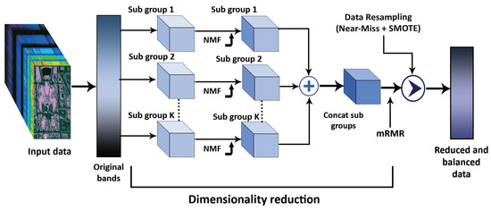
Figure 1.
The architecture of proposed subgrouping-based NMF method for dimensionality reduction.
In this way, only spectral bands that are essential for object recognition are eliminated, and reduction is carried out in a way that retains the intact spatial information. The HSI data cube is partitioned into tiny overlapping 3D patches, with the truth labels determined by the label of the patch’s center pixel, allowing it to be used with image classification methods. To encompass the window or geographical breadth and all R spectral bands, we generate the 3D adjacent patches from , with their centers at . With as input, can be used to determine the overall number of 3D patches that can be created. This is why the 3D patch at coordinates is written as ; it includes the space width from and height form . In this research, we suggest a modified network that can benefit from the automated feature learning capabilities of both 2D-CNNs and 3D-CNNs.
2.4. Proposed Deep Learning Model and Classification
The proposed approach utilizes a fusion of a 3D-CNN and 2D-CNN, allowing the extraction of significant spatial and spectral feature maps from the HSI in a cost-effective manner. The model design involves stacked 3D convolution layers followed by a decreasing dimension block that includes a Conv3D layer, reshaping operation, and another Conv3D layer. The resulting feature maps are reshaped and then processed through a Conv2D layer, which learns additional spatial features. The Conv2D layer’s output undergoes normalization before being passed to the first fully connected layer subsequent to the dropout layer. The overall proposed process is depicted in Figure 2 and Algorithm 2, both of which illustrate the unique architecture of the model. The proposed model comprises seven layers, starting with 3D convolutions (C1-C3) at levels one to three for extracting spectral–spatial information, followed by 2D convolutions (C4-C5) at the fourth and fifth levels, and finally two fully connected layers (F1-F2) at the end of the model. In a fully connected layer, each neuron communicates with all others in the layer beneath it and transmits the resulting value to the classifier. Pooling layers reduce the spatial resolution of images to reduce the size of feature maps and simplify calculations. The pooling layer does not store any extra data. According to the suggested architecture, each of the first three convolution layers uses a three-dimensional convolution kernel with dimensions of (i.e., ), (i.e., ), and (i.e., ), respectively; more specifically, implies 32 3D kernels of size (three dimensions, one spectral and two spatial) for each of the sixteen three-dimensional input feature maps. In order to perform 2D convolution processes, the data in the fourth layer must be a 3D image. When performing 2D convolution processes, it is first necessary to resize the input size to accommodate these procedures; -layer inputs are prepared, then a 2D convolution operation with kernel dimensions of (i.e., ) is performed on these inputs to generate 64 feature maps for the output of the fifth layer (i.e., 32 2D input feature maps are employed). The size of the following layer, which is part of the depthwise 2D convolution kernel, is (i.e., ). In order to counteract the issue of overfitting and enhance the rate at which the network converges, we integrate the batch normalization optimization method after every convolution layer. This strategic inclusion of batch normalization effectively mitigates overfitting, resulting in a more stable network. The adverse effects of overfitting are minimized by normalizing the output of each layer, leading to faster convergence and improved learning efficiency during the training process. In the end, all 256 neurons are linked to one another after the fifth layer is flattened. Table 1 provides a brief explanation of the proposed model, including information on the number of parameters, types of layers, and dimensions of the resulting maps. It is evident that the first thick layer (fully connected) has the greatest number of parameters. To account for each class included in a particular dataset, the deepest hidden layer has the same number of neurons. This means that the suggested model’s total number of parameters is class-specific. For the Salinas, Pavia University, and Kennedy Space Center datasets, the suggested model has 1,912,688, 1,911,785, and 1,912,430 trainable weight parameters, respectively. All weights start with a random value and are then taught via the backpropagation method, Adam optimizer, and Softmax classification.
| Algorithm 2 Dimensionality reduction. |
|
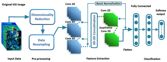
Figure 2.
The architecture of the proposed optimized 3D-2D CNN model for spectral–spatial feature extraction and classification.

Table 1.
Statistics of the SC dataset, including the name and number of total samples for each class.
3. Experiments
3.1. Dataset Description
- 1.
- Salinas Scene: the Salinas Scene (SC) dataset for HSIs was acquired in 1992 using the AVIRIS sensor, which obtained 566 images of the Salinas Valley in California. The initial image comprised 224 bands [39]. To create an HSI dataset with 204 bands, we excluded twenty water absorption bands: bands 108–112, 154–167, and 224. The spatial dimensions of the scene are pixels. The scene has a total of sixteen labeled classes. Figure 3a displays ground truth images of the SC dataset, and Table 1 shows the sample distributions for the experiment.
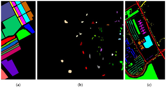 Figure 3. Ground truth images from the datasets: (a) SC, (b) KSC, and (c) PU.
 - 2.
- Pavia University: this dataset consists of ROSIS optical sensor data collected by the University of Pavia (PU) over the city of Pavia in northern Italy. The PU dataset has a spatial resolution of 1.3 m, and has 103 spectral bands in addition to its spatial resolution [39]. There are nine ground truth classes in PU. Further information on the PU experimental datasets may be accessed at [23]. Figure 3c displays the ground truth images for each of the experimental datasets. The sample distributions in the original dataset are shown in Figure 3c and Table 2.
 Table 2. Statistics of the PU dataset, including the name and number of total samples for each class.
 - 3.
- Kennedy Space Center: the final dataset, referred to as the Kennedy Space Center (KSC) dataset, was acquired on March 23, 1996 using the AVIRIS sensor, which captured the KSC region in Florida. This HSI dataset is characterized by spatial dimensions of pixels and comprises 224 spectral bands [39]. Following the removal of 48 noisy bands, a total of 172 spectral bands were obtained. The dataset consists of thirteen labeled classes, as outlined in Table 3. The sample distributions in the original dataset are shown in Figure 3b and Table 3.
 Table 3. Statistics of the KSC dataset, including the name and number of total samples for each class.
3.2. Experimental Setup and Hyperparameter Tuning
Before discussing the specifics of the experimental results, the different configurations of the deep learning approaches used in our research are described in depth. Each dataset contained distinct numbers of training and testing samples. Table 4 illustrates how the synthetic and real samples in the training data as well as the test samples are distributed after resampling. To achieve a fair comparison, we extracted the same spatial–spectral dimension in 3D patches of input volume for the different datasets, such as for all datasets. The article delves into the selection process for determining the window size of 3D patches, which has been concluded to be . This decision is supported by the results of a comprehensive window size analysis experiment, visually presented in Figure 4. Notably, this study revealed that a window size yields the highest accuracy. Furthermore, the top features selected using various dimensionality reduction techniques are showcased in Table 5. The data were then sent to the deep learning model. The model has a total of five convolution layers (three 3D-Conv and two 2D-Conv layers) and two fully connected layers. The suggested model is briefly described in Table 6, which includes details on the number of parameters, kinds of layers, and sizes of the resulting maps. The images are then classified using a Softmax layer with n classes, where n is the number of classes used across all datasets. In order to preserve as much data as possible for each pixel, the suggested network layout does not include pooling layers. Furthermore, we utilize Adam for network training, with a mini-batch size of 256 and a learning rate of 0.001. The training of the network lasts for a total of 120 epochs. During training, no extra data are utilized in any way. Two different sample ratios were used as the foundation for the investigations.

Table 4.
Training and testing sample data in detail for four datasets, including sample data.
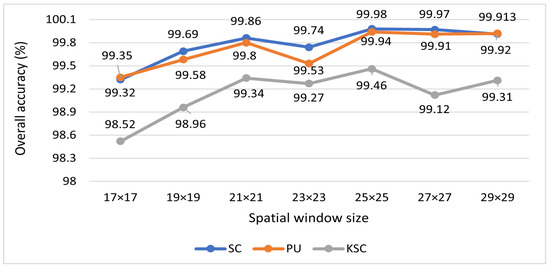
Figure 4.
The effect of varying the window size of the input cube on the proposed model’s accuracy for the SC, PU, and KSC datasets.

Table 5.
Selected features from the dataset by various dimensionality reduction methods.

Table 6.
A brief overview of the suggested model using a 25 × 25 window size.
The experimental design of the study involved two instances, in which 20% of the training data was separated from the testing data for validation purposes. The first instance consisted of a training and testing ratio of 10:90%, wherein 10% of the total data were allocated for training the model and 90% of the total data were reserved for testing the model’s performance. The second instance involved a training and testing ratio of 20:80%, wherein 20% of the total data were designated for training the model and 80% of the total data were used to assess the model’s performance. This approach of splitting the data into training, testing, and validation subsets helps in evaluating a machine learning model’s performance on unseen data and prevents overfitting of the model on the training data. Furthermore, the validation subset helps in fine-tuning the model’s parameters, enhancing the model’s generalization ability, and improving its predictive performance on new and unseen data. All experiments were implemented using the Tensorflow–Keras framework on Google Colab (Colab specs in brief: graphics processing unit (1xTesla K80) running compute version 3.7 with 2496 CUDA cores and 12GB of GDDR5 Virtual RAM; memory 12.68 GB; disk 78.19 GB). Google Colab IDE’s memory limits prevented us from running all the models with more than five features on this dataset.
3.3. Comparison Methods
- 1.
- SVM [40]: Mounika et al. used Principal Component Analysis (PCA) for feature extraction in the classification of hyperspectral images using Support Vector Machine (SVM). Their paper demonstrated the effectiveness of using PCA as a preprocessing technique for feature extraction in hyperspectral image classification, providing a valuable tool for researchers in remote sensing and image analysis.
- 2.
- 3D-CNN [27]: Li et al. proposed a 3D convolutional neural network (CNN) for spectral–spatial classification of hyperspectral images. Their paper introduced a novel method that utilizes both spectral and spatial information to improve classification performance. The application of 3D-CNNs for HSI classification can pose significant challenges in terms of computational requirements and data availability, potentially restricting its feasibility for certain practical applications.
- 3.
- Fast 3D-CNN [28]: Ahmad et al. introduced a fast and compact 3D-CNN for hyperspectral image classification that achieved high accuracy while using a relatively small number of parameters. This paper’s contribution lies in the development of an efficient method that overcomes the challenge of processing large amounts of hyperspectral data in real-time applications. A potential disadvantage of employing 3D-CNN for hyperspectral image classification is the risk of losing relevant information during the feature extraction process, which can negatively impact classification accuracy.
- 4.
- HybridSN [29]: HybridSN is a deep learning architecture proposed for efficient hyperspectral image classification. It combines a deep 2D CNN with a shallow 3D CNN to capture both spatial and spectral features of hyperspectral data. The architecture may pose a challenge in terms of hyperparameter tuning, as its performance can be highly dependent on the careful selection and adjustment of these parameters to achieve the best results.
- 5.
- SpectralNET [41]: this paper proposes a deep learning architecture that combines the spectral–spatial features of hyperspectral data with the multi-resolution analysis capabilities of wavelet transforms, with the aim of improving classification performance.
- 6.
- MDBA [42]: this paper’s main contribution lies in the development of a multibranch 3D Dense Attention Network (MDBA) that incorporates attention mechanisms to capture spatial and spectral information effectively. While the proposed MDBA offers promising results in hyperspectral image classification, it is important to note that the network architecture and attention mechanisms add complexity to the model, requiring careful implementation and large computational resources for practical deployment.
- 7.
- Hybrid 3D-CNN/2D-CNN [43]: In this paper, the authors proposed a hybrid CNN architecture combining 3D-CNN and 2D-CNN and using depthwise separable convolutions and group convolutions to improve the classification performance of hyperspectral images. However, the lack of comparison with state-of-the-art methods on larger or more diverse hyperspectral datasets makes it difficult to assess the generalizability and scalability of the proposed method beyond the specific conditions used in the study.
3.4. Complexity Analysis
To analyze the complexity of the proposed model, we can consider the number of parameters. Our developed model utilizes a customized hybrid CNN architecture. It consists of several convolutional layers followed by batch normalization, reshaping, and dense layers. The number of parameters in a CNN model depends on the architecture and the size of the layers. We can break down the number of parameters in each layer, using the example of the Salinas Scene dataset:
- 1.
- Conv3D Layer: the number of parameters in a Conv3D layer can be calculated as . The first Conv3D layer has eight filters and a kernel size of , and the input has one channel; thus, the number of parameters in this layer is parameters.
- 2.
- BatchNormalization Layer: the number of parameters in a BatchNormalization layer is equal to four times the number of filters in the previous layer. The first BatchNormalization layer after Conv3D has eight filters; thus, it has parameters.
- 3.
- Conv2D Layer: the number of parameters in a Conv2D layer can be calculated as . The Conv2D layer has 32 filters and a kernel size of , and the input has 32 channels; thus, the number of parameters in this layer is parameters.
- 4.
- DepthwiseConv2D Layer: the number of parameters in a DepthwiseConv2D layer can be calculated as . The DepthwiseConv2D layer has a kernel size of and 32 input channels; thus, the number of parameters in this layer is parameters.
- 5.
- Dense Layer: the number of parameters in a Dense layer can be calculated as . The first Dense layer has 256 units and an input dimension of 7200; thus, the number of parameters in this layer is parameters.
By summing up the number of parameters in each layer, we can find the total number of trainable parameters in the model, which is 1,912,688 parameters.
In comparison to the two most similar methods, “HybridSN” and “Hybrid 3D-2D CNN”, there are both similarities and differences. Both methods utilize a combination of 3D and 2D convolutions for feature extraction. However, the exact dimensions and configurations of the convolutional kernels differ. Regarding the “HybridSN” method, the convolutional kernels have dimensions of , and in the subsequent layers. Additionally, a 2D convolution with a kernel dimension of is applied before the flatten layer. The model consists of a total of 5,122,176 trainable weight parameters. The number of classes in the dataset determines the total number of parameters. On the other hand, the “Hybrid 3D-2D CNN” method comprises seven layers, starting with 3D convolutions and followed by 2D convolutions. The dimensions of the 3D convolution kernels are , , and . The output of the third layer is resized to fit the input size of the fourth layer, where a 2D convolution with a kernel dimension of is applied. A depthwise 2D convolution with a kernel dimension of is then performed. The model has a total of 1,033,728 trainable weight parameters.
When comparing the proposed model with the above two methods, it can be observed that the proposed model has a larger number of total and trainable parameters. This might indicate both higher model complexity and greater capacity to capture more intricate patterns and features. Additionally, the proposed model has a larger input shape , which could allow it to capture more spatial and spectral information from the data. These factors might contribute to the proposed model achieving better results compared to the other two methods, despite their lower number of trainable parameters. However, it is important to consider other factors, such as dataset characteristics, training settings, and evaluation metrics, when drawing a comprehensive comparison between the models.
3.5. Classification Performance
To assess the effectiveness of the proposed model, we selected three sets of freely accessible HSI data. We analyzed the impact of different dimensionality reduction methods on the accuracy of the proposed model, including PCA, Segmented PCA, MNF, Segmented MNF, Bg-MNF, NMF, and the dimensionality reduction method proposed in this paper. For the purpose of comparative analysis, we used state-of-the-art methods such as SVM [44], 3D CNN [27], Fast 3D CNN [28], HybridSN [29], SpectralNET [41], Hybrid 3D 2D CNN [43], etc. Our proposed approach demonstrates superior performance compared to other dimensionality reduction methods when evaluated on these deep learning model. Figure 5, Figure 6, Figure 7, Figure 8, Figure 9 and Figure 10 provide a detailed analysis and comparison of our method with existing approaches, highlighting its advantages in terms of accuracy and loss metrics for both training and validation data. Additionally, we employed performance measurements such as the overall accuracy (OA), average accuracy (AA) for each class, and Kappa coefficient (Kappa). The OA measure considers the ratio of properly categorized images in the testing dataset to the total number of samples, the AA metric indicates the mean of the accuracy of the image class, and the Kappa metric indicates the weighting of the observed accuracy. Both metrics are used to quantify image quality. Precision, recall, and f-1 score are other kinds of commonly used performance metrics, with their weighted averages being used here as the weighted average can provide more reliable results than a simple average. To calculate the weighted averages, the value of each data point is first multiplied by the weight associated with it, then the resulting total is divided by the number of datapoints.
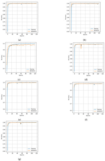
Figure 5.
Accuracy curves for training and validation data of SC dataset obtained with different dimensionality reduction methods: (a) PCA, (b) Segmented PCA, (c) MNF, (d) Segmented MNF, (e) Bg-MNF, (f) NMF, (g) proposed method (SNC).
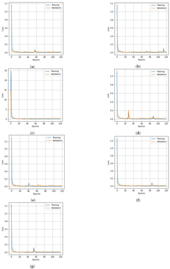
Figure 6.
Loss curve for training and validation data of SC dataset obtained from different dimensionality reduction methods: (a) PCA, (b) Segmented PCA, (c) MNF, (d) Segmented MNF, (e) Bg-MNF, (f) NMF, (g) proposed method (SNC).
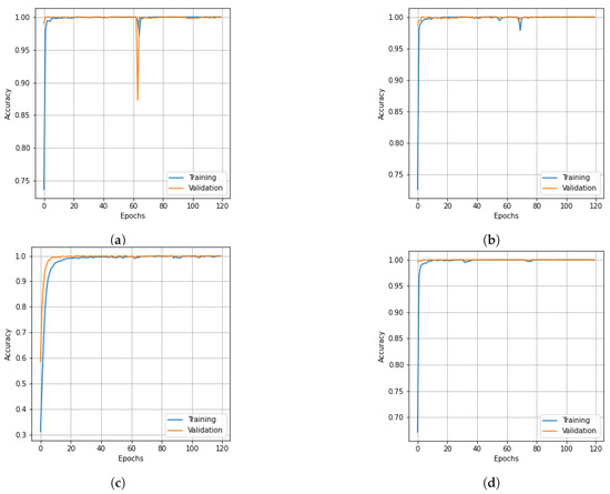
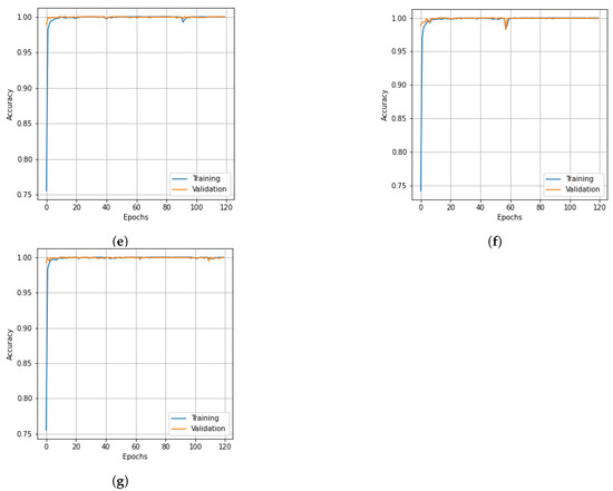
Figure 7.
Accuracy curves for training and validation data of the PU dataset obtain obtained with different dimensionality reduction methods: (a) PCA, (b) Segmented PCA, (c) MNF, (d) Segmented MNF, (e) Bg-MNF, (f) NMF, (g) proposed method (SNC).
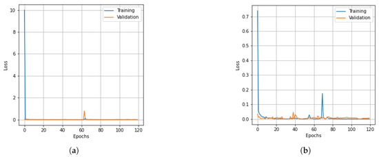
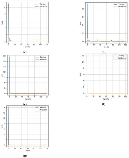
Figure 8.
Loss curves for training and validation data of the PU dataset obtained with different dimensionality reduction methods. (a) PCA, (b) Segmented PCA, (c) MNF, (d) Segmented MNF, (e) Bg-MNF, (f) NMF, (g) proposed method (SNC).
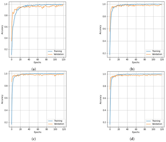
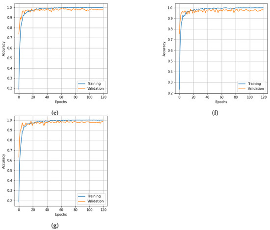
Figure 9.
Accuracy curves for training and validation data of KSC dataset obtained with different dimensionality reduction methods: (a) PCA, (b) Segmented PCA, (c) MNF, (d) Segmented MNF, (e) Bg-MNF, (f) NMF, (g) proposed method (SNC).
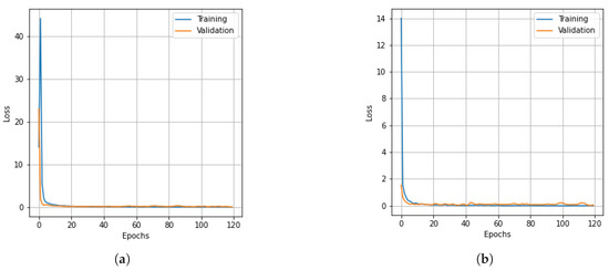
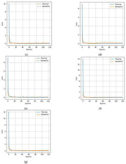
Figure 10.
Loss curves for training and validation data of the KSC dataset obtain with different dimensionality reduction methods: (a) PCA, (b) Segmented PCA, (c) MNF, (d) Segmented MNF, (e) Bg-MNF, (f) NMF, (g) proposed method (SNC).
On the basis of the different datasets, we describe the experimental results in different domains of analysis. We note that the OA of the suggested SNC model is greater than 99% in every dataset, resulting in the best performance. In each classification table, the most significant values are bolded; additionally, according to the findings of our experiment, the classification of HSI requires a greater emphasis on spatial context than on spectral correlations.
3.5.1. Results for the SC
The structure of the deep learning models in this experiment were quite similar to those mentioned in the experimental setup, with the only variation being the number of parameters that were altered following parameter tuning, such as the threshold value for segmentation and the number of spatial features after reduction. On the basis of the SC dataset and using training data of 10% and 20%, Table 7 shows the experimental outcomes and effects of several resampling techniques. We used a number of different dimensionality reduction techniques; this analysis is shown in Table 8 along with the results for the proposed method. Table 9 illustrates how the size of the spatial window affects the overall accuracy and training time. Finally, the experimental outcomes of all state-of-the-art strategies tested on the SC dataset are summarized in Table 10. The SNC model’s OA is 99.98%. Figure 5 and Figure 6 show the categorization outcomes for each comparative technique as accuracy and loss curves, respectively. The accuracy and loss curves shown here were produced with both training samples and validation samples, Figure 5g and Figure 6g demonstrate the optimum performance.

Table 7.
Classification accuracy (%) for the SC dataset using different resampling techniques with the proposed SNC model.

Table 8.
Effects of different dimensionality reduction methods on the proposed deep learning model.

Table 9.
Effects of different window sizes on the overall accuracy and training time for the SC dataset.

Table 10.
Classification accuracy (in percentage) of the proposed model compared to state-of-the-art methods on the SC dataset.
3.5.2. Results for the PU
The results of the experiments as well as the impacts of the various resampling methods are presented in Table 11. In addition to this, we employed a variety of methods for dimensionality reduction; the analysis is presented in Table 12 alongside the findings obtained using the suggested approach. Table 13 provides a concise summary of the results of the experiments conducted on the state-of-the-art techniques that were evaluated using the PU dataset. The OA of the SNC model is 99.98%. Accuracy and loss curves illustrating the results of categorization are presented in Figure 7 and Figure 8, respectively, for each of the comparing techniques. The accuracy and loss curves were generated using both training data and validation samples. The best possible optimal performance in terms of accuracy and loss is depicted in Figure 7g and Figure 8g, respectively. Table 14 demonstrates how the overall accuracy and the amount of time required for training can be affected by the size of the spatial window.

Table 11.
Classification accuracy (%) for the PU Dataset using different resampling techniques with the proposed SNC model.

Table 12.
Effects of different dimensionality reduction methods on the proposed deep learning model for PU dataset.

Table 13.
Classification accuracy (in percentage) of the proposed model compared to state-of-the-art methods on the PU dataset.

Table 14.
Effects of different window sizes on the proposed method’s overall accuracy and training time for the PU dataset.
3.5.3. Results for the KSC
As in the earlier scenes, we only modified a few parameters from the deep learning model discussed in the experimental configuration. Table 15 presents the experimental results of all the methods based on the KSC dataset without resampling and after data resampling. The impacts of different dimensionality reduction techniques and window sizes of cube patches are shown in Table 16 and Table 17, respectively. The experimental findings of the evaluations of the state-of-the-art methods on the KSC dataset are summarized in Table 18. The OA, Kappa, and AA of the SNC model are 99.46%, 99.41%, and 99.43% respectively. The proposed SNC model outperforms the other methods. The graphs in Figure 9 and Figure 10 demonstrate the correlation between the loss value and classification accuracy of the KSC dataset during the training iteration epochs. The curves reveal that the loss values for all three spatial strategies stabilize after roughly 120 training iteration epochs, and this trend is mirrored in the accuracy variation over the training iteration epochs.

Table 15.
Classification accuracy (%) for the KSC dataset using different resampling techniques with the proposed SNC model.

Table 16.
Effects of different dimensionality reduction methods on the proposed deep learning model for the KSC dataset.

Table 17.
Effects of different window sizes on overall accuracy and training time for the KSC dataset.

Table 18.
Classification accuracy (in percentage) of the proposed model compared to state-of-the-art methods on the KSC dataset.
The results of the experiment showcased in Figure 11 aim to evaluate the performance of the proposed model in comparison to different state-of-the-art methods. The experiment demonstrates the superiority of our model, as reflected by the accuracy and loss curves, reaffirming its effectiveness in achieving improved results. The findings from this experiment highlight the potential of our approach and its ability to outperform existing methods in terms of accuracy and convergence rate.
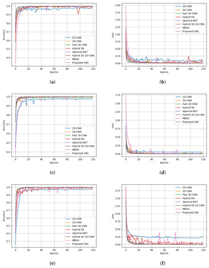
Figure 11.
Accuracy and loss curves for training epochs obtained from state-of-the-art methods. Salinas dataset: (a) accuracy and (b) loss curves; Pavia University dataset: (c) accuracy and (d) loss curves; KSC dataset: (e) accuracy and (f) loss curves.
4. Conclusions and Future Work
In this article, we propose a hybrid deep learning-based model for the extraction of features and recognition of objects from unbalanced Hyperspectral Imaging (HSI) data. The suggested model uses a resampling method to address the class imbalance problem and maintain the equilibrium of the model’s performance metrics. The proposed approach considers the overall properties of the data for feature extraction, using correlation as the preferred metric for measuring mutual information between HSI bands. The presented method facilitates a new form of subgrouping-based dimensionality reduction of the original data, thereby lowering the processing time required for complete subgrouping. Additionally, the study introduces a 3D-CNN and 2D-CNN hybrid model for object classification in HSI which combines spatial and spectral characteristics to enhance classification accuracy. The incorporation of both 3D and 2D convolutions makes the hybrid model more computationally efficient, requiring fewer learning parameters than 3D-CNN alone. Together, the presented approaches (SNC model) perform better than the baselines in terms of error rate, which is a common metric for evaluating per-pixel object classification performance.
Future research in this field could focus on incorporating past domain information into the proposed deep learning model. Moreover, transfer learning approaches could be investigated to address the limitations of the current deep learning model, which requires significantly more data for training than alternatives built using more conventional machine learning techniques. Overall, the suggested hybrid deep learning-based model holds great potential for improving the recognition of objects from unbalanced HSI data, and further research in this area could lead to significant advancements in this field.
Author Contributions
Conceptualization, M.T.I. and M.R.I.; methodology, M.T.I. and M.R.I.; software, M.T.I. and M.R.I.; validation, M.T.I., M.R.I. and M.P.U.; formal analysis, M.R.I., M.P.U. and A.U.; investigation, M.P.U. and A.U.; resources, M.T.I., M.R.I. and M.P.U.; data curation, M.T.I. and M.R.I.; writing—original draft preparation, M.T.I. and M.R.I.; writing—review and editing, M.P.U. and A.U.; visualization, M.T.I. and M.R.I.; supervision, M.R.I., M.P.U. and A.U.; funding acquisition, M.P.U. and A.U. All authors have read and agreed to the published version of this manuscript.
Funding
This research received no external funding.
Institutional Review Board Statement
Not applicable.
Informed Consent Statement
Not applicable.
Data Availability Statement
The data experimented on in this study are available in [45].
Conflicts of Interest
The authors declare no conflict of interest.
References
- Zhao, J.L.; Lerner, A.; Shu, Z.; Gao, X.J.; Zee, C.S. Imaging spectrum of neurocysticercosis. Radiol. Infect. Dis. 2015, 1, 94–102. [Google Scholar] [CrossRef]
- Mallapragada, S.; Wong, M.; Hung, C.C. Dimensionality reduction of hyperspectral images for classification. In Proceedings of the Ninth International Conference on Information, Tokyo, Japan, 9–12 October 2018; Volume 1. [Google Scholar]
- Yuen, P.W.; Richardson, M. An introduction to hyperspectral imaging and its application for security, surveillance and target acquisition. Imaging Sci. J. 2010, 58, 241–253. [Google Scholar] [CrossRef]
- Lv, W.; Wang, X. Overview of hyperspectral image classification. J. Sens. 2020, 2020. [Google Scholar] [CrossRef]
- Uddin, M.P.; Mamun, M.A.; Hossain, M.A. PCA-based feature reduction for hyperspectral remote sensing image classification. IETE Tech. Rev. 2021, 38, 377–396. [Google Scholar] [CrossRef]
- Jayaprakash, C.; Damodaran, B.B.; Sowmya, V.; Soman, K. Dimensionality reduction of hyperspectral images for classification using randomized independent component analysis. In Proceedings of the 2018 5th IEEE International Conference on Signal Processing and Integrated Networks (SPIN), Noida, India, 22–23 February 2018; pp. 492–496. [Google Scholar]
- Boori, M.S.; Paringer, R.A.; Choudhary, K.; Kupriyanov, A.V. Comparison of hyperspectral and multi-spectral imagery to building a spectral library and land cover classification performanc. Comput. Opt. 2018, 42, 1035–1045. [Google Scholar] [CrossRef]
- Aparna, G.; Rachana, K.; Rikhita, K.; Phaneendra Kumar, B.L. Comparison of Feature Reduction Techniques for Change Detection in Remote Sensing. In Evolution in Signal Processing and Telecommunication Networks, Proceedings of Sixth International Conference on Microelectronics, Electromagnetics and Telecommunications (ICMEET 2021), Bhubaneswar, India, 27–28 August 2021; Springer: Berlin, Germnay, 2022; Volume 2, pp. 325–333. [Google Scholar]
- Rodarmel, C.; Shan, J. Principal component analysis for hyperspectral image classification. Surv. Land Inf. Sci. 2002, 62, 115–122. [Google Scholar]
- Luo, G.; Chen, G.; Tian, L.; Qin, K.; Qian, S.E. Minimum noise fraction versus principal component analysis as a preprocessing step for hyperspectral imagery denoising. Can. J. Remote Sens. 2016, 42, 106–116. [Google Scholar] [CrossRef]
- Du, Q.; Zhu, W.; Yang, H.; Fowler, J.E. Segmented principal component analysis for parallel compression of hyperspectral imagery. IEEE Geosci. Remote Sens. Lett. 2009, 6, 713–717. [Google Scholar]
- Lixin, G.; Weixin, X.; Jihong, P. Segmented minimum noise fraction transformation for efficient feature extraction of hyperspectral images. Pattern Recognit. 2015, 48, 3216–3226. [Google Scholar] [CrossRef]
- Tsuge, S.; Shishibori, M.; Kuroiwa, S.; Kita, K. Dimensionality reduction using non-negative matrix factorization for information retrieval. In Proceedings of the 2001 IEEE International Conference on Systems, Man and Cybernetics. e-Systems and e-Man for Cybernetics in Cyberspace (Cat. No. 01CH37236), Tucson, AZ, USA, 7–10 October 2001; Volume 2, pp. 960–965. [Google Scholar]
- Wu, L.; Kong, C.; Hao, X.; Chen, W. A short-term load forecasting method based on GRU-CNN hybrid neural network model. Math. Probl. Eng. 2020, 2020, 1–10. [Google Scholar] [CrossRef]
- Liu, G.; Xiao, L.; Xiong, C. Image classification with deep belief networks and improved gradient descent. In Proceedings of the 2017 IEEE International Conference on Computational Science and Engineering (CSE) and IEEE International Conference on Embedded and Ubiquitous Computing (EUC), Guangzhou, China, 21–24 July 2017; Volume 1, pp. 375–380. [Google Scholar]
- Farrell, M.D.; Mersereau, R.M. On the impact of PCA dimension reduction for hyperspectral detection of difficult targets. IEEE Geosci. Remote Sens. Lett. 2005, 2, 192–195. [Google Scholar] [CrossRef]
- Van Der Maaten, L.; Postma, E.; Van den Herik, J. Dimensionality reduction: A comparative. J. Mach. Learn. Res. 2009, 10, 13. [Google Scholar]
- Du, Q.; Chang, C.I. Segmented PCA-based compression for hyperspectral image analysis. In Proceedings of the Chemical and Biological Standoff Detection; SPIE: Bellingham, WA, USA, 2004; Volume 5268, pp. 274–281. [Google Scholar]
- Chen, G.; Qian, S.E. Evaluation and comparison of dimensionality reduction methods and band selection. Can. J. Remote Sens. 2008, 34, 26–36. [Google Scholar] [CrossRef]
- Zhang, Z.Y. Nonnegative matrix factorization: Models, algorithms and applications. Data Mining Found. Intell. Paradig. 2012, 2, 99–134. [Google Scholar]
- Kumar, N.; Uppala, P.; Duddu, K.; Sreedhar, H.; Varma, V.; Guzman, G.; Walsh, M.; Sethi, A. Hyperspectral tissue image segmentation using semi-supervised NMF and hierarchical clustering. IEEE Trans. Med Imaging 2018, 38, 1304–1313. [Google Scholar] [CrossRef]
- Harikiran, J.J.H. Hyperspectral image classification using support vector machines. IAES Int. J. Artif. Intell. 2020, 9, 684. [Google Scholar] [CrossRef]
- Petersson, H.; Gustafsson, D.; Bergstrom, D. Hyperspectral image analysis using deep learning—A review. In Proceedings of the 2016 IEEE Sixth International Conference on Image Processing Theory, Tools and Applications (IPTA), Oulu, Finland, 12–15 December 2016; pp. 1–6. [Google Scholar]
- Rissati, J.; Molina, P.; Anjos, C. Hyperspectral image classification using random forest and deep learning algorithms. In Proceedings of the 2020 IEEE Latin American GRSS & ISPRS Remote Sensing Conference (LAGIRS), Santiago, Chile, 22–26 March 2020; p. 132. [Google Scholar]
- Vaddi, R.; Manoharan, P. Hyperspectral image classification using CNN with spectral and spatial features integration. Infrared Phys. Technol. 2020, 107, 103296. [Google Scholar] [CrossRef]
- Medus, L.D.; Saban, M.; Frances-Villora, J.V.; Bataller-Mompean, M.; Rosado-Muñoz, A. Hyperspectral image classification using CNN: Application to industrial food packaging. Food Control 2021, 125, 107962. [Google Scholar] [CrossRef]
- Li, Y.; Zhang, H.; Shen, Q. Spectral-spatial classification of hyperspectral imagery with 3D convolutional neural network. Remote Sens. 2017, 9, 67. [Google Scholar] [CrossRef]
- Ahmad, M.; Khan, A.M.; Mazzara, M.; Distefano, S.; Ali, M.; Sarfraz, M.S. A fast and compact 3-D CNN for hyperspectral image classification. IEEE Geosci. Remote Sens. Lett. 2020, 19, 1–5. [Google Scholar] [CrossRef]
- Roy, S.K.; Krishna, G.; Dubey, S.R.; Chaudhuri, B.B. HybridSN: Exploring 3-D–2-D CNN feature hierarchy for hyperspectral image classification. IEEE Geosci. Remote Sens. Lett. 2019, 17, 277–281. [Google Scholar] [CrossRef]
- Kotsiantis, S.; Kanellopoulos, D.; Pintelas, P. Handling imbalanced datasets: A review. GESTS Int. Trans. Comput. Sci. Eng. 2006, 30, 25–36. [Google Scholar]
- Sun, Y.; Wong, A.K.; Kamel, M.S. Classification of imbalanced data: A review. Int. J. Pattern Recognit. Artif. Intell. 2009, 23, 687–719. [Google Scholar] [CrossRef]
- Chaubey, Y.P. Resampling methods: A practical guide to data analysis. Technometrics 2000, 42, 311. [Google Scholar] [CrossRef]
- Somasundaram, A.; Reddy, U.S. Data imbalance: Effects and solutions for classification of large and highly imbalanced data. In Proceedings of the 1st International Conference on Research in Engineering, Computers and Technology (ICRECT 2016), Tiruchirappalli, India, 8–10 September 2016. [Google Scholar]
- Liu, B.; Tsoumakas, G. Dealing with class imbalance in classifier chains via random undersampling. Knowl.-Based Syst. 2020, 192, 105292. [Google Scholar] [CrossRef]
- Zheng, Z.; Cai, Y.; Li, Y. Oversampling method for imbalanced classification. Comput. Inform. 2015, 34, 1017–1037. [Google Scholar]
- Chawla, N.V.; Bowyer, K.W.; Hall, L.O.; Kegelmeyer, W.P. SMOTE: Synthetic minority over-sampling technique. J. Artif. Intell. Res. 2002, 16, 321–357. [Google Scholar] [CrossRef]
- Alsowail, R.A. An Insider Threat Detection Model Using One-Hot Encoding and Near-Miss Under-Sampling Techniques. In Proceedings of the International Joint Conference on Advances in Computational Intelligence: IJCACI 2021, online, 23–24 October 2021; Springer: Berlin, Germany, 2022; pp. 183–196. [Google Scholar]
- Borgognone, M.G.; Bussi, J.; Hough, G. Principal component analysis in sensory analysis: Covariance or correlation matrix? Food Qual. Prefer. 2001, 12, 323–326. [Google Scholar] [CrossRef]
- Billah, M.; Waheed, S. Minimum redundancy maximum relevance (mRMR) based feature selection from endoscopic images for automatic gastrointestinal polyp detection. Multimed. Tools Appl. 2020, 79, 23633–23643. [Google Scholar] [CrossRef]
- Tsai, F.; Lin, E.K.; Yoshino, K. Spectrally segmented principal component analysis of hyperspectral imagery for mapping invasive plant species. Int. J. Remote Sens. 2007, 28, 1023–1039. [Google Scholar] [CrossRef]
- Chakraborty, T.; Trehan, U. Spectralnet: Exploring spatial-spectral waveletcnn for hyperspectral image classification. arXiv 2021, arXiv:2104.00341. [Google Scholar]
- Yin, J.; Qi, C.; Huang, W.; Chen, Q.; Qu, J. Multibranch 3d-dense attention network for hyperspectral image classification. IEEE Access 2022, 10, 71886–71898. [Google Scholar] [CrossRef]
- Diakite, A.; Jiangsheng, G.; Xiaping, F. Hyperspectral image classification using 3D 2D CNN. IET Image Process. 2021, 15, 1083–1092. [Google Scholar] [CrossRef]
- Mounika, K.; Aravind, K.; Yamini, M.; Navyasri, P.; Dash, S.; Suryanarayana, V. Hyperspectral image classification using SVM with PCA. In Proceedings of the 2021 6th IEEE International Conference on Signal Processing, Computing and Control (ISPCC), Solan, India, 7–9 October 2021; pp. 470–475. [Google Scholar]
- Graña, M.; Veganzons, M.; Ayerdi, B. Hyperspectral Remote Sensing Scenes. 2021. Available online: https://www.ehu.eus/ccwintco/index.php/Hyperspectral_Remote_Sensing_Scenes (accessed on 11 July 2023).
Disclaimer/Publisher’s Note: The statements, opinions and data contained in all publications are solely those of the individual author(s) and contributor(s) and not of MDPI and/or the editor(s). MDPI and/or the editor(s) disclaim responsibility for any injury to people or property resulting from any ideas, methods, instructions or products referred to in the content. |
© 2023 by the authors. Licensee MDPI, Basel, Switzerland. This article is an open access article distributed under the terms and conditions of the Creative Commons Attribution (CC BY) license (https://creativecommons.org/licenses/by/4.0/).