
A Novel Forest EcoSpatial Network for Carbon Stocking Using Complex Network Theory in the Yellow River Basin


State Forestry and Grassland Administration Key Laboratory of Forest Resources & Environmental Management, Beijing Forestry University, Beijing 100083, China
*
Author to whom correspondence should be addressed.
Remote Sens. 2023, 15(10), 2612; https://doi.org/10.3390/rs15102612
Submission received: 4 April 2023
/
Revised: 10 May 2023
/
Accepted: 15 May 2023
/
Published: 17 May 2023
(This article belongs to the Special Issue Editorial Board Members’ Collection Series: Forest Environment Monitoring Based on Multi-Source Remote Sensing Data)
Abstract
:The Yellow River Basin serves as a crucial ecological barrier in China, emphasizing the importance of accurately examining the spatial distribution of forest carbon stocks and enhancing carbon sequestration in order to attain “carbon peaking and carbon neutrality”. Forest patches have complex interactions that impact ecosystem services. To our knowledge, very few studies have explored the connection between these interactions and carbon stock. This study addressed this gap by utilizing complex network theory to establish a forest ecospatial network (ForEcoNet) in the Yellow River Basin in which forest patches are represented as nodes (sources) and their interactions as edges (corridors). Our objective was to optimize the ForEcoNet’s structure and enhance forest carbon stocks. First, we employed downscaling technology to allocate the forest carbon stocks of the 69 cities in the study area to grid cells, generating a spatial distribution map of forest carbon density in the Yellow River Basin. Next, we conducted morphological spatial pattern analysis (MSPA) and used the minimum cumulative resistance model (MCR) to extract the ForEcoNet in the basin. Finally, we proposed optimization of the ForEcoNet based on the coupling coordination between the node carbon stock and topological structure. The results showed that: (1) the forest carbon stocks of the upper, middle, and lower reaches accounted for 42.35%, 54.28%, and 3.37% of the total, respectively, (2) the ForEcoNet exhibited characteristics of both a random network and a scale-free network and demonstrated poor network stability, and (3) through the introduction of 51 sources and 46 corridors, we optimized the network and significantly improved its robustness. These findings provide scientific recommendations for the optimization of forest allocation in the Yellow River Basin and achieving the goal of increasing the forest carbon stock.
1. Introduction
Global climate change has become one of the biggest challenges for human development and poses a significant threat to global human society. In order to avoid extreme harm and reduce the extent of global warming, “carbon peaking” and “carbon neutrality” have become long-term goals under the context of global warming [1]. There are two methods to become carbon neutral: reducing emissions and increasing carbon sequestration. The Intergovernmental Panel on Climate Change (IPCC) emphasized, in its special report, the necessity of reducing and gradually eliminating the use of fossil fuels and encouraging the use of renewable energy sources. In addition, to attain sustainable development and net-zero carbon emissions, it is crucial to promote carbon sequestration in both terrestrial and marine ecosystems [2]. Forests constitute the largest carbon reservoir in terrestrial ecosystems, fixing CO2 from the air in the form of biomass in plants and soil and thus playing a vital role in sequestering carbon. Forests maintain more than 80% of the world’s vegetation carbon reserves and approximately 40% of the global soil carbon reservoir [3,4]. Annually, approximately two-thirds of carbon in the terrestrial ecosystem can be attributed to forests [5]. Therefore, accurately exploring the spatial distribution of forest carbon stock and the potential for forest carbon sequestration is indispensable for regulating global carbon balance, mitigating the rise in concentrations of greenhouse gases such as CO2 in the atmosphere, and sustaining the overall global climate.
The spatial distribution of forest carbon stock can reflect the overall carbon stock situation in a region and offer initial values for process-based carbon cycling models to simulate carbon dynamics [6]. By combining forest inventory data with remote sensing technology, the spatial inversion of forest carbon stock can effectively integrate the accuracy of field measurements and the spatial distribution information obtained through remote sensing [7,8]. Previous studies have demonstrated the significant influence of geographic and climatic factors on the spatial distribution of forest carbon stock [9,10], as well as the variation in carbon sequestration capabilities among different tree species and forest ages [11,12]. In addition, the landscape pattern and heterogeneity of forests are closely related to ecological functions [13]. Although the relationship between forest structure, environmental factors, landscape patterns, and forest carbon storage has been gradually revealed in recent years, research on the relationship between forest patches and carbon stock is still limited. These patch-to-patch interactions can be referred to as topological structures [14]. Traditional landscape pattern analysis methods cannot verify whether the interactions between patches will affect carbon storage, and how they may affect it, while complex network theory provides us with a new perspective.
Complex networks are the results of the abstraction of complex systems by treating all components of the system as nodes and representing their interactions through interconnected edges [15]. Complex networks have been widely used to describe the network structures and evolution rules in fields such as the social, medical, and biological sciences [16,17,18]. When complex networks are applied to landscape ecology, ecospatial networks are formed [19]. Ecospatial networks consist of ecological sources and corridors, the former being patches that provide multiple ecosystem services, maintain ecosystem stability, and make important contributions to ecosystem development while the latter represent the structures of relationships between objects and carry out functions such as information transmission, material circulation, and energy flow [20]. Unlike the method of describing the overall characteristics of a region with landscape pattern indices, the methods used by ecospatial networks place more emphasis on the topological characteristics of a region, which have been shown to have an impact on ecosystem services [21]. Some studies have already optimized ecological networks to enhance ecosystem services [22,23]. Most of them focused on urban or national scales and used empirical models to quantify ecosystem services: a methodology which is feasible at small or large scales. However, at the basin scale, where climate and geography vary greatly, this quantification method lacks reliability. Furthermore, although previous studies have proposed optimization measures such as increasing forest sources and corridors, they have difficulty providing detailed quantitative data to support these measures due to a lack of specific optimization standards and actual vegetation data.
Therefore, this paper proposes a novel forest ecospatial network (ForEcoNet) based on complex network theory to achieve the increasing of forest carbon stock. Firstly, in our study, we calibrated the forest density distribution map of the Yellow River Basin and then combined forest inventory data to achieve the spatial grid mapping of forest carbon density in each city. Secondly, the ForEcoNet of the Yellow River Basin was extracted and evaluated using topological indicators. Finally, quantitative measures to optimize ForEcoNet for carbon stocking in the study area were proposed based on a coupling coordination analysis. This study’s results are important for monitoring forest structure and carbon storage distribution, and can provide scientific reference for strengthening the scientific management of forest ecosystems and formulating specific measures for carbon sequestration in the region.
2. Materials and Methods
2.1. Study Area
The Yellow River, with a total length of 5464 km, runs through nine provinces, including Qinghai, Sichuan, Gansu, Ningxia, Inner Mongolia, Shaanxi, Shanxi, Henan, and Shandong, originating from the Bayan Har Mountains of Qinghai Province [24]. This study is based on the natural geographical unit of the Yellow River Basin, and on the premise of ensuring the integrity of the urban spatial unit, the 69 cities that the mainstream Yellow River passes through are divided within the Yellow River Basin according to administrative boundaries (Figure 1). The upper reaches of the river flow through five provinces and 28 cities from the source to the mouth in the Hegou town of Inner Mongolia, accounting for 74.24% of the total basin area. The middle reaches flow through four provinces and 26 cities from Hegou town to Taohuayu in Zhengzhou, Henan, accounting for 19.80% of the total basin area. The lower reaches flow through two provinces and 15 cities from Taohuayu to the Bohai Sea, accounting for 5.96% of the total basin area. The Yellow River Basin covers a vast area with different terrain and landforms in the upper, middle, and lower reaches. It spans three major topographical steps and four major geomorphic units from west to east [25]. The climate within the basin varies significantly, with the southeastern, central, and northwestern regions belonging to semi-humid, semi-arid, and arid climate zones, respectively [26]. The vegetation in the Yellow River Basin is influenced by both horizontal zonality and monsoons, spanning four vegetation zones from east to west including the deciduous broad-leaved forest zone, grassland zone, desert zone, and Qinghai-Tibet Plateau vegetation zone [27].
2.2. Data Sources and Processing
In this study, we utilized the forest aboveground carbon stock and forest coverage data of 69 cities within the Yellow River Basin. These data were provided by the National Forestry and Grassland Administration based on their continuous forest inventory. The forest density map at a resolution of 1 km was derived by overlaying density datasets for different forest types (2020) including the 1-km arbor forest density dataset [28], 1-km bamboo forest density dataset [29], and 1-km mangrove forest density dataset [30]. In addition, we obtained factor data necessary for constructing ecological resistance surface, including land cover data, nighttime light data, normalized difference vegetation index (NDVI) data, modified normalized difference water index (MNDWI) data, digital elevation model (DEM) data, road network, water network, and population data (Table 1). To ensure consistency with the resolution of the forest density map, all resistance factor data were resampled to a resolution of 1 km using the nearest neighbor resampling. Administrative boundary data were provided by the Resource and Environmental Science and Data Center of the Chinese Academy of Sciences (https://www.resdc.cn/, accessed on 17 November 2022).
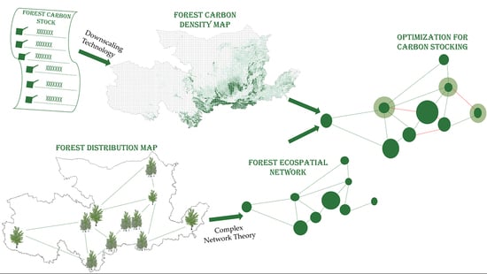
The study was conducted in three parts (Figure 2). In the first part, we allocated the forest carbon stocks of the 69 cities within the study area to the respective grid cells using conversion functions between the calibrated forest cover map, NDVI, and carbon stock. In the second part, we extracted ecological sources from the forest density map and conducted an ecological resistance surface to delineate the ecological spatial network. In the third part, we optimized theForEcoNet based on the coupling coordination results between the topological importance and carbon sequestration capacity of nodes.
2.3. Forest Carbon Mapping in the Yellow River Basin
2.3.1. Forest Area Calibration
The forest area obtained through a forest inventory is highly accurate, while remote sensing data provide spatial distribution information on forest density. However, due to limitations in resolution and potential deviations during the acquisition and processing of remote sensing data, the forest area calculated through remote sensing may differ from the actual area. Additionally, discrepancies in forest definitions and threshold divisions between the two methods may result in regional variances in the data. To address these issues, this study utilized the approach developed by Päivinen for forest area calibration [31]. The primary idea behind this approach is to adjust the proportion of forest and non-forest cover for each pixel in order to progressively minimize the difference between the forest density map and forest inventory coverage.
where stands for each pixel, is the total number of pixels in each city used to calibrate the forest density map, stands for the land cover type within each pixel (which is divided into forest () and non-forest ()), is the percentage of land cover type in pixel (e.g., is the forest cover proportion of the pixel , which is directly from the forest density map), is the average density of type estimated from the forest density map in the city, is the coverage of land cover type in the same city based on the forest inventory, is the correction coefficient for type , is the corrected forest cover proportion of pixel for land type , and is the sum of the correction ratios of the two land cover types within pixel . The scaled pixel ensures that the sum of the coverage ratios of the forest or non-forest within each pixel is equal to 1. is the proportion of land cover type after correction and scaling in pixel , is the average density of type after correction and scaling in the entire city, and represents the calibration threshold, which was set to 0.01 in this study, indicating that the calibration process was repeated until was less than 0.01. To avoid situations where the difference between the forest density map and the forest inventory coverage was too large to be corrected, the maximum number of iterations was limited to 100.
2.3.2. Mapping of Forest Carbon Stock Based on Downscaling Technology
In this study, downscaling technology was used to allocate forest carbon stocks at the city scale to grid cells, thereby incorporating spatial information. Previous research has demonstrated that forest carbon stock is associated with forest cover area and NDVI values at the national, provincial, and county scales [8]. The forest carbon stock in the 69 cities within the study area is directly proportional to the product of the total (the sum of “forest coverage * NDVI”) forest coverage area and NDVIs of each city (Figure S1). Using the calibrated forest density map and NDVI distribution map as a link, the study established a conversion function between the carbon stock of each spatial grid and the corresponding forest cover ratio and NDVI of the grid. Through this approach, carbon stocks at the city level could be allocated to 1-km grid cells, as depicted below:
where represents the forest carbon stock density of pixel , is the number of pixels in a city, is the total forest carbon stock in a city, is the proportion of forest area in corrected maps at pixel , matched with inventory data, represents the NDVI value (−1, 1) within pixel , and is the area of the pixel (100 ha).
2.4. Development of Forest Ecospatial Network in the Yellow River Basin
2.4.1. Extraction of Ecological Sources
Morphological spatial pattern analysis (MSPA) is a spatial pattern analysis method that focuses on measuring structural connectivity and can effectively identify important habitat patches in a study area [32]. We used the forest density map as input data and categorized patches with a forest density of 0 as background, while patches with forest densities greater than 0 were considered foreground. After classifying the foreground and background, MSPA employs a range of image processing techniques and mathematical operations, such as expansion reconstruction and skeleton extraction, to classify the foreground into seven distinct categories [33]. These categories are the core, islet, perforation, edge, bridge, loop, and branch (Table 2), and the core was regarded as the ecological source in this study.
2.4.2. Construction of Ecological Cumulative Resistance Surface and Ecological Corridors
A resistance surface is a simulated surface that represents the degree of difficulty of species migration in a real environment. The ecological resistance surface estimates the resistance that ecological patches encounter during the process of information transfer, material exchange, and energy flow. Generally, the longer the distance is, the greater the resistance becomes, making it more challenging for interactions to occur between the patches. The minimal cumulative resistance (MCR) model is a commonly used model for constructing resistance surfaces. It can comprehensively consider regional topography, environment, human interference, and other factors, with the advantage of producing result maps with small data volumes [34]. Table 3 lists the nine factors considered in this study. Using the natural breakpoint method, the resistance of each factor was divided into seven levels for resistance surface overlay analysis. Ecological patches are connected by corridors, which facilitate ecological processes such as water and nutrient cycling. On the basis of the ecological cumulative resistance surface, the potential corridors were generated. The expression of this model is as follows:
where stands for the minimum cumulative resistance value, represents the distance in space between source and landscape unit , is the landscape unit a’s resistance to ecological processes, and is the positive correlation between minimum cumulative resistance and ecological processes.
2.4.3. Ecospatial Network Topology Indicators
There are five major topology indicators for the ForEcoNet, and these are listed below.
- Degree: The degree of a node is determined by how many edges are linked to it. Intuitively, a node with a higher degree is more important in the network [35]. Different network degree distributions exhibit different curves. Regular networks have Delta distributions, random networks tend to approximate Poisson distributions, and scale-free networks exhibit power-law curves. Compared to what happens in other networks, malicious attacks are more likely to have a fundamental impact on scale-free networks [36].
- Coreness: The k-core of a graph is the subgraph created by iteratively deleting nodes and their connections with degrees below k, and the number of nodes in the subgraph is the size of the core [37]. Coreness for a node is k if it is present in the k-core and deleted from the (k + 1)-core.
- Clustering coefficient: A node’s clustering coefficient indicates how closely related its surrounding nodes are to one another [38]. The calculation formula for this coefficient is as follows:
- d.
- Betweenness: Betweenness plays a key role in the stability of the topology by reflecting the function and effect of nodes or edges in the network. Node betweenness is a measure of how often the network’s shortest pathways cross through a certain node [39].
Here, represents the betweenness of node , represents the number of shortest paths between nodes and , and represents the number of shortest paths between nodes and that pass through node .
- e.
- Recovery robustness: An ecospatial network’s capacity to keep its regular structure and functionality when the network structure changes is referred to as its recovery resilience. Attacks on the network are typically categorized as either random attacks or malicious attacks. Random attacks involve randomly selecting nodes or edges to destroy, while malicious attacks prioritize attacking nodes with high degrees or edges with high betweenness [40]. The formulae for calculating recovery robustness are:
2.5. Optimization of Forest Ecospatial Network Based on Coupled Coordination Model
2.5.1. Data Normalization and Principal Component Analysis
A comprehensive evaluation index of the ecospatial network topology structure was obtained by conducting principal component analysis (PCA) of four ecological topology indexes that represent the significance of the ecological sources in the network structure. PCA is a statistical technique that condenses numerous indicators into a comprehensive indicator, reducing variables through dimensionality reduction techniques while retaining the great bulk of the information from the original variables [41]. The total carbon stock of ecological sources in the Yellow River Basin was selected as the index to quantify the carbon sequestration capacity of the sources. The range method was used to normalize the carbon sequestration capacity and the comprehensive topology index. To avoid the influence of zero values during the normalization process on the calculation of the coupling coordination degree, an intercept term was added to the formula to shift the value range interval. Equation (12) is the formula for the range normalization of a positive indicator, while Equation (13) is the formula for the range normalization of a negative indicator.
Here, represents the maximum value of the data and presents the minimum value of the data.
2.5.2. Coupled Coordination Evaluation Model
Coupling refers to the phenomenon and degree of interaction between two or more systems or forms of motion that affect each other. The coupling model between forest node carbon sequestration capacity and topological structure uses the following formula [42]:
where represents the coupling degree, with a value between 0 and 1. A higher value of indicates better interaction between the two subsystems, while and represent the comprehensive evaluation indices of carbon sequestration capacity and topological structure, respectively.
To avoid a situation where both subsystems have a low level of development but a high degree of coupling, the concept of the coordination degree is further introduced to reflect the level of benign coupling in the interaction, and to check whether the subsystems have a good development level [43]. Therefore, based on the coupling degree, the coordination degree was further calculated in this study to measure the coordinated development level of the carbon sequestration capacity and topological structure of ecological nodes in the Yellow River Basin. Table 4 is the classification table for the levels of and values.
Here, T is the comprehensive development index of carbon sequestration capacity and topological structure, and and are determined by the entropy method to be 0.47 and 0.53, respectively. is the coordination degree of the system, ranging from 0 to 1. The more constant the subsystems’ development direction and level are, the higher the system’s overall development level is, and vice versa.
2.5.3. Optimization of Forest Ecospatial Network in the Yellow River Basin
Based on the results of coupling coordination analysis, the ForEcoNet in the Yellow River Basin was optimized in two steps:
- (1)
- A low C-value indicates a significant difference between the carbon sequestration capacity and the topological structure of the source. We identified patches with C values below 0.4 that exhibited maladjustment and had lower carbon sequestration capacity compared to their topological importance. Additionally, we calculated the carbon stock required to bring the patch into the transitional stage. Using the original carbon stock-to-forest area ratio of the patch, the required increase of forest area in the source was then calculated according to Equation (18):
- (2)
- A low D value indicates a low level of coordinated development between the two subsystems. Studies have shown that there is a correlation between the topological structure and the carbon sequestration capacity of an ecospatial network [45,46]. Optimizing the ecospatial network can simultaneously improve the topological structure and carbon sequestration capacity. Adding edges is a common measure for optimizing ecospatial networks, and this study adopted a low-D-value priority edge addition strategy.
3. Results
3.1. Forest Carbon Stock in the Yellow River Basin
3.1.1. Calibration of Forest Area
Within the specified number of repetitions, all cities were successfully calibrated (Figure 3). Three cities did not require correction for forest coverage as the remote sensing data matched the actual coverage of the forest inventory. Most cities (85%) were calibrated within 2–5 iterations, while the maximum number of calibration iterations was 9 for Xi’an, Shaanxi Province. At the urban scale, the forest coverages in the forest inventory and remote sensing data statistics were different, but after correction, they were consistent. Figure 4a shows the degree of correction. Most of the remote sensing map showed higher forest coverage than the actual coverage in the south-central part of the Yellow River Basin, resulting in a negative correction. In contrast, the forest coverage in the remote sensing data in the lower reaches was smaller than the actual coverage, leading to a positive correction.
We selected representative cities to show the changes in forest coverage before and after calibration (Figure 4b1–c2). According to statistics from the forest density map, Shangluo had a forest coverage of 81.10%, compared to 64.41% in the forest inventory. After correction, the coverage was adjusted to 64.63%. Compared to the pre-corrected map, more pixel values of the forest coverage map fell into the low-value range due to the correction from high to low coverage. In contrast, Binzhou, as a city with a higher degree of positive correction, had more pixels assigned from the low-value range to the high-value range. As a result, the forest coverage measured by remote sensing data increased from 2.53% to 9.58%, bringing it closer to the actual forest coverage of 9.62%.
3.1.2. Spatial Distribution of Forest Carbon Density in the Yellow River Basin
Combining the forest coverage map after correction, NDVI, and forest inventory data, the forest carbon density in the Yellow River Basin was spatially gridded based on downscaling technology (Figure 5). Overall, the carbon stock of forest in the Yellow River Basin was primarily distributed in the middle reaches, accounting for 54.28% of the total forest carbon stock. Xi’an, Yan’an, Yuncheng, Baoji, and Lvliang had the highest carbon densities, with maximum values of 43.34, 41.22, 40.37, 38.20, and 36.54 Mg/ha, respectively. The forest carbon stock in the southwestern regions of the upper reaches was higher than that in the northeastern cities, being mainly in Longnan, Aba and Gannan Tibetan Autonomous Prefecture, with the forest carbon stock of these three cities accounting for 78% of the total in the upper reaches. The carbon stock densities of forests in all cities of the lower reaches were relatively low, fluctuating only between 0 and 25.85 Mg/ha. The total forest carbon stock in the lower reaches accounted for only 3.37% of the forest carbon stock in the Yellow River Basin.
3.1.3. Accuracy Evaluation
To verify the accuracy of the spatial gridding of forest carbon stock in this study, the distribution map of forest carbon density in the Yellow River Basin was compared with the research results of Chen et al. [47]. A total of 1000 random sampling points were set within the region, and the carbon densities of the sampling points were analyzed. The results (Figure 6) showed that the carbon density distribution map obtained based on downscaling technology was reasonable (R2 = 0.61, RMSE = 10.10 Mg/ha). We also validated the accuracy of our results at the regional scale, using fishnets of 25 km2, 100 km2, 225 km2, and 400 km2 for regional statistics. The results showed that as the area increased, the accuracy of the carbon stock estimation also improved. When the area reached 100 km2, the R2 value between our carbon stock estimation and the validation data reached 0.8.
3.2. Forest Ecospatial Network in the Yellow River Basin
3.2.1. Results of Forest Ecospatial Network
Based on their sizes, the top 98 cores from the MSPA were chosen as the forest ecological sources in the Yellow River Basin. In addition, we combined resistance surfaces to extract ecological corridors, producing 148 corridors. Then, an undirected ForEcoNet was created by abstracting the sources as nodes and the corridors as edges (Figure 7a). The number of nodes was counted according to the boundaries of the upper, middle, and lower reaches of the Yellow River Basin, and the crossing nodes were classified as sections with larger areas. The results showed that there were 56 nodes in the upper reaches, 32 in the middle reaches, and 10 in the lower reaches. Although the upper reaches had more sources, their carbon stock only accounted for 31.84% of the total sources, being mainly concentrated in sources 94 and 96. The carbon stock in the middle reaches was the highest, accounting for 67.47%, with source 95 having the highest carbon storage (97.82 Tg) followed by sources 98 and 97, with carbon stocks of 87.94 Tg and 61.86 Tg, respectively. The carbon stock in the lower reaches was lower, with an average of 0.32 Tg for sources 62, 64, 65, 88, 48, 33, 31, 23, 38, and 28. After using the ForceAtlas algorithm in the complex network visualization software Gephi for clustering relationships, the network nodes were roughly divided into three clusters (Figure 7b) that resembled the division of the upper, middle, and lower reaches of the Yellow River Basin.
3.2.2. Analysis of Topological Indicators of Forest Ecospatial Network
According to the topological analysis of the ForEcoNet in the Yellow River Basin, the network diameter was found to be 15 and the average path length was 6.56, indicating that on average, any two nodes in the network were connected by six ecological corridors. The degree distribution of the network showed both a Poisson distribution and a power-law distribution, with the Poisson distribution being more pronounced (Figure 8a). This indicated that the random characteristics of the forest ecological network were stronger than its scale-free characteristics. The number of nodes with a degree of 3 was the highest (29), meaning that nearly 30% of the ecological sources in the network were connected to three ecological corridors. The maximum degree value was 7, and two forest ecological sources, namely source 3 and source 83—located in Inner Mongolia Autonomous Prefecture and Shanxi Province, respectively—played an important role in connecting the entire ecological network. The coreness of the ecological network was distributed in 1 and 2, with 15 nodes having a coreness of 1 and 83 nodes having a coreness of 2 (Figure 8b). The ecological sources on the outer layer of the network were mostly distributed around the central patches and the Aba Tibetan and Qiang Autonomous Prefecture.
The forest ecological sources with a clustering coefficient of 0 accounted for 46.94% (46 sources), and these patches were not clustered with other sources. They were mainly distributed in the northern Sichuan Province, southwestern Shaanxi Province, eastern Qinghai Province, and northern Shanxi Province (Figure 8c). Five patches exhibited clustering properties, with a maximum clustering coefficient of 1 in the network. They were source 56 in Yuncheng, source 38 in Binzhou, source 14 and 21 in Wuwei, and source 15 in Haixi Mongolian Tibetan Autonomous Prefecture. The average clustering coefficient was 0.22, indicating that the overall connectivity of nodes in the ecological network was not very strong and that the stability of the network was poor.
The average betweenness of forest sources in the Yellow River Basin was 269.94, with source 98 having the highest betweenness (1902.97), making it the center of stability of the entire ecological network. Sources with high betweenness were mainly distributed in Gansu, Shanxi, and Shaanxi provinces (Figure 8d), reflecting that the forests in these three provinces were critical to the stability of the entire forest ecosystem in the Yellow River Basin.
3.3. Optimized Results of Forest Ecospatial Network Based on Coupled Coordination Model
3.3.1. Coupling Coordination Evaluation of Forest Carbon Sequestration Capacity and Topological Structure
The average coupling degree of the upper reaches was 0.48, while that of the middle reaches was 0.58 and that of the lower reaches was 0.30. Generally, the middle reaches had a stronger coupling than the upper reaches and lower reaches. A total of 53 sources of maladjustment were identified, mainly distributed in Qinghai Province, Wuwei in Gansu Province, Ordos in Inner Mongolia Autonomous Region, the eastern part of Shanxi Province, and the lower reaches. 20 sources were in transition, and these ecological sources were mostly small patches distributed around large core sources. 25 sources were in coordinated development, where sources 98, 97, and 95 along the Qinling trend had the highest coupling between carbon sequestration and topological structure, all reaching 0.99 (Figure 9a).
In terms of coordination degree (Figure 9b), the average coordination degrees of ecological sources in the upper, middle, and lower reaches of the Yellow River were 0.31, 0.37, and 0.30, respectively. Only 5 sources belonged to the coordinated development category, including source 96 in the Aba Tibetan and Qiang Autonomous Prefecture (D = 0.70) and sources 95, 98, 97, and 83 in the middle reaches. Among them, the D value of source 95, which reached the highest coordinated development degree among all ecological sources, was 0.94. 13 sources belonged to the transition, including 7 in the upper reaches and 6 in the middle reaches. All other ecological sources were in maladjustment, indicating that their carbon sequestration capacities or topological structures were relatively poor.
3.3.2. Optimized Results of Forest Ecospatial Network in the Yellow River Basin
Based on the analysis of the coupling coordination between forest carbon sequestration capacity and topological structure in the Yellow River Basin, we proposed optimization methods for the ForEcoNet from two perspectives. The first method was to increase the carbon stock of sources based on their coupling degrees. For sources with low coupling degree values, we calculated the requirement in carbon stock and forest area that could move them out of their maladjustment. Based on the current average forest coverage of sources, we estimated the increasing area for each source. As shown in Figure 10, a total of 51 sources needed to increase their carbon sequestration capacity. The upper reaches required an additional forest area of 9772 km2, the middle reaches required 5146 km2, and the lower reaches required 7910 km2. The sources that required the most increase in forest area were source 3 and source 2 in Ordos, which required 1983 km2 and 1545 km2, respectively. The source with the third-highest requirement was source 88 in Puyang, which needed to increase its forest area by 1418 km2.
Secondly, an edge addition strategy was proposed based on the coordination degree, indirectly achieving the goal of increasing carbon stock by optimizing the ForEcoNet. By adopting the strategy of prioritizing those corridors with lower D values, 46 corridors were added to the entire network. The majority of them were concentrated in Qinghai, Shanxi, and Henan provinces (Figure 11). Then, the robustness of the optimized ForEcoNet was analyzed (Figure 12). It can be seen that our optimization had significant effects. Under random attack, when the number of removed nodes exceeded 50, or when all edges connected to 25 nodes had been deleted, the network’s recovery robustness rapidly declined. It was difficult to fully rebuild the network after a malicious assault that eliminated more than 30 nodes or the edges of 3 nodes. The node robustness of the optimized network was improved under both random and malicious attacks. The network’s node recovery robustness rapidly decreased in both random attack and malicious attack scenarios when more than 63 and 40 nodes, respectively, were destroyed. Moreover, the edge recovery robustness was further improved after optimization.
4. Discussion
4.1. Advantages and Limitations of Forest Carbon Stock Spatial Mapping
This study obtained a map of forest carbon density using downscaling technology, revealing that high carbon density areas were predominantly situated in the central and southern regions of the Yellow River Basin. The map displayed a spatial pattern of higher carbon density in the south and lower carbon density in the north (Figure 5), consistent with Chen et al.’s findings [47]. Figure 6a indicates that our inversion data was higher than the validation data when carbon density was below 10 Mg/ha, and underestimation was evident when carbon density exceeded 10 Mg/ha. The reason for this can be attributed to the process of combining ground data with remote sensing images. When the predicted forest probability is less than 50%, pixels are classified as “non-forest,” and those pixels with a predicted probability of more than 50% are classified as “forest”, resulting in a systematic underestimation of sparsely forested areas and overestimation of densely forested areas [48,49]. Using the forest density map as the inversion base map can fundamentally avoid these errors. A forest density distribution map calibrated by inventory data is not only more detailed and accurate in forest delineation but also matches the actual forest area. However, the use of such a map has its limitations. Although the forest calibration process narrows the gap between remote sensing data and forest inventory data as much as possible, the calibration of forest area and the spatial gridding of carbon stock are conducted separately within each city, resulting in a segmented distribution of forest carbon stock along city boundaries. Despite these uncertainties, the downscaling method effectively solves the problem of insufficient sample data for large-scale carbon storage inversion, showing relatively high precision. It provides basic data for comprehensively monitoring spatial and temporal changes in forest carbon at regional or national scales.
4.2. Applications of Forest Ecospatial Network in the Yellow River Basin
We extracted 98 forest sources and 148 corridors to establish the ForEcoNet of the Yellow River Basin. Our findings are consistent with Liu et al.’s research [50], which showed denser corridors in the northeast and southwest regions (Figure 7a). In the upper reaches, harsh environmental conditions limit the formation of large-scale forests, causing forest sources to be scattered and corridors to be long [51,52]. Therefore, the sources in the upper reaches rely heavily on the connecting role of corridors. In response to this situation, ecological management in the upper reaches should prioritize the construction and protection of ecological corridors. Measures such as the widening of narrow and broken corridors that are more susceptible to disturbances should be considered [53]. The middle reaches, which have abundant rainfall and heat, host concentrated sources and shorter corridors [54]. Notably, source 83, distributed along Mount Tai, has a comprehensive topological index value of 1, making it the most critical part of the entire network, and thus it requires special protection. The lower reaches have high levels of land development and constant encroachment on the forest area due to the concentration of the human population in the region [55]. Consequently, the forest sources in the lower reaches are limited in number and area. Therefore, it is necessary to continue promoting the construction of the coastal protection forest system and to strictly prohibit the unauthorized occupation of forest land in order to protect the ecological red line. To optimize the spatial pattern of forests, a macro- and holistic perspective that is capable of considering the role of forest patches and selecting appropriate optimization measures is needed [45]. The ecospatial network used in this study aids in understanding the connections and interactions between different parts of the forest ecosystem, promoting restoration and protection. Spatial optimization based on the ecospatial network can rapidly enhance the ecological system’s stability and anti-interference ability [56].
4.3. The Value of Forest Ecospatial Network Optimization for Ecosystem Services
The demand for improved ecosystem services has prompted the integration of ecospatial networks with ecosystem services. This has emerged as a significant trend following the application of ecospatial networks in ecological security patterns. Spatial optimization based on complex network theory has been proven feasible in enhancing carbon sequestration capacity [57]. Through coupling coordination analysis, we screened nodes where the carbon sequestration capacity did not match the topological importance, indicating a maladjustment in the coupling effect. To rectify this, we quantified the required carbon stock using forest inventory data. The added carbon stock can be obtained through enhanced forest management practices including selective logging, reforestation efforts, and the implementation of sustainable forest harvesting techniques [58]. By ensuring the preservation of old-growth forests and promoting the growth of younger, more carbon-dense forests, we can effectively increase the carbon sequestration potential of the source areas. Notably, the connectivity of shelter forests plays a crucial role in boosting crop yield and indirectly improves ecosystem services, demonstrating the effectiveness of increasing ecological corridors [59]. The connectivity of ecospatial networks has potential importance for ecosystem function [60], making it a key issue in forest optimization and management. Thus, we recommend constructing protective forest belts and establishing water diversion channels to enhance connectivity among forest patches. These measures will facilitate the transfer of energy and materials, fostering improved carbon cycling within the ecosystem. By strategically implementing these measures, particularly in regions with lower coordination degrees such as the Shanxi and Qinghai provinces, we can effectively enhance the carbon sequestration capacity of the Yellow River Basin. In future studies, we plan to conduct real-time field experiments to monitor changes in carbon stocks, biodiversity levels, and ecosystem services in areas where sources optimization and ecological corridors have been implemented. By tracking these changes over time, we can quantitatively assess the impact of our strategies on carbon sequestration capacity.
4.4. The Uncertainty of Complex Network Theory in Spatial Optimization of Forest
The existing research on the Yellow River Basin aims to identify ecological weaknesses and proposes methods to increase carbon stock. However, these measures only consider ideal states from the perspective of topological theory, ignoring numerous practical factors such as topography, climate, and economic costs. The Yellow River Basin spans three geographic regions with significant differences in geography and climate. Afforestation may be challenging in some areas, hindering carbon sequestration. Therefore, changing suitable forest sources and utilizing their complex interactions to raise each target source’s carbon stock may overcome the limits of geography and natural conditions and open up new possibilities for the use of complex network theory for spatial optimization. For example, sources 15, 29, and 34 in the Qaidam Basin need to increase forest carbon storage, but afforestation is exceptionally difficult due to the high degree of soil salinization. A potential alternative to afforestation here is to optimize sources in the Qingdong Qilian Mountains, such as by expanding the areas of sources 35, 41, 42, 43, 44, 46, 50, 55, 57, and 71 to connect them and indirectly enhance the ecological service function of the Qaidam Basin sources through direct or indirect interaction. However, the instability and complexity of complex networks bring uncertainty to this endeavor. Schaffer argued that chaos is prevalent in ecological systems, which are highly sensitive to small changes in initial conditions and are highly unstable [61]. Even minor changes, such as adding or removing a node or an edge in the network, may lead to dramatic changes in the network’s entire state. Therefore, determining the interaction goals between systems, understanding how the interactions occur, and assessing their degree of impact all require further exploration.
5. Conclusions
This study used downscaling technology and forest inventory data to estimate forest carbon stock in the Yellow River Basin. It revealed the spatial distribution of carbon stock and quantified the carbon sequestration capacities of the sources. The forest ecospatial network was then extracted and evaluated, and optimization measures for carbon stocking were proposed based on complex network theory. The optimized forest ecospatial network improved robustness and promoted the coordinated development of node carbon sequestration capacity and topological structure. The main findings were as follows:
- (1)
- The carbon stock of forests in the Yellow River Basin exhibited a spatial distribution pattern of higher carbon stock in the middle reaches, followed by decreasing carbon stock in the upper reaches and lower reaches.
- (2)
- The forest ecospatial network in the Yellow River Basin had both random and scale-free network characteristics, and the key sources for maintaining network stability were located in the middle reaches.
- (3)
- The coupling coordination analysis results indicated that it was necessary to expand the areas of 56 sources and increase the number of corridors (currently 46) to optimize the network structure and increase the overall carbon sequestration capacity.
Supported by forest inventory data on forest area and coverage, this study combined theoretical optimization measures with actual data to make the optimization measures more targeted and achievable, providing specific values for optimizing forest ecological services in various regions including the specific amount of carbon stock that needs to be increased and the specific amount of forest area that can be optimized. It was suggested to increase forest area by 9772 km2, 5146 km2, and 7910 km2 in the upper, middle, and lower reaches, respectively, through afforestation or other forest management techniques for nodes with low coupling degrees. Additionally, protective forest belts or water channels can be constructed to add corridors for nodes with poor coordination degrees.
The optimization of the forest ecospatial network based on complex network theory provides a new approach to increasing forest carbon stock in the Yellow River Basin. By identifying ecological weak and strong points and promoting the coordinated development of the ecological network’s topological structure and carbon sequestration capacity, it has great significance when it comes to achieving the “dual-carbon” goal in the Yellow River Basin.
Supplementary Materials
The following supporting information can be downloaded at: https://www.mdpi.com/article/10.3390/rs15102612/s1. Figure S1: Relationship between the sum of the product of the forest coverage and NDVI and forest biomass C stocks at the city scale.
Author Contributions
Conceptualization, H.Z. and S.L.; methodology, H.Z.; software, G.G.; validation, C.X.; formal analysis, C.X. and S.L.; investigation, H.Z.; resources, G.G.; data curation, H.Z.; writing original draft preparation, H.Z.; writing—review and editing, H.Z.; visualization, G.G.; supervision, H.H. and Q.Y.; project administration, H.H.; funding acquisition, H.H. and Q.Y. All authors have read and agreed to the published version of the manuscript.
Funding
This research was funded by the National Key R&D Program of China (2022YFE0127700) and the Chinese Natural Science Foundation (No. 41971289).
Data Availability Statement
Publicly available datasets were analyzed in this study. The data sources and access links are indicated in the text.
Acknowledgments
We thank Resource and Environmental Science and Data Center of the Chinese Academy of Sciences, World Pop, USGS, and Open Street Map providers (website) to provide the free data.
Conflicts of Interest
The authors declare no conflict of interest.
References
- Liu, Z.; Deng, Z.; He, G.; Wang, H.; Zhang, X.; Lin, J.; Qi, Y.; Liang, X. Challenges and Opportunities for Carbon Neutrality in China. Nat. Rev. Earth Environ. 2021, 3, 141–155. [Google Scholar] [CrossRef]
- Cheng, H. Future Earth and Sustainable Developments. Innovation 2020, 1, 100055. [Google Scholar] [CrossRef]
- Woodwell, G.M.; Whittaker, R.H.; Reiners, W.A.; Likens, G.E.; Delwiche, C.C.; Botkin, D.B. The Biota and the World Carbon Budget. Sci. New Ser. 1978, 199, 141–146. [Google Scholar] [CrossRef]
- Post, W.M.; Emanuel, W.R.; Zinke, P.J.; Stangenberger, A.G. Soil Carbon Pools and World Life Zones. Nature 1982, 298, 156–159. [Google Scholar] [CrossRef]
- Kramer, P.J. Carbon Dioxide Concentration, Photosynthesis, and Dry Matter Production. BioScience 1981, 31, 29–33. [Google Scholar] [CrossRef]
- Du, L.; Zhou, T.; Zou, Z.; Zhao, X.; Huang, K.; Wu, H. Mapping Forest Biomass Using Remote Sensing and National Forest Inventory in China. Forests 2014, 5, 1267–1283. [Google Scholar] [CrossRef]
- Chang, Z.; Hobeichi, S.; Wang, Y.-P.; Tang, X.; Abramowitz, G.; Chen, Y.; Cao, N.; Yu, M.; Huang, H.; Zhou, G.; et al. New Forest Aboveground Biomass Maps of China Integrating Multiple Datasets. Remote Sens. 2021, 13, 2892. [Google Scholar] [CrossRef]
- Zhao, M.; Yang, J.; Zhao, N.; Liu, L.; Du, L.; Xiao, X.; Yue, T.; Wilson, J.P. Spatially Explicit Changes in Forest Biomass Carbon of China over the Past 4 Decades: Coupling Long-Term Inventory and Remote Sensing Data. J. Clean. Prod. 2021, 316, 128274. [Google Scholar] [CrossRef]
- Zhang, H.; Feng, Z.; Shen, C.; Li, Y.; Feng, Z.; Zeng, W.; Huang, G. Relationship between the Geographical Environment and the Forest Carbon Sink Capacity in China Based on an Individual-Tree Growth-Rate Model. Ecol. Indic. 2022, 138, 108814. [Google Scholar] [CrossRef]
- Lin, S.; He, Z.; Huang, H.; Chen, L.; Li, L. Mixed Forest Specific Calibration of the 3-PGmix Model Parameters from Site Observations to Predict Post-Fire Forest Regrowth. For. Ecol. Manag. 2022, 515, 120208. [Google Scholar] [CrossRef]
- Gogoi, A.; Ahirwal, J.; Sahoo, U.K. Evaluation of Ecosystem Carbon Storage in Major Forest Types of Eastern Himalaya: Implications for Carbon Sink Management. J. Environ. Manag. 2022, 302, 113972. [Google Scholar] [CrossRef]
- Muraoka, H.; Maruya, Y.; Nagai, S. Long-term and Multidisciplinary Research on Carbon Cycling and Forest Ecosystem Functions in a Mountainous Landscape: Development and Perspectives. J. Geogr. Chigaku Zasshi 2019, 128, 129–146. [Google Scholar] [CrossRef]
- Ren, Y.; Wei, X.; Wang, D.; Luo, Y.; Song, X.; Wang, Y.; Yang, Y.; Hua, L. Linking Landscape Patterns with Ecological Functions: A Case Study Examining the Interaction between Landscape Heterogeneity and Carbon Stock of Urban Forests in Xiamen, China. For. Ecol. Manag. 2013, 293, 122–131. [Google Scholar] [CrossRef]
- Martinetz, T.; Schulten, K. Topology Representing Networks. Neural Netw. 1994, 7, 507–522. [Google Scholar] [CrossRef]
- Patten, B.C. Link Tracking: Quantifying Network Flows from Qualitative Node–Link Digraphs. Ecol. Model. 2015, 295, 47–58. [Google Scholar] [CrossRef]
- Pastor-Satorras, R.; Castellano, C.; Van Mieghem, P.; Vespignani, A. Epidemic Processes in Complex Networks. Rev. Mod. Phys. 2015, 87, 925–979. [Google Scholar] [CrossRef]
- Galiana, N.; Lurgi, M.; Bastazini, V.A.G.; Bosch, J.; Cagnolo, L.; Cazelles, K.; Claramunt-López, B.; Emer, C.; Fortin, M.-J.; Grass, I.; et al. Ecological Network Complexity Scales with Area. Nat. Ecol. Evol. 2022, 6, 307–314. [Google Scholar] [CrossRef] [PubMed]
- Jing, Z.; Wang, J. Sustainable Development Evaluation of the Society–Economy–Environment in a Resource-Based City of China:A Complex Network Approach. J. Clean. Prod. 2020, 263, 121510. [Google Scholar] [CrossRef]
- Fang, M.; Si, G.; Yu, Q.; Huang, H.; Huang, Y.; Liu, W.; Guo, H. Study on the Relationship between Topological Characteristics of Vegetation Ecospatial Network and Carbon Sequestration Capacity in the Yellow River Basin, China. Remote Sens. 2021, 13, 4926. [Google Scholar] [CrossRef]
- Yu, Q.; Yue, D.; Wang, Y.; Kai, S.; Fang, M.; Ma, H.; Zhang, Q.; Huang, Y. Optimization of Ecological Node Layout and Stability Analysis of Ecological Network in Desert Oasis: A Typical Case Study of Ecological Fragile Zone Located at Deng Kou County (Inner Mongolia). Ecol. Indic. 2018, 84, 304–318. [Google Scholar] [CrossRef]
- Bombrun, M.; Dash, J.P.; Pont, D.; Watt, M.S.; Pearse, G.D.; Dungey, H.S. Forest-Scale Phenotyping: Productivity Characterisation Through Machine Learning. Front. Plant Sci. 2020, 11, 99. [Google Scholar] [CrossRef] [PubMed]
- Liu, H.; Niu, T.; Yu, Q.; Yang, L.; Ma, J.; Qiu, S. Evaluation of the Spatiotemporal Evolution of China’s Ecological Spatial Network Function–Structure and Its Pattern Optimization. Remote Sens. 2022, 14, 4593. [Google Scholar] [CrossRef]
- Qiu, S.; Yu, Q.; Niu, T.; Fang, M.; Guo, H.; Liu, H.; Li, S. Study on the Landscape Space of Typical Mining Areas in Xuzhou City from 2000 to 2020 and Optimization Strategies for Carbon Sink Enhancement. Remote Sens. 2022, 14, 4185. [Google Scholar] [CrossRef]
- Qin, Z.; Wang, J.; Lu, Y. Multifractal Characteristics Analysis Based on Slope Distribution Probability in the Yellow River Basin, China. ISPRS Int. J. Geo-Inf. 2021, 10, 337. [Google Scholar] [CrossRef]
- Wohlfart, C.; Liu, G.; Huang, C.; Kuenzer, C. A River Basin over the Course of Time: Multi-Temporal Analyses of Land Surface Dynamics in the Yellow River Basin (China) Based on Medium Resolution Remote Sensing Data. Remote Sens. 2016, 8, 186. [Google Scholar] [CrossRef]
- Chen, L.; Yang, M.; Liu, X.; Lu, X. Attribution and Sensitivity Analysis of Runoff Variation in the Yellow River Basin under Climate Change. Sustainability 2022, 14, 14981. [Google Scholar] [CrossRef]
- Jian, S.; Zhang, Q.; Wang, H. Spatial–Temporal Trends in and Attribution Analysis of Vegetation Change in the Yellow River Basin, China. Remote Sens. 2022, 14, 4607. [Google Scholar] [CrossRef]
- Jinfu, P.; Dingxiang, Z.; Xiaofei, B.; Xiaotong, Z. A Dataset of 1 km Grid Arbor Forest Land Density in China (2020); Science Data Bank: Beijing, China, 2022. [Google Scholar] [CrossRef]
- Dingxiang, Z.; Jinfu, P.; Xiaofei, B.; Xiaotong, Z. A Dataset of 1 km Grid Bamboo Forest Density in China (2020); Science Data Bank: Beijing, China, 2023. [Google Scholar] [CrossRef]
- Li, Y.; Zhang, D.; Bai, X.; Zhang, X. A Dataset of 1 km Grid Mangrove Land Density in China (2020); Science Data Bank: Beijing, China, 2023. [Google Scholar] [CrossRef]
- Paivinen, R.; Van Brusselen, J.; Schuck, A. The Growing Stock of European Forests Using Remote Sensing and Forest Inventory Data. Forestry 2009, 82, 479–490. [Google Scholar] [CrossRef]
- Mann, D.; Agrawal, G.; Joshi, P.K. Spatio-Temporal Forest Cover Dynamics along Road Networks in the Central Himalaya. Ecol. Eng. 2019, 127, 383–393. [Google Scholar] [CrossRef]
- Pascual-Hortal, L.; Saura, S. Comparison and Development of New Graph-Based Landscape Connectivity Indices: Towards the Priorization of Habitat Patches and Corridors for Conservation. Landsc. Ecol. 2006, 21, 959–967. [Google Scholar] [CrossRef]
- Ye, H.; Yang, Z.; Xu, X. Ecological Corridors Analysis Based on MSPA and MCR Model—A Case Study of the Tomur World Natural Heritage Region. Sustainability 2020, 12, 959. [Google Scholar] [CrossRef]
- Bettstetter, C. On the Minimum Node Degree and Connectivity of a Wireless Multihop Network. In Proceedings of the 3rd ACM International Symposium on Mobile Ad Hoc Networking & Computing, Lausanne, Switzerland, 9–11 June 2002; Association for Computing Machinery: New York, NY, USA, 2002; pp. 80–91. [Google Scholar]
- Stephen, A.T.; Toubia, O. Explaining the Power-Law Degree Distribution in a Social Commerce Network. Soc. Netw. 2009, 31, 262–270. [Google Scholar] [CrossRef]
- Gaertler, M. Dynamic Analysis of the Autonomous System Graph. In Proceedings of the IPS 2004, International Workshop on Inter-Domain Performance and Simulation, Budapest, Hungary, 22–23 March 2004. [Google Scholar]
- Soffer, S.N.; Vázquez, A. Network Clustering Coefficient without Degree-Correlation Biases. Phys. Rev. E 2005, 71, 057101. [Google Scholar] [CrossRef]
- Everett, M.; Borgatti, S.P. Ego Network Betweenness. Soc. Netw. 2005, 27, 31–38. [Google Scholar] [CrossRef]
- Wu, J.; Deng, H.-Z.; Tan, Y.-J.; Li, Y.; Zhu, D.-Z. Attack Vulnerability of Complex Networks Based on Local Information. Mod. Phys. Lett. B 2007, 21, 1007–1014. [Google Scholar] [CrossRef]
- Abdi, H.; Williams, L.J. Principal Component Analysis. Wiley Interdiscip. Rev. Comput. Stat. 2010, 2, 433–459. [Google Scholar] [CrossRef]
- Yang, C.; Zeng, W.; Yang, X. Coupling Coordination Evaluation and Sustainable Development Pattern of Geo-Ecological Environment and Urbanization in Chongqing Municipality, China. Sustain. Cities Soc. 2020, 61, 102271. [Google Scholar] [CrossRef]
- Song, Q.; Zhou, N.; Liu, T.; Siehr, S.A.; Qi, Y. Investigation of a “Coupling Model” of Coordination between Low-Carbon Development and Urbanization in China. Energy Policy 2018, 121, 346–354. [Google Scholar] [CrossRef]
- Shang, Y.; Liu, S. Spatial-Temporal Coupling Coordination Relationship between Urbanization and Green Development in the Coastal Cities of China. Sustainability 2021, 13, 5339. [Google Scholar] [CrossRef]
- Qiu, S.; Fang, M.; Yu, Q.; Niu, T.; Liu, H.; Wang, F.; Xu, C.; Ai, M.; Zhang, J. Study of Spatialtemporal Changes in Chinese Forest Eco-Space and Optimization Strategies for Enhancing Carbon Sequestration Capacity through Ecological Spatial Network Theory. Sci. Total Environ. 2023, 859, 160035. [Google Scholar] [CrossRef]
- Yang, L.; Niu, T.; Yu, Q.; Zhang, X.; Wu, H. Relationship between Topological Structure and Ecosystem Services of Forest Grass Ecospatial Network in China. Remote Sens. 2022, 14, 4700. [Google Scholar] [CrossRef]
- Chen, Y.; Feng, X.; Fu, B.; Ma, H.; Zohner, C.M.; Crowther, T.W.; Huang, Y.; Wu, X.; Wei, F. Maps with 1 Km Resolution Reveal Increases in above- and Belowground Forest Biomass Carbon Pools in China over the Past 20 Years. Earth Syst. Sci. Data 2023, 15, 897–910. [Google Scholar] [CrossRef]
- Blackard, J.; Finco, M.; Helmer, E.; Holden, G.; Hoppus, M.; Jacobs, D.; Lister, A.; Moisen, G.; Nelson, M.; Riemann, R.; et al. Mapping US Forest Biomass Using Nationwide Forest Inventory Data and Moderate Resolution Information. Remote Sens. Environ. 2008, 112, 1658–1677. [Google Scholar] [CrossRef]
- Nelson, R. Regression and Ratio Estimators to Integrate AVHRR and MSS Data. Remote Sens. Environ. 1989, 30, 201–216. [Google Scholar] [CrossRef]
- Liu, W.; Yu, Q.; Pei, Y.; Wu, Y.; Niu, T.; Wang, Y. Characteristics of Spatial Ecological Network in the Yellow River Basin of Northern China. J. Beijing For. Univ. 2022, 44, 142–152. [Google Scholar]
- Tian, F.; Liu, L.-Z.; Yang, J.-H.; Wu, J.-J. Vegetation Greening in More than 94% of the Yellow River Basin (YRB) Region in China during the 21st Century Caused Jointly by Warming and Anthropogenic Activities. Ecol. Indic. 2021, 125, 107479. [Google Scholar] [CrossRef]
- Liang, Y.; Zhang, Z.; Lu, L.; Cui, X.; Qian, J.; Zou, S.; Ma, X. Trend in Satellite-Observed Vegetation Cover and Its Drivers in the Gannan Plateau, Upper Reaches of the Yellow River, from 2000 to 2020. Remote Sens. 2022, 14, 3849. [Google Scholar] [CrossRef]
- An, Y.; Liu, S.; Sun, Y.; Shi, F.; Beazley, R. Construction and Optimization of an Ecological Network Based on Morphological Spatial Pattern Analysis and Circuit Theory. Landsc. Ecol. 2021, 36, 2059–2076. [Google Scholar] [CrossRef]
- Wang, W.; Sun, L.; Luo, Y. Changes in Vegetation Greenness in the Upper and Middle Reaches of the Yellow River Basin over 2000–2015. Sustainability 2019, 11, 2176. [Google Scholar] [CrossRef]
- Yin, D.; Li, X.; Li, G.; Zhang, J.; Yu, H. Spatio-Temporal Evolution of Land Use Transition and Its Eco-Environmental Effects: A Case Study of the Yellow River Basin, China. Land 2020, 9, 514. [Google Scholar] [CrossRef]
- Nikolakaki, P. A GIS Site-Selection Process for Habitat Creation: Estimating Connectivity of Habitat Patches. Landsc. Urban Plan. 2004, 68, 77–94. [Google Scholar] [CrossRef]
- Guo, H.; Yu, Q.; Pei, Y.; Wang, G.; Yue, D. Optimization of Landscape Spatial Structure Aiming at Achieving Carbon Neutrality in Desert and Mining Areas. J. Clean. Prod. 2021, 322, 129156. [Google Scholar] [CrossRef]
- Triviño, M.; Pohjanmies, T.; Mazziotta, A.; Juutinen, A.; Podkopaev, D.; Le Tortorec, E.; Mönkkönen, M. Optimizing Management to Enhance Multifunctionality in a Boreal Forest Landscape. J. Appl. Ecol. 2017, 54, 61–70. [Google Scholar] [CrossRef]
- Li, X.; Liu, L.; Xie, J.; Wang, Z.; Yang, S.; Zhang, Z.; Qi, S.; Li, Y. Optimizing the Quantity and Spatial Patterns of Farmland Shelter Forests Increases Cotton Productivity in Arid Lands. Agric. Ecosyst. Environ. 2020, 292, 106832. [Google Scholar] [CrossRef]
- Zhou, J.; Deng, Y.; Luo, F.; He, Z.; Yang, Y. Phylogenetic Molecular Ecological Network of Soil Microbial Communities in Response to Elevated CO2. mBio 2011, 2, e00122-11. [Google Scholar] [CrossRef]
- Schaffer, W.M.; Kot, M. Chaos in Ecological Systems: The Coals That Newcastle Forgot. Trends Ecol. Evol. 1986, 1, 58–63. [Google Scholar] [CrossRef]
Figure 1.
Location and the digital elevation model (DEM) of the Yellow River Basin.

Figure 2.
Methodological flow diagram.

Figure 3.
Frequency distribution of correction iterations.

Figure 4.
Degrees of forest coverage correction (a) and histogram of the frequency distribution of forest cover proportion before (b1,c1) and after (b2,c2) calibration in Binzhou (b1,b2) and Shangluo (c1,c2). The negative or positive correction is based on the differences between each pixel’s forest coverage before and after correction. If the difference is larger than zero, negative correction occurs, while positive correction means the difference is less than zero. Furthermore, I and II indicate the degree of correction; the larger this number is, the greater the difference in forest coverage rate before and after calibration becomes.

Figure 5.
Forest carbon density distribution map in the Yellow River Basin (a), Upper Reaches (b), Middle Reaches (c) and Lower Reaches (d).
Figure 5.
Forest carbon density distribution map in the Yellow River Basin (a), Upper Reaches (b), Middle Reaches (c) and Lower Reaches (d).

Figure 6.
Scatter plots of the carbon density in Chen et al., 2023 (Y-axis) and carbon density in this study (X-axis) at sample point (a) and regional scale at 25 km2 (b), 100 km2 (c), 225 km2 (d) and 400 km2 (e). The black line represents the 1:1 line and the red line is the trend line.
Figure 6.
Scatter plots of the carbon density in Chen et al., 2023 (Y-axis) and carbon density in this study (X-axis) at sample point (a) and regional scale at 25 km2 (b), 100 km2 (c), 225 km2 (d) and 400 km2 (e). The black line represents the 1:1 line and the red line is the trend line.

Figure 7.
Abstract diagram (a) and clustering relationship (b) of ForEcoNet in the Yellow River Basin (the size of the circle represents the area of the source, and the depth of color reflects the number of connecting corridors).
Figure 7.
Abstract diagram (a) and clustering relationship (b) of ForEcoNet in the Yellow River Basin (the size of the circle represents the area of the source, and the depth of color reflects the number of connecting corridors).

Figure 8.
Ecospatial network topology index. Degree (a), coreness (b), clustering coefficient (c), betweenness (d).
Figure 8.
Ecospatial network topology index. Degree (a), coreness (b), clustering coefficient (c), betweenness (d).

Figure 9.
Spatial distribution of coupling degree (a) and coordination degree (b) of forest ecological sources.
Figure 9.
Spatial distribution of coupling degree (a) and coordination degree (b) of forest ecological sources.

Figure 10.
Sources of carbon stock increase. The numbers are the source IDs, and the degrees of green of the patches reflect the forest coverages in those patches. For each source, the red dot represents the increased area of the forest (1 point = 50 km2), and the blue circle is the area of the source that needs to be expanded. The grid represents the upper reaches (Row 1–4), the middle reaches (Row 5–6), and the lower reaches (Row 7–8).

Figure 11.
Optimization of forest spatial structure in the Yellow River Basin. The numbers are the source IDs.
Figure 11.
Optimization of forest spatial structure in the Yellow River Basin. The numbers are the source IDs.

Figure 12.
Node recovery robustness (a,c) and edge recovery robustness (b,d) of the network before and after optimization.
Figure 12.
Node recovery robustness (a,c) and edge recovery robustness (b,d) of the network before and after optimization.


Table 1.
Sources of factor data for ecological resistance surface.
| Name | Spatial Resolution | Temporal Resolution | Data Sources | Year of Use |
|---|---|---|---|---|
| Land cover | 30 m | Updated every 10 years | GLOBELAND30 http://www.globallandcover.com/ (accessed on 17 November 2022) | 2020 |
| DEM | 30 m | - | EARTHDATA https://doi.org/10.1029/2005RG000183 (accessed on 17 November 2022) | 2000 |
| Nighttime light | 500 m | Updated annually | Earth Observation Group https://eogdata.mines.edu/products/vnl/ (accessed on 17 November 2022) | 2020 |
| Population | 1000 m | Updated annually | World Pop https://www.worldpop.org/ (accessed on 17 November 2022) | 2020 |
| NDVI and MNDWI (Annual average) | 30 m | Updated annually | USGS https://www.usgs.gov/landsat-missions/ (accessed on 17 November 2022) | 2020 |
| Road network/Water network | shapefile | - | Open Street Map http://www.openstreetmap.org/ (accessed on 17 November 2022) | 2020 |
Table 2.
Morphological spatial pattern analysis (MSPA) categories and their ecological meanings.
| Foreground Class | Ecological Meaning |
|---|---|
| Core | Interior area excluding perimeter |
| Islet | Disjoint and too small to contain core |
| Perforation | Internal object perimeter |
| Edge | External object perimeter |
| Bridge | Connected to different core areas |
| Loop | Connected to the same core area |
| Branch | Connected at one end to edge, perforation, bridge, or loop |
Table 3.
Evaluation factors for ecological resistance.
| Factor | Grade | Value | Factor | Grade | Value |
|---|---|---|---|---|---|
| DEM (m) | 1 | −12~629 | Slope (°) | 1 | 0.00~1.46 |
| 2 | 630~1350 | 2 | 1.47~3.73 | ||
| 3 | 1351~2151 | 3 | 3.74~6.64 | ||
| 4 | 2152~3139 | 4 | 6.65~10.05 | ||
| 5 | 3140~3914 | 5 | 10.06~14.26 | ||
| 6 | 3915~4582 | 6 | 14.27~20.25 | ||
| 7 | 4583~6772 | 7 | 20.26~41.32 | ||
| Nighttime light (nW/cm2/sr) | 1 | 12.14~16.29 | Population density (people/km²) | 1 | 0~672 |
| 2 | 16.30~31.22 | 2 | 673~4037 | ||
| 3 | 31.23~57.76 | 3 | 4038~11,437 | ||
| 4 | 57.77~92.59 | 4 | 11,438~24,892 | ||
| 5 | 92.60~134.07 | 5 | 24,893~45,747 | ||
| 6 | 134.08~176.37 | 6 | 45,748~82,076 | ||
| 7 | 176.37~223.65 | 7 | 82,076~171,553 | ||
| NDVI | 7 | −1.00~−0.58 | MNDWI | 7 | −0.89~−0.52 |
| 6 | −0.59~−0.37 | 6 | −0.51~−0.43 | ||
| 5 | −0.38~−0.18 | 5 | −0.42~−0.34 | ||
| 4 | −0.19~0.03 | 4 | −0.33~−0.2 | ||
| 3 | 0.04~0.22 | 3 | −0.19~0.04 | ||
| 2 | 0.22~0.49 | 2 | 0.05~0.41 | ||
| 1 | 0.49~1.00 | 1 | 0.42~1.00 | ||
| Water Network Density (km/km²) | 7 | 0.00~0.0069 | Road Network Density (km/km²) | 1 | 0.00~0.78 |
| 6 | 0.007~0.019 | 2 | 0.79~2.27 | ||
| 5 | 0.020~0.032 | 3 | 2.28~4.15 | ||
| 4 | 0.033~0.049 | 4 | 4.16~6.5 | ||
| 3 | 0.050~0.075 | 5 | 6.51~9.64 | ||
| 2 | 0.076~0.110 | 6 | 9.65~13.40 | ||
| 1 | 0.111~0.161 | 7 | 13.41~19.98 | ||
| Land cover type | 1 | Water, Wetland | |||
| 2 | Forest, Shrubland | ||||
| 3 | Grassland d | ||||
| 4 | Cultivated land | ||||
| 5 | Bare land | ||||
| 6 | Artificial surface | ||||
| 7 | Permanent snow and ice |
Table 4.
The criteria and classes of coupling and coordination [44].
Table 4.
The criteria and classes of coupling and coordination [44].
| Class | C-Value | D-Value | Subclass |
|---|---|---|---|
| Maladjustment | [0.0, 0.1) | [0.0, 0.1) | Extreme disorder recession |
| [0.1, 0.2) | [0.1, 0.2) | Serious disorder recession | |
| [0.2, 0.3) | [0.2, 0.3) | Moderate disorder recession | |
| [0.3, 0.4) | [0.3, 0.4) | Light disorder recession | |
| Transition | [0.4, 0.5) | [0.4, 0.5) | Near disorder recession |
| [0.5, 0.6) | [0.5, 0.6) | Reluctance coordination | |
| Coordinated development | [0.6, 0.7) | [0.6, 0.7) | Primary coordination |
| [0.7, 0.8) | [0.7, 0.8) | Middle coordination | |
| [0.8, 0.9) | [0.8, 0.9) | Well coordination | |
| [0.9, 1.0) | [0.9, 1.0) | High coordination |
Disclaimer/Publisher’s Note: The statements, opinions and data contained in all publications are solely those of the individual author(s) and contributor(s) and not of MDPI and/or the editor(s). MDPI and/or the editor(s) disclaim responsibility for any injury to people or property resulting from any ideas, methods, instructions or products referred to in the content. |
© 2023 by the authors. Licensee MDPI, Basel, Switzerland. This article is an open access article distributed under the terms and conditions of the Creative Commons Attribution (CC BY) license (https://creativecommons.org/licenses/by/4.0/).
Share and Cite
MDPI and ACS Style
Zhang, H.; Lin, S.; Yu, Q.; Gao, G.; Xu, C.; Huang, H. A Novel Forest EcoSpatial Network for Carbon Stocking Using Complex Network Theory in the Yellow River Basin. Remote Sens. 2023, 15, 2612. https://doi.org/10.3390/rs15102612
AMA Style
Zhang H, Lin S, Yu Q, Gao G, Xu C, Huang H. A Novel Forest EcoSpatial Network for Carbon Stocking Using Complex Network Theory in the Yellow River Basin. Remote Sensing. 2023; 15(10):2612. https://doi.org/10.3390/rs15102612
Chicago/Turabian StyleZhang, Huiqing, Simei Lin, Qiang Yu, Ge Gao, Chenglong Xu, and Huaguo Huang. 2023. "A Novel Forest EcoSpatial Network for Carbon Stocking Using Complex Network Theory in the Yellow River Basin" Remote Sensing 15, no. 10: 2612. https://doi.org/10.3390/rs15102612
Note that from the first issue of 2016, this journal uses article numbers instead of page numbers. See further details here.