1. Introduction
Because remote sensing images are obtained with long optical paths, one pixel in a remote sensing image generally corresponds to a size of several square meters on the ground. As a result, the remote sensing images generally are low-resolution (LR), which brings a lot of inconvenience to the later advanced processing, e.g., object detection [
1,
2] and semantic segmentation [
3,
4]. Therefore, it is significant to apply super-resolution (SR) methods to improve the resolutions of remote sensing images. SR is a technology to recover high-resolution (HR) images from its degraded low-resolution counterpart with only software algorithms instead of changing the hardware equipment. At present, the SR research is mainly for natural images and these SR methods are not appropriate for remote sensing images [
5].
The particularity of the problem studied in this paper is reflected in three aspects: Firstly, unlike most of the images on the near ground side, the ground sizes of remote sensing images are very large [
6]. However, the SR reconstruction has a strong demand on the correlation information between neighboring pixels. Therefore, the SR methods for natural images will not obtain satisfactory effect when they are directly applied to remote sensing images. Secondly, remote sensing images contain diverse scenes with great differences, such as urban buildings, forests, mountains, oceans, etc. Images of different scenes contain different details, so it is difficult to design an SR network that can acquire a satisfactory effect for all scenes [
7]. Thirdly, the imaging optical paths are very long for remote sensing images. There are many degradation factors on the whole imaging link, such as noise, deformation, and movement, which generally weaken contours and edges in remote sensing images. At the same time, the lack of shallow features at the end of deep network also causes the edges of the reconstructed images to be blurry. Consequently, the quality of remote sensing images is generally not high, and it is challenging to design a suitable SR method for remote sensing images with a variety of scenarios.
In this paper, we research the aforementioned challenges and propose an SR method based on preclassification and deep–shallow features fusion, which can effectively reconstruct remote sensing images of different scenes and enhance the structure information in SR images. The main contributions of this work are as follows:
We first introduce the preclassification strategy to the remote sensing image SR task. More specifically, we divide remote sensing images into three classes according to the structural complexity of scenes. Deep networks with different complexity are used for different classes of remote sensing images. The training difficulty is reduced with the declining number of training samples for each class. In this way, each network can learn the commonness of images in one class, improve the network’s adaptability, and achieve good reconstruction effects for remote sensing images of different scenes and different complexity classes.
We design a fusion network using the deep features and shallow features to deal with the problem of weak edge structure in remote sensing images. On the one hand, the multi-kernel residual attention (MKRA) modules are deployed to effectively extract the deep features of an LR image and learn the detail differences of images by using the global residual method. On the other hand, considering that the deep network lacks shallow features at its end, the shallow features of original data are integrated into the deep features at the end of the network. In fact, we take the main edge as the shallow features to solve the problem of weak edge structure of remote sensing images, which can well recover image edges and texture details.
An edge loss and a cycle consistent loss are added to guide the training process. To avoid the trouble of weight hyperparameter, we adopt the charbonnier loss as the normal form of the loss function. The total loss function not only calculates the overall difference and edge difference between the HR image and the reconstructed SR image, but also calculates the difference between the LR image and the downsampled SR image, so as to better use the LR remote sensing image to guide the training process of the SR network.
The rest of this paper is organized as follows: we briefly review the related works on SR in
Section 2. The proposed SR method is introduced in detailed in
Section 3. The evaluation experiments of different methods are conducted in
Section 4, which includes the quantitative and qualitative evaluations. Finally,
Section 5 contains the conclusion.
2. Related Work
Since the learning-based methods are more advantageous in the field of image SR, many learning-based SR methods have been proposed in recent years [
8]. These methods can fit the complex image degradation process and establish the mapping relationship between HR and LR images. The learning-based methods can be further divided into machine learning methods and deep learning methods. Sparsity [
9] is a kind of typical prior information in machine learning, which is prevalently applied in sparse coding-based approaches. Yang et al. [
10] proposed an SR method based on sparse representation prior. It trains the extracted features of LR and HR image patches to obtain the dictionaries, then the HR image patches can be obtained using HR image patch dictionary and sparse coefficients in corresponding LR image patches.
However, most machine learning methods use the low-level features of images for SR reconstruction, and the level of ability to represent these features greatly limits the reconstruction effect that is achievable. In addition, the long optical path and complex imaging environment of remote sensing imaging make the image degradation mechanism complex, so the related mapping is difficult to be effectively learned by traditional machine learning methods. Deep learning technology has been a research hotspot in image processing recently, such as classification [
11], detection [
12], semantic segmentation [
13], and so on. Given the advent of the widespread popularity of deep learning, methods based on convolutional neural network (CNN) become the mainstream of SR tasks.
The basic principle of CNN-based SR reconstruction methods is to train a neural network using a dataset that includes both HR images and their corresponding LR counterparts. Then, the network takes new LR images as the input and outputs SR images. The seminal work based on CNN architecture is super-resolution convolutional neural network (SRCNN) [
14], which first proposed a three-layer convolutional network for image SR. Later, Kim et al. [
15] introduced a deeper network named very deep super-resolution (VDSR) with 20 layers. An efficient sub-pixel convolution layer was proposed in efficient sub-pixel convolutional neural network (ESPCN) [
16] to upscale the final LR feature maps into the HR output. Because residual learning [
11] can alleviate the training difficulty, super-resolution residual network (SRResNet) [
17] took advantage of residual learning to construct a deeper network and achieved better performance. By removing unnecessary modules in conventional residual networks, Lim et al. [
18] proposed enhanced deep super-resolution (EDSR) and multi-scale deep super-resolution (MDSR) by removing the batch normalization layer in SRResNet, which achieved significant improvement. Benefiting from the study of attention mechanism, pixel attention network (PAN) [
19] constructed a pretty concise and effective network with a newly proposed pixel attention scheme.
The abovementioned methods have already achieved good SR effects for most natural images. However, it may have many challenges to apply these methods to remote sensing images directly [
20]. There are many differences between remote sensing images and natural ground images. Since remote sensing images are characterized by diverse scenes, rich texture features, and fuzzy structure contours, the difficulty of SR reconstruction is increased, and the spatial resolution of remote sensing images is the main limiting factor for the subsequent advanced applications of remote sensing. Concerning the SR of remote sensing images, researchers have also proposed some SR methods for remote sensing images based on deep CNNs. Lei et al. [
21] proposed an algorithm named local–global combined network (LGCNet) to learn multilevel representations of remote sensing images. Deep residual squeeze and excitation network (DRSEN) [
22] proposed residual squeeze and excitation block (RSEB) to extract the features of remote sensing images and improve the upsampling module and the global residual pathway.
However, most methods mix all types of remote sensing images, ignore the structural complexity of different types of remote sensing images and the characteristics of weak edge structure in remote sensing images, blindly increase the network complexity to improve the SR effect, and increase the difficulty of training. Therefore, there is still a large space to study the SR of remote sensing images of multiple scenes, which is the content of this paper.
3. Proposed Method
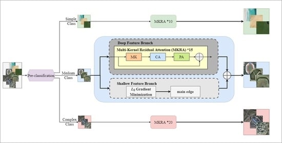
In this section, we describe the overall architecture and specific details of our method, including the preclassification strategy, the network design, and the loss functions. To have a better understanding of our work, we first give a brief introduction to the method. The overall scheme is shown in
Figure 1. According to the structural complexity of the input remote sensing images, different SR networks are designed to reconstruct the corresponding remote sensing images, reducing the training samples and difficulty of each network.
3.1. Preclassification Strategy
Remote sensing images contain a variety of scene types, e.g., mountain, forest, city, ocean, desert, etc., whose scene structure complexity is very different. Existing SR networks process all kinds of remote sensing images without distinction, resulting in large training samples and difficulty to obtain excellent reconstruction results. In this paper, the idea of preclassification is innovatively highlighted. The datasets and networks are classified according to the different complexity of remote sensing images, to reduce the number of training samples and improve the effect of the SR network.
Since the complexity of remote sensing images is mainly reflected in image details such as edges, the average image gradients are used to measure the image complexity in this paper. With simplicity in mind, remote sensing images are divided into three classes according to their complexity, namely, the simple class, the medium class, and the complex class. Examples of each class and their gradient images are shown in
Figure 2. Images in the simple class mostly contain monotonous and regular geographical areas, while images in the complex class contain a variety of ground objects. Remote sensing images of different complexity are designed to be processed by different networks, and the difference of networks is mainly reflected in the number of sub-modules, which does not increase the design complexity. Each network learns the commonality of the remote sensing images in each class, which gives the network good capability of reconstructing the congeneric images and reduces the overall training difficulty as well.
3.2. Deep–Shallow Features Fusion Network
Remote sensing images usually have the problem of weak edge details. When extracting image features, the deep network tends to weaken the shallow features, such as edges and contours, so we propose an SR network based on the fusion of deep and shallow features. Our network architecture is mainly divided into a deep feature branch and a shallow feature branch, as shown in
Figure 3. The deep feature branch is used to extract deep features of remote sensing images, and the shallow feature branch integrates the shallow features of remote sensing images into the end of the network. The deep features and the shallow features are fused to generate the HR image.
Since the input image and the target image are highly correlated in the SR task, the global residual learning is adopted in the network, to reduce the complexity and learning difficulty of the network. To effectively extract the deep features of LR, we design the multi-kernel residual attention (MKRA) module. In general, when a network has deep layers, it can learn more complex representations, but it brings the increase of parameters number. Networks are built by controlling the number of MKRA and convolution filters to adapt to the different remote sensing images. Meanwhile, in view of the characteristics of weak edges in remote sensing images, we extract the main edge of LR images as shallow features to supervise the network to produce details. Specifically, the branch of shallow feature first smooths the image with
gradient minimization [
23] to reduce noise and secondary information, then extracts the edge and fuses it into the end reconstruction part to improve the edge reconstruction effects.
In a word, the deep feature branch consists of convolution layers, multiple MKRA modules, and upsample parts. The shallow feature branch consists of an
gradient minimization, a convolution layer, and an upsample part. Inspired by EDSR [
18], sub-pixel convolution [
16] is the upsampling part in the network.
3.2.1. Multi-Kernel Residual Attention
For neural networks, higher-level feature extraction and data representation are all crucial [
24]. Similarly, for the SR tasks of remote sensing images, stronger characterization ability is conducive to achieving better performance. The size of convolution kernel determines the way of feature extraction, so we adopt multi-kernel convolution for feature extraction to improve the richness of feature. Moreover, local residual connection and attention mechanism are adopted to further optimize the feature utilization capacity of the network. Each MKRA module shown in
Figure 4 is composed of multi-kernel (MK) convolution sub-module, channel attention (CA) sub-module, and pixel attention (PA) sub-module.
Figure 5 demonstrates the detail of sub-module in MKRA. The feature maps are fused and activated by nonlinear function after four convolution kernels of different sizes (3 × 3, 1 × 3, 3 × 1, 1 × 1). To avoid size mismatches in the training process, the zero-padding approach is adopted to ensure the image size remains consistent during feature delivery. The local residual connection in the modules is beneficial to avoid the training instability and generalization ability caused by the deeper network.
Early CNN-based SR methods mainly focused on increasing the depth and width of the network, while features extracted from the network were treated equally in all channels and spatial regions. These methods lack the necessary flexibility for different feature mapping networks and waste computational resources in the task. The attention mechanism enables the network to pay more attention to the information features that are more useful to the target task, and suppress the useless features, so that the computing resources can be allocated more scientifically in the feature extraction process, to deepen the network effectively [
25,
26,
27]. We use the cascade of channel attention and pixel attention to enhance the features and improve the learning ability of modules.
Figure 5 and
Table 1 report the MK, CA, PA design structure, and data flow in more detail.
3.2.2. Shallow Features Extraction
Deep CNNs with numerous convolution layers are hierarchical models and naturally give multilevel representations of input images, the lower layer representations focus on local details (e.g., edge and contours of an object) and the higher layer representations involve more global priority (e.g., environmental type). It also brings limitations that there are only high-dimensional deep features left, while the edge, texture, contour, and other shallow features of the image disappear at the end of the network.
Therefore, we extract the edge details of the original LR image and perform complementary fusion at the end of the network. However, for remote sensing images with complex scene structure, the main edge information is mixed with the secondary edge information, and the secondary information interferes with the neural network model to a certain extent. As a result, we use
gradient minimization [
23] to filter out the secondary edge information in the concrete implementation, and the gradient of the new image is more conducive to the recovery of main edge image information. The image differences with or without
gradient minimization are shown in
Figure 6. Note that images with
gradient minimization maintain the main edge to the maximum extent and can effectively supplement the shallow feature deficiency caused by the deep network.
3.3. Loss Function
Our networks are trained by supervised learning, and the loss function is the ultimate goal of the network, which is very important to guide the training process of the network [
28]. In light of the characteristics of remote sensing images, edge loss and cycle consistent loss [
29] based on charbonnier loss [
24] are added to make network convergence faster and easier. As usual, the loss function first calculates the holistic and detailed differences between HR image and SR image to guide the gradient optimization process of the network. The charbonnier loss calculates the overall difference between SR image and HR image:
where
denotes the HR image and
denotes the SR image, and the constant
is empirically set to
for all the experiments.
To make full utilization of edge information, we apply edge loss to calculate the edge difference between HR images and SR images, to improve the effect of reconstruction of texture details such as edges. The calculation formula for edge loss is as follows:
where
denotes Laplacian operator.
In addition, SR is an inherently ill-posed problem where many more HR pixels need to be estimated under limited known LR pixels, which is where an LR may have multiple HR pairs. If we only focus on learning the mapping from LR images to HR images, the space of possible mapping functions may be very large, which makes training very difficult. The process from LR images to SR images is seen as positive and the process from SR images to LR images is seen as reversed, which can form a cycle. Obviously, downsampled
should be consistent with
, so we use cycle consistent loss to make better utilization of
and narrow the range of SR solutions. In other words, we not only pay attention to the proximity of
and
, but also pay attention to the proximity of
and
after downsampling. The calculation formula for cycle consistent loss is as follows:
where
represents the SR image downsampled by bicubic to the same resolution as
.
In the end,the total loss function can be expressed as
where
and
are used to adjust the weights of edge loss and cycle consistent loss.
As the same form of loss calculation is adopted, the calculation value is in the same order of magnitude, so we set and to 1, avoiding the difficulty of hyperparameters setting.
4. Experiment
In this section, we first introduce two remote sensing datasets and the implementation details of our SR networks. After that, we perform experiments to verify the effectiveness of preclassification strategy. Finally, we fully compare our method with various state-of-the-art methods, and display quantitative evaluation and visual comparison.
4.1. Dataset Settings
We choose two datasets with plentiful scenes to verify the robustness of our proposed method. There are some training images shown in
Figure 7.
WHURS [
30]: This is a classical remote sensing dataset, which consists of 1005 images in 19 classes of remote sensing images with different geographical topography, including airport, beach, bridge, commercial, etc. All images are in
pixels and the spatial resolution is up to 0.5 m/pixel. We randomly select 10 images from each class as the testing set, and the rest as the training set.
AID [
31]: This is a large-scale aerial image dataset that collects sample images from Google Earth images. The AID dataset contains 10,000 images of 30 land-use scenes, including river, mountain, farmland, pond, and so on. All sample images of each category were carefully selected from different countries and regions of the world and extracted at different times and seasons under different imaging conditions, which increases the diversity in the classes of the data. We randomly select 20% of the total number as the testing set, and the remaining 80% as the training set.
4.2. Implementation Details
We design corresponding networks for remote sensing images of different complexity, and the main framework of these networks is similar, as shown in
Figure 3. The three corresponding sub-networks (simple net, medium net, complex net) in
Figure 1 are established by controlling the number of MKRA and the number of convolutional channels. To save memory and reduce computation, simple net has 10 MKRAs with 32 channels, medium net has 15 MKRAs with 48 channels, and complex net has 20 MKRAs with 64 channels.
Following the settings of EDSR [
18], in each training batch, the input LR images are randomly cropped in a patch size of
, and the corresponding input HR images with sizes of
,
, and
are cropped according to the upscaling factors
,
, and
, respectively. To produce the LR input frames, we downsample the HR frames through bicubic [
32] interpolation. In addition, the training sets are also augmented via three image-processing methods: horizontal flipping, vertical flipping, and 90 rotation. More detailed parameter settings are indicated in
Table 2. The proposed algorithm is implemented under the PyTorch [
33] framework on a computer with an NVIDIA GTX 2080Ti GPU.
4.3. Preclassification Experiment
To verify the effectiveness of the preclassification strategy, we first use the classical SR network EDSR to conduct validation experiments on scales
,
, and
. As shown in
Table 3, with the preclassification strategy, the remote sensing images with different complexity have been improved, especially the remote sensing images with higher complexity. The preclassification strategy has strong transferability and universal applicability, especially for various remote sensing images.
4.4. Quantitative and Qualitative Evaluation
In this section, the proposed method is evaluated with other methods quantitatively and qualitatively. To further verify the advancement and effectiveness of the proposed method, we compare our method with bicubic [
32] and five other state-of-the-art methods: very deep super-resolution (VDSR) [
15], enhanced deep super-resolution (EDSR) [
18], pixel attention network (PAN) [
19], local–global combined network (LGCNet) [
21], and deep residual squeeze and excitation network (DRSEN) [
22]. Bicubic interpolation is a representative interpolation algorithm. VDSR adopts residual learning to build a deep network. PAN builds a lightweight CNN with pixel attention for quick SR. EDSR is a representative version of deep network architectures with residual blocks. LGCNet and DRSEN are two SR methods for remote sensing images. To fairly compare the performance of the networks, the number of residual blocks for EDSR and the number of RSEB for DRSEN are set to 20, and both convolution filters are all set to 64. For a fair comparison, these methods are retrained under our training datasets.
The model size is a critical issue in practical applications, especially in devices with low computing power. Furthermore, for the scale factor
,
Figure 8 illustrates the comparison of the number of parameters between our SR network and other networks. Our simple net is close to the network with the minimum number of parameters, while the parameters number of complex net is less than EDSR and DRSEN. This provides an appropriate network for applications in different scenarios.
4.4.1. Quantitative Evaluation
We adopt the peak signal-to-noise ratio (PSNR) [
35] and structural similarity (SSIM) [
36] as the objective evaluation indexes to measure the quality of the SR image reconstruction. The PSNR is one of the most widely used standards for evaluating image quality, and it compares the pixel differences between HR and SR images. Larger PSNR values indicate lower distortion and a better SR reconstruction effect. The SSIM is another widely used measurement index in SR image reconstruction, which is based on the luminance, contrast, and structure of HR image and LR image. If the SSIM value is closer to 1, then the similarity is greater between the SR image and the HR image, a.k.a., the higher the quality of the SR image.
It can be seen from the experimental results that the amount of training data of a single network is reduced to about 1/3 of the original dataset by the preclassification strategy proposed in this paper, but the reconstruction effect is greatly improved. Compared with other SOTA methods, our method achieves the best results in both PSNR and SSIM with different scale factors, and can adapt to the SR requirements of different scales. In addition,
Table 4 implies the mean results of each method on WHURS and AID datasets with
,
, and
scale factors, which reveals that our model outperforms other methods. On the WHURS testing set with scales
,
, and
, the PSNR and SSIM of our method reach 36.4095/0.9512, 31.8460/0.8701, and 29.4892/0.7976, respectively. It outperforms the second-best model, DRSEN, with PSNR gains of 0.1289 dB, 0.1954 dB, and 0.1428 dB, with SSIM gains of 0.0010, 0.0036, and 0.0104. The comparison results of PSNR and SSIM are more visually depicted in
Figure 9. In particular, SSIM values under large scale (
) are increased by 0.0104 and 0.0114 in WHURS and AID testing sets, respectively, equivalent to 1.32% and 1.49% higher than DRSEN (second place method), indicating that our method can effectively reconstruct the structural information of remote sensing images.
4.4.2. Qualitative Evaluation
To more fully illustrate the effectiveness of our method, the reconstruction results are examined qualitatively and some of the visual comparisons are demonstrated in
Figure 10. It is noteworthy that our method achieves better results on the different scenes, reducing sawtooth and better reconstructing the structure and edge of the objects in the images. On the basis of numerical analysis in
Table 5, we can find that large diversity exists among these remote sensing image classes, showing the authenticity and diversity of the test datasets. As can be seen from the visual results in
Figure 10, compared with various typical deep learning SR methods, the proposed method in this paper has clearer details of reconstructed grain edges and richer details and textures. For a clearer comparison, a small patch marked by a red rectangle is enlarged and shown for each SR method.
The bicubic upsampling strategy results in loss of texture and blurry structure, which is more obvious for remote sensing images with weak edge details. VDSR and LGCNet take such bicubic upsampling results as network inputs, and then they produce erroneous structural and texture information and fail to recover more details, ultimately resulting in poor SR image quality. Other methods directly use LR as input, then achieve better results, but they do not take into account the characteristics of remote sensing images; the edges are still difficult to distinguish, as shown in
Figure 10a. The results of our method have more clearly differentiated edges, which also can suppress noise and maintain the color consistency of local regions, as depicted in
Figure 10c, while being closer to high-resolution images.
4.5. Discussion
According to the quantitative and qualitative evaluation in
Section 4.4, the proposed method performs better than the other methods. Our method can be used as a reference solution for the problems such as the diversity of remote sensing images and the weakening of edge details. However, there are some limitations.
On the one hand, a mass of paired higher-quality images is necessary for deep learning, but it is often difficult to obtain pairs of high-resolution and degraded images. When training the network, we use bicubic method to produce the corresponding low-resolution images from high-resolution remote sensing images. However, in actual situations, the bicubic method does not fully represent the degradation process of remote sensing images. Our method may be inadequate for some extremely distorted images. The degradation process of remote sensing images needs further study in the future.
On the other hand, although some images at the intersection of intervals can be classified according to the proposed preclassification strategy, compared with the image inside the interval, this strategy is too simple and direct, so the classification based on fuzzy ideas can be explored in the future method.
5. Conclusions
In view of the characteristics of remote sensing images, we propose an SR method for remote sensing images using preclassification strategy and deep–shallow features fusion. The preclassification strategy divides remote sensing images into three classes according to the structural complexity of scenes, and different networks are applied for each class. In this way, the training difficulty of each network is reduced, and each network can learn the commonness of same-class images. Moreover, considering the weak edge structure of remote sensing images, our networks are shallow features fused to deep features.We smooth the LR images by gradient minimization, and extract the main edge of the new LR images as the shallow features. The MKRA module is proposed to extract deep features, and the shallow features are integrated at the end of the deep network. Finally, the edge loss is added to improve the edge reconstruction effect and the cycle consistent loss is added to raise utilization of LR images. Numerous comparative experiments demonstrate that the SR method in this paper can enrich texture details of reconstructed images and provide better visual effects, and the PSNR and SSIM values of quantitative parameters are also generally improved. More advanced classification methods will be considered in the future to further reduce the number of training samples required, as well as the degradation process of different scenarios.


 ,
, 


