Monitoring the Hydrological Activities of Antarctic Subglacial Lakes Using CryoSat-2 and ICESat-2 Altimetry Data

Abstract

Monitoring the hydrological activities of subglacial lakes is critical to understanding the subglacial hydrological system and evaluating the internal mass changes of the Antarctic ice sheet. Drainage or filling events of active lakes lead to elevation changes in the ice surface. These changes can be observed by satellite altimetry, but the monitoring must be conducted continuously since the water movements in active subglacial lakes may occur frequently. We used CryoSat-2 Baseline-D and ICESat-2 data from 2010 to 2020 to obtain the time series of the ice surface elevation changes for 17 active lakes. We also evaluated the uncertainty of the time series derived from the CryoSat-2 data by cross-validation. The mean and RMS of the biases between the CryoSat-2-based and ICESat-2-based time series are generally less than 0.3 m and 1.0 m, respectively. However, the mean and RMS are greater over the lakes with rough ice surfaces, such as Whillans₆, KT1, Mac3, and Slessor₂₃. The drainage and filling events continue exhibiting in the extended period and the hydrological activities of SLW, L12, Whillans₆, L78, and Mac1 occurred periodically. Furthermore, we inferred the hydrological connections between the lakes combining simulated water pathways.

1. Introduction

Subglacial lakes have long been considered independent and relatively steady, closed water bodies beneath the Antarctic ice sheet (AIS) [1]. With the development of satellite altimetry and satellite radar interferometry techniques, massive numbers of satellite measurements were obtained in chronological order in the ice sheet. Previous studies used satellite data to map ice surface elevation anomalies in regions with active subglacial lakes, which are believed to be caused by the filling and draining of subglacial water [2,3,4]. Based on this knowledge, numerous active subglacial lakes have been identified in fast-moving ice streams or glaciers at the edge of the ice sheet using satellite altimetry data [5,6]. These subglacial lakes transferred water to other adjacent lakes when episodic drainage events occurred, causing regional uplifts and collapses of the ice surface. The loss of water and ice due to the rapid movement of water from upstream to downstream can alter the Antarctic mass balance [3,7]. Therefore, investigating the hydrological activities of active subglacial lakes is crucial for accurately evaluating the mass balance of the AIS.

Satellite altimetry can provide long-term ice surface elevation data and has significant advantages, including wide coverage and high accuracy. It is not only used to identify active subglacial lakes, but also has become an important means to monitor their activities [7,8,9,10]. NASA’s Ice, Cloud, and land Elevation Satellite (ICESat) provides elevation data with high accuracy, small footprints ($~$70 m), and dense along-track sampling. Due to the unique design of the two receiving antennas of the European Space Agency’s CryoSat-2 in the Synthetic Aperture Radar Interferometric (SARIn) mode [11], CryoSat-2 measurements possess high enough accuracy even in areas with complex topography around the ice sheet margins. Therefore, ICESat and CryoSat-2 SARIn data have become primary data sources for studying the activities of subglacial lakes [12,13,14,15,16,17]. In the studies mentioned above, Fricker et al. (2007) [4] used repeat-track analysis to process ICESat data from 2003 to 2006 and found that the subglacial lakes beneath the Mercer, Whillans, and MacAyeal Ice Streams were linked, forming a subglacial hydrological system. Siegfried et al. (2014) [12] combined ICESat and CryoSat-2 SARIn data and found that the subglacial lake activities occurred frequently beneath the Mercer and Whillans Ice Streams. A similar story played out at another active glacier in Antarctica. Based on CryoSat-2 SARIn data, Smith et al. (2017) [15] identified four connected subglacial lakes under the Thwaites Glacier which experienced large-scale drainage events between June 2013 and January 2014. Only 4 years later, large-scale subglacial water activities occurred again in these lakes [17]. The frequent transports and exchanges of water in active subglacial lakes prove the importance of monitoring hydrological activities in a more timely and precise manner. Siegfried and Fricker (2021) [18] used CryoSat-2 and ICESat-2 data to extend the activity time series of five lakes in CryoSat-2 SARIn mode to 2020. In addition to the five lakes, and the four lakes under the Thwaites Glacier [17], the time series of the other lakes in the SARIn mode were only extended to 2016 [16].

In this study, we refine the time series of the ice surface elevation changes of 17 most representative active subglacial lakes in Antarctica and extend to 2020 using CryoSat-2 Baseline-D and ICESat-2 data. ICESat-2 has the overlapping mission periods with CryoSat-2 and is used to validate the time series obtained from the CryoSat-2 data. We then define the periodicity of the hydrological activities of the subglacial lakes and discuss the hydrological connections between the subglacial lakes in the same basins, combining the temporal and spatial evolution of the ice surface elevation changes with simulated subglacial water pathways.

2. Data

2.1. CryoSat-2

CryoSat-2 was launched in April 2010 and has a 369-day repeat cycle, including a subcycle of 30 days. It operates in three data collection modes. CryoSat-2 measures the interior of the AIS using the Low Resolution Mode (LRM) and the margins of the ice sheet using the SARIn mode. The Synthetic Aperture Radar (SAR) mode is used for sea ice.

Due to the use of two receiving antennas operating in an interferometric mode, SARIn is very suitable for precisely measuring the rough surface at the ice sheet margins, where most active subglacial lakes exist. CryoSat-2 Level 2 (L2) Baseline-D ice products released in 2019 can provide better results for land ice than the Baseline-C products used in previous studies, improving the ascending and descending crossover statistics from 1.9 to 0.1 m [19], substantially reducing the impact of track deviation on the estimation of ice surface elevation changes [20]. We used CryoSat-2 L2 Baseline-D data in the SARIn mode from July 2010 to October 2020 to calculate the ice surface elevation changes.

2.2. ICESat-2

ICESat-2 was launched in September 2018. As the follow-on satellite of ICESat, ICESat-2 continues to provide measurements of polar sea ice and ice sheet elevation. ICESat-2 is equipped with the Advanced Topography Laser Altimeter System (ATLAS) and collects data up to $\pm$88° latitude in a 91-day repeat cycle with a subcycle of 30 days [21]. Compared with the first generation, ICESat-2 has a smaller footprint ($~$17 m), higher resolution for along-track sampling, higher density for across-track sampling, and higher accuracy and reliability of ground observations. Brunt et al. (2019) [22] used Global Navigation Satellite System (GNSS) data to validate ICESat-2 ATL06 data and showed that the accuracy and precision of ICESat-2 ATL06 data was less than 0.03 m and 0.09 m, respectively. We calculated the ice surface elevation changes and validated the results obtained from the CryoSat-2 data using ICESat-2 ATL06 data from October 2018 to October 2020.

2.3. REMA

The Reference Elevation Model of Antarctica (REMA) is a high-resolution digital ice surface elevation model released by the Polar Geospatial Center (PGC) of the United States. It covers land ice areas ranging from 60°S to 88°S with 8 m spatial resolution [23]. In addition to a data set with 8 m resolution, PGC also provides resampled versions with 100 m, 200 m, and 1 km resolutions. We used the REMA product with 100 m resolution as the reference surface for calculating elevation anomalies.

3. Methods

We collected the outlines of 17 active subglacial lakes beneath four ice streams and one glacier in Antarctica [5,7,8,14,16]; 9 lakes (L10, L12, L78, SLC, SLE, SLM, SLW, USLC, and Whillans₆) were beneath the Mercer and Whillans Ice Streams, 3 lakes (KT1, KT2, and KT3) were beneath the Kamb Ice Stream, 3 lakes (Mac1, Mac2, and Mac3) were beneath the MacAyeal Ice Stream, and 2 lakes (Slessor₁ and Slessor₂₃) were beneath the Slessor Glacier.

3.1. Creation of CryoSat-2-Based Elevation Change Time Series

3.1.1. Data Preprocessing

In this study, we developed a method to filter the outliers in the CryoSat-2 SARIn data. We first removed the outliers outside of the actual elevation range of the AIS due to instrument failures, abnormal equipment signals, and incorrect processing. We then divided the data of each lake according to the track numbers and removed the data deviating from the center of the ground track by fitting the data of each track. Next, we used a time step of 3 months centered every month [12] from August 2010 to September 2020 to divide the data into subsets over the lakes. We divided each subset into corresponding grids according to the ground positions and fitted each grid’s data using least squares surface fitting. Data with elevation residuals greater than the threshold were removed. The remaining data were continuously fitted and filtered until no data with elevation residual exceeding the threshold remained or the number of the remaining data in the grid was less than the minimum number required for fitting. After carrying out experiments and considering the data characteristics, we used 10 km $\times$ 10 km grids and 3 times the standard deviation of the elevation residuals at each grid as the threshold.

3.1.2. Creation of Elevation Change Time Series

For this step, we generally followed the methods described in recent studies [12,13,16,18]. We subtracted the REMA elevations interpolated at the footprint locations from the filtered data subsets within the 3-month interval to calculate elevation anomalies. We then calculated the mean elevation anomaly within the outline of each subglacial lake. In addition to the subglacial water movement, the mean elevation anomaly contained the contribution from the regional elevation change related to snowfall, snow compaction, wind-induced snowdrift, and ice flow [24]. We built a buffer zone extending 5 km from the outline and calculated the mean elevation anomaly in the buffer zone to estimate regional elevation change. We calculated the difference between the mean elevation anomalies within the outline and the buffer zone to obtain the monthly time series of the ice surface elevation changes caused by the lake activities. In this step, the regional elevation changes within the outline and the buffer zone were assumed to be equal [12].

3.2. Creation of ICESat-2-Based Elevation Change Time Series

The ICESat-2 ATL06 data were labeled with standard quality flags. We removed the erroneous elevation records according to the provided quality flags and obtained the time series of the ice surface elevation changes caused by subglacial lake activities from November 2018 to September 2020 using the methods described in Section 3.1.2.

3.3. Hydraulic Potential and Simulation of Subglacial Water Pathways

The flow and storage of subglacial water under the ice sheet is mainly governed by gradients in the hydraulic potential, which is a function of ice surface elevation and bedrock elevation [25]. The hydraulic potential beneath the ice sheet is calculated as follows:

$${\varphi }^{\prime }={\rho }_{i}g{z}_s+\left({\rho }_{w}g-{\rho }_{i}g\right)z_b$$

(1)

where ${\varphi }^{\prime }$ is the hydraulic potential in units of pressure, ${\rho }_i$ and ${\rho }_w$ are the densities of ice (917 kg/m³) and fresh water (1000 kg/m³), $z_s$ and $z_b$ are the ice surface and bedrock elevation with respect to the geoid, and $g$ is the gravitational acceleration. The hydraulic potential in units of elevation is obtained by dividing ${\varphi }^{\prime }$ by the unit weight of fresh water:

$$\varphi =\frac{{\varphi }^{\prime }}{{\rho }_{w}g}=\frac{{\rho }_i}{{\rho }_w}{z}_s+\frac{{\rho }_w-{\rho }_i}{{\rho }_w}{z}_b$$

(2)

We used the ice surface and bedrock elevation data from the Bedmap2 dataset [26] to map a hydraulic potential surface with a resolution of 1 km. In this step, we filled locally closed depressions within the basins to generate a potential surface through which subglacial water can steadily flow [15] and simulated the possible subglacial water pathways over the potential surface using the Hydrology Analyst Tools in the ArcGIS package.

4. Results

4.1. Cross-Validation

CryoSat-2 and ICESat-2 had overlapping missions from October 2018 to October 2020, and ICESat-2 provides observations with higher accuracy and denser coverage than CryoSat-2. We calculated the biases between the CryoSat-2-based time series of the ice surface elevation changes and the ICESat-2-based time series month by month. The mean and RMS of the biases between the two time series over each lake are given in

Table 1. Statistics of the biases between the CryoSat-2-based and ICESat-2-based time series.

Basin	Lake	Mean (m)	RMS (m)
Mercer and Whillans Ice Streams	L10	0.04	0.17
	L12	0.14	0.65
	L78	−0.14	0.65
	SLC	−0.13	0.60
	SLE	0.05	0.23
	SLM	−0.13	0.64
	SLW	0.17	0.79
	USLC	0.18	0.87
	Whillans6	−0.35	1.67
Kamb Ice Stream	KT1	−0.34	1.56
	KT2	0.03	0.14
	KT3	0.01	0.05
MacAyeal Ice Stream	Mac1	−0.16	0.77
	Mac2	−0.21	0.99
	Mac3	−0.25	1.18
Slessor Glacier	Slessor1	−0.07	0.32
	Slessor23	0.70	3.34

. In most lake regions, the mean biases between the two time series are less than 0.3 m, and the RMS are less than 1.0 m. The mean and RMS of the biases are greater at Whillans₆, KT1, Mac3, and Slessor₂₃. Among them, the mean and RMS are 0.70 m and 3.34 m over Slessor₂₃.

Different from ICESat-2, CryoSat-2 SARIn data points are not distributed along repeat-tracks because SARIn mode tracks the points of topographic highs. The differences in the accuracy and distribution of the data led to the biases between the two time series. The locations of the subglacial lakes are shown in Figure 1. It can be seen that the ice surfaces are rough in the regions of Whillans₆, KT1, Mac3, and Slessor₂₃. The slope and roughness of the ice surfaces of the four lakes led to greater biases between the two time series than other lakes. In addition, the areas of Whillans₆ and KT1 are very small (71 km² and 44 km², respectively), and Mac3 is a long and narrow lake. These pose great challenges to our work.

In order to present the difference of the data distribution more intuitively, we show the ICESat-2 and CryoSat-2 elevations from 2018 to 2020 at Slessor₂₃ in Figure 2. The ice surface of Slessor23 is steep, and there are few CryoSat-2 data on the low surface west and southwest of the lake, whereas the ICESat-2 data are dense. Therefore, the biases between the two time series are great over Slessor₂₃.

In summary, the CryoSat-2-based time series values are in general agreement with the ICESat-2-based time series values in flat lake regions, and the mean and RMS of the biases between the two time series are greater over the lakes where the ice surfaces are rough such as Whillans₆, KT1, Mac3, and Slessor₂₃.

4.2. Time Series of the Ice Surface Elevation Changes

The obtained time series show similar elevation changes in the ice surfaces of the subglacial lakes with those in previous studies [16,18]. We focused our analysis on the extended time series from November 2016 for 12 lakes and July 2020 for five lakes and overall analyzed the decade time series to give suggestions on the periodicity of the hydrological activities in the lakes. However, the amplitude differences of the time series in different studies should be noted, as a result of improved data and processing.

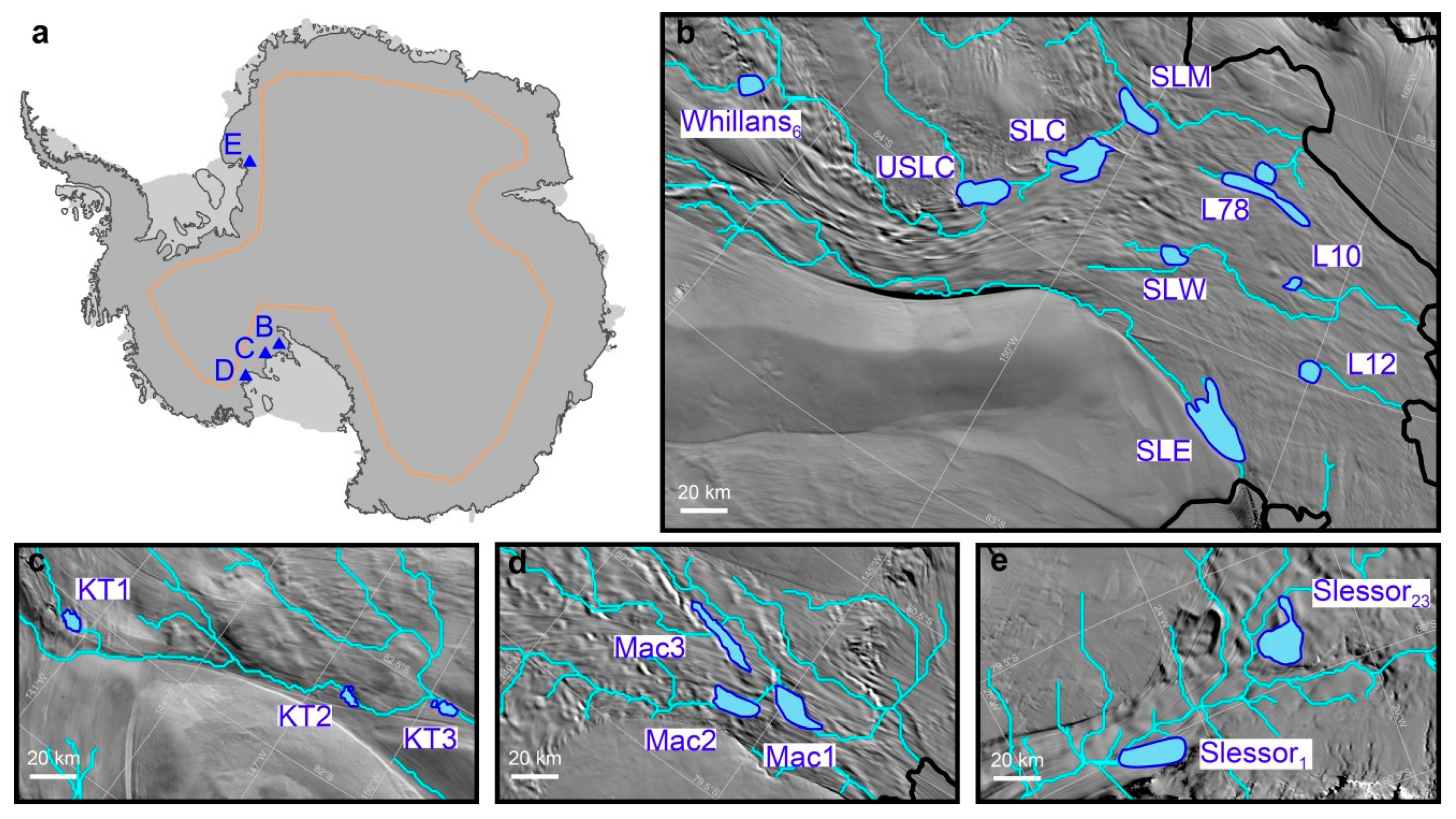
4.2.1. Mercer and Whillans Ice Streams

The Mercer and Whillans Ice Streams are hot areas for studying the active subglacial lakes in Antarctica. We obtained the time series of the ice surface elevation changes of nine active subglacial lakes in the areas (Figure 1b). Our results are shown in Figure 3.

In the extended period, the ice surface elevation of SLE continued to increase at the rates of 0.1–0.2 m/year, while that of L10 decreased at the rate of −0.1 m/year (Figure 3). From late 2016 to early 2020, the ice surface elevation increased at the rate of 0.1 m/year at SLW, while it slowly decreased at L12. The ice surfaces of SLW and L12 rapidly increased by 1.7 m and 1.2 m, respectively, over the next few months. The ice surface elevation of Whillans₆ increased by 1.7 m and decreased by 2.1 m during the fill–drain cycle (one fill event and one drain event were defined as one fill–drain cycle) from mid-2017 to 2020.

The ice surface elevation at USLC started to increase in mid-2017 and peaked in early 2018 after increasing by 2.6 m and subsequently remained near the peak. In the regions of SLC and SLM, we extended the time series by only 2 months compared to the mentioned study [18]. Over the 2 months, the ice surfaces of the two lakes were stable.

From mid-2017, two fill–drain cycles occurred at L78. The mean elevation change of the ice surface was very small ($<$1 m) during the cycles, and there was almost no interval between the two cycles.

As mentioned above, the extended time series show the hydrological activities in the subglacial lakes, and they occurred periodically in SLW, L12, Whillans₆, and L78. During the CryoSat-2 mission, SLW and L12 experienced two fill–drain cycles and were likely to enter the third cycle. The period between the last two cycles (about 4 years; 2016–2020) was longer than that between the first two cycles (about 3 years; 2013–2016), indicating that the melting of the ice nearby SLW and L12 slowed down and the subglacial water discharge upstream reduced. Not only that, SLW also experienced two fill–drain cycles in the ICESat period [16], with the periods of about 2 years (2006–2008) and 5 years (2008–2013), while L12 exhibited only a cycle due to the lack of ICESat data. Based on these findings, we believed SLW and L12 experienced periodic hydrological activities with a period of 2–5 years. At Whillans₆, the two fill–drain cycles occurred within 1.5–3 years, with a period of about 2.5 years.

L78 was the most especial lake in the areas. In the four fill–drain cycles, the periods between the first two cycles and between the last two cycles were much shorter than the period between the second and third cycles. It is reasonable to combine the first two cycles into a main-cycle (so-called to distinguish it) and the last two cycles into the second main-cycle. The peak (1.7 m in 2012) of the first main-cycle was higher than that (near 1 m in 2020) of the second, and the period between the two main-cycles was about 6 years (2012–2018). In addition, we noted that L78 experienced another main-cycle (see Figure 2 of Siegfried and Fricker, 2018 [16]), and the period was also about 6 years (from late 2005 to 2012). These records indicated that L78 might have a constant period of about 6 years combined successive cycles into main-cycles.

4.2.2. Kamb Ice Stream

Figure 4 shows the time series of the ice surface elevation changes of the subglacial lakes KT1, KT2, and KT3 (Figure 1c) beneath the Kamb Ice Stream. In the extended time series, KT1 was the only lake with the elevation changes in the ice surface. However, the elevation changes might be overestimated due to the rough ice surface in the KT1 region as mentioned in Section 4.1.

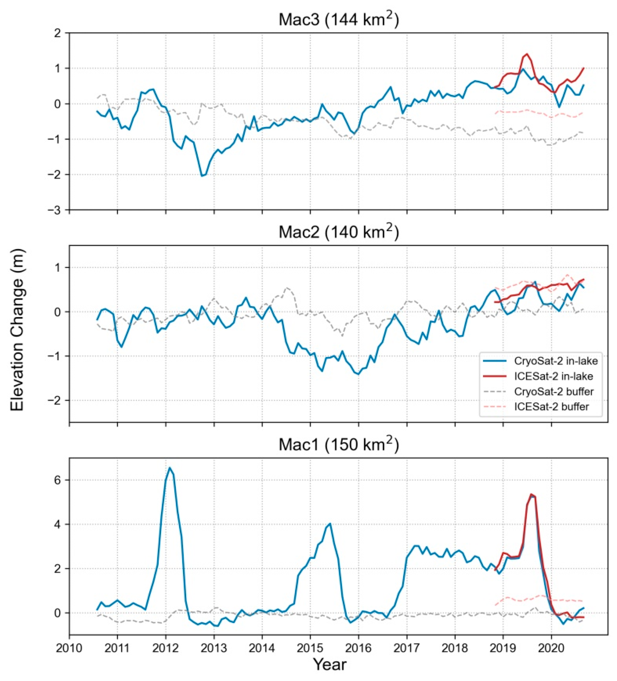
4.2.3. MacAyeal Ice Stream

We analyzed the subglacial lakes Mac1, Mac2, and Mac3 (Figure 1d) on the lower MacAyeal Ice Stream. Our results are shown in Figure 5. The time series of the three lakes (extended to 2020) were given in Siegfried and Fricker (2021) [18]. It should be noted that there were the amplitude differences between the time series in this study and those in the previous study. We believed that the improved data processing and different areas of the buffer zones led to the differences. In this study, the CryoSat-2-based time series values were more agreement with the ICESat-2-based time series values over Mac2, with the mean bias and RMS of −0.21 m and 0.99 m.

As shown in Figure 5, Mac1 experienced three fill–drain cycles. The peaks in the three cycles were different, and the mean ice surface elevation at Mac1 never returned the highest level (6.5 m in 2012), indicating the storage limits of the lake were always changing. The first two fill–drain cycles occurred within 1.5 years, and the third cycle started only about half a year later. The shorter interval indicated that the ice melting accelerated in the ice stream. It can be seen that the discharge of the water upstream suspended in 2017–2019, and the third fill–drain cycle of Mac1 lasted much longer than other cycles. The peaks show that Mac1 had a period of 3.5–4 years (2012–2015 and 2015–2019; 2004–2008 and 2008–2012, see also in Figure 4 of Siegfried and Fricker 2018 [16]).

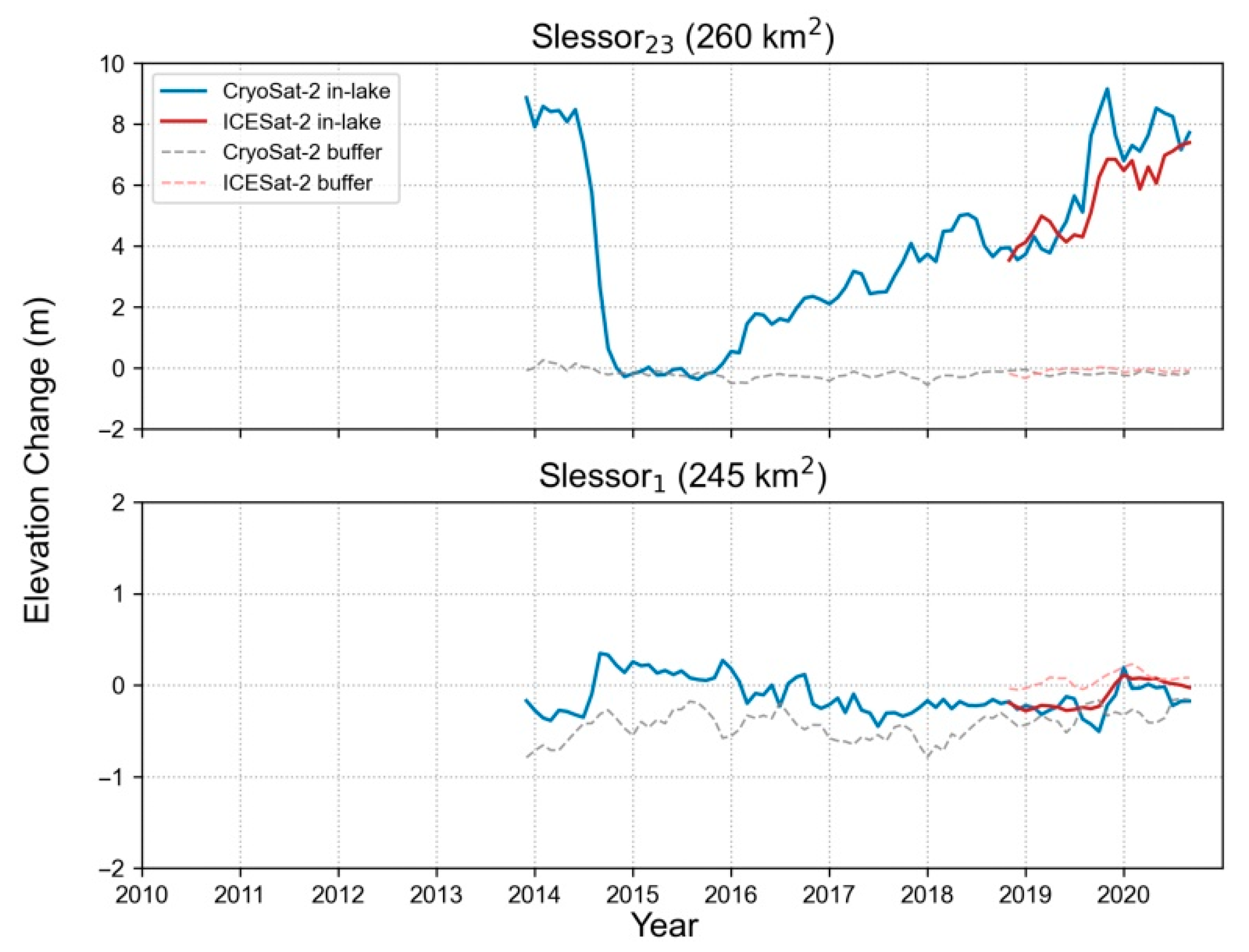
4.2.4. Slessor Glacier

The subglacial lakes Slessor₁ and Slessor₂₃ (Figure 1e) beneath the Slessor Glacier were covered by CryoSat-2 SARIn mode after October 2013, when the mission was adjusted. The time series of the ice surface elevation changes are shown in Figure 6. In the extended time series, the ice surface elevation at Slessor₂₃ rapidly increased by 5.4 m in 7 months in 2019 and reached a high level of 9.2 m (might be overestimated). The ice surface over Slessor₁ was stable from 2017 to late 2019 and then increased by 0.7 m (this value was smaller in the ICESat-2-based time series).

We comprehensively monitored the long-lasting hydrological activity of Slessor₂₃ by extending the time series to the present. Slessor₂₃’s filling period lasted for up to 4 years (2015–2019) after the large-scale drainage. In other words, Slessor₂₃ experienced a drain–fill cycle of 5.6 years (2014–2019), which occurred during the whole CryoSat-2 mission. The water level of Slessor₂₃ returned to a high level, and the next large-scale drainage was likely to occur in the near future at the time of writing.

5. Discussion

5.1. Hydrological Analysis

Calculating the hydraulic potential beneath the ice sheet for simulating the subglacial water pathways is a common method to show where the water can travel from the subglacial lake when the drainage event occurs [6,7,10,14,15,29]. We followed previous studies and interpreted the elevation change in the ice surface of the subglacial lake as the water level change, although the surface change might be delayed due to the viscosity of ice layer.

Figure 1d shows that Mac1 and Mac2, as well as Mac1 and Mac3, were hydrologically linked. Siegfried and Fricker (2021) [18] inferred that Mac1 had a water source in addition to Mac2 and Mac3 because the amount of the water travelled to Mac1 was much greater than those discharged from Mac2 and Mac3. We inferred that the third water pathway linked the water source with Mac1.

The subglacial water pathways linked Slessor₂₃ with Slessor₁ and skirted the main body of Slessor₁ (Figure 1e), indicating that the hydrological connection between the two lakes might be weak. As shown in Figure 6, the large-scale drainage event of Slessor₂₃ in 2014 had a small impact on the water level of Slessor₁, and the rapidly increasing of the water level of Slessor₂₃ in 2019 coincided with that of Slessor₁, though that was small.

Equation (2) shows that the contribution of the ice surface gradient to the hydraulic potential gradient is about 11 times that of the bedrock gradient. Due to the high sensitivity of the hydraulic potential gradient to the ice surface change, the subglacial water pathways changed frequently where the ice surface change rapidly and the bed topography was flat, such as the Mercer and Whillans Ice Streams. We noted that SLM was at a higher level than L78 on the hydraulic potential surface, but simulated subglacial water pathways in the regions (Figure 1b) were changed from those in Carter et al. (2013) [10]. Based on different findings, we hypothesized that the water could flow to L78 temporarily after SLM’s drainage events, and the ice surface elevation changes shown in Figure 3 supported this hypothesis. SLM drained first in 2012 and 2018, respectively, followed by the filling events of L78. In addition, it should also be noted that the second filling events (in 2013 and 2019, respectively) in the main-cycles (as named in this study) were likely the response to the drainage events of SLC, which was linked with SLM and at a higher potential level. Overall, we believed that the three lakes were linked, and the connections might be temporary resulted from the changes in the water pathways. However, the actual roles of the lakes in the hydrological system remained poorly determined, as mentioned.

We have also found that the filling and drainage events of SLW coincided with those of L12 during the ICESat (see Figure 2 of Siegfried and Fricker, 2018 [16]), CryoSat-2, and ICESat-2 periods (Figure 3) and inferred that the two lakes had the same water source. Similarly, simulated water pathways did not show the hydrological connection between the two lakes. Further study is still needed to accurately identify the connection in the future.

5.2. The Limit of the Data and Method

It can be seen that the ice surfaces had regional elevation changes (represented by dotted lines in the time series figures) in most lake regions, indicating the necessity for subtracting the regional changes to retain the contribution of the subglacial water activities. Previous studies pointed out that radar waves could penetrate into the snow layer on the ice sheet [30,31]. In this study, the penetration was considered to be uniform inside and outside each lake outline and removed by subtracting the mean elevation anomaly within the buffer zone from that within the outline. In fact, the penetration might vary spatiotemporally [32], and should be corrected more accurately in the future.

The cross-validation of the CryoSat-2-based and ICESat-2-based time series shows that even if the improved CryoSat-2 data were used to study the elevation change of the ice surface of the subglacial lake, the uncertainty was not consistent in different ice surface conditions. The biases between the two time series were greater in the lake regions with rough ice surfaces as mentioned. The roughness of the ice surface could lead to spatially biased sampling in CryoSat-2. As a result, the ice surface elevation changes were likely to be overestimated, particularly in the Slessor₂₃ region. Similarly, McMillan et al. (2013) [33] found that there was a deep depression in the center of the ice surface of subglacial lake Cook_E2 and few CryoSat-2 data points distributed within the depression since SARIn mode tracked the edge of the depression.

6. Conclusions

We analyzed 17 active subglacial lakes covered by CryoSat-2 SARIn mode in typical areas in Antarctica and extended the time series of the ice surface elevation changes combining CryoSat-2 Baseline-D and ICESat-2 data.

The cross-validation of the CryoSat-2-based and ICESat-2-based time series indicated a good agreement in flat surface of subglacial lake. The mean and RMS of the biases between the two time series were less than 0.3 m and 1.0 m, respectively. However, the biases were greater in regions with higher surface slopes and roughness. These results indicated that the CryoSat-2 L2 SARIn data were more suitable for the study of ice surface elevation changes of subglacial lakes with flat surfaces.

During the extended period, significant elevation changes continued occurring in the ice surfaces of the subglacial lakes, indicating the movements of the subglacial water were highly active at the edge of the ice sheet. The extended time series enabled us to monitor the long-term hydrological activity of Slessor₂₃ comprehensively and provided key evidence of periodic occurrences of hydrological activities at SLW, L12, Whillans₆, L78, and Mac1.

Considering the temporal and spatial changes of the ice surfaces and the hydraulic potential levels of the subglacial lakes beneath the Mercer and Whillans Ice Streams, we inferred that SLW and L12 were likely hydrological linked, and L78 responded to the drainage events of SLC and SLM successively. However, we also need to conduct more rigorous and accurate study to further determine their hydrological connections.

References

1. Siegert, M.J.; Carter, S.; Tabacco, I.; Popov, S.; Blankenship, D.D. A revised inventory of Antarctic subglacial lakes. Antarct. Sci. 2005, 17, 453–460. [Google Scholar] [CrossRef] [Green Version]
2. Gray, L.; Joughin, I.; Tulaczyk, S.; Spikes, V.B.; Bindschadler, R.; Jezek, K. Evidence for subglacial water transport in the West Antarctic Ice Sheet through three-dimensional satellite radar interferometry. Geophys. Res. Lett. 2005, 32, 259–280. [Google Scholar] [CrossRef] [Green Version]
3. Wingham, D.J.; Siegert, M.; Shepherd, A.; Muir, A.S. Rapid discharge connects Antarctic subglacial lakes. Nature 2006, 440, 1033–1036. [Google Scholar] [CrossRef] [PubMed]
4. Fricker, H.A.; Scambos, T.; Bindschadler, R.; Padman, L. An active subglacial water system in West Antarctica mapped from space. Science 2007, 315, 1544–1548. [Google Scholar] [CrossRef] [Green Version]
5. Smith, B.E.; Fricker, H.A.; Joughin, I.R.; Tulaczyk, S. An inventory of active subglacial lakes in Antarctica detected by ICESat (2003–2008). J. Glaciol. 2009, 55, 573–595. [Google Scholar] [CrossRef] [Green Version]
6. Wright, A.P.; Young, D.A.; Roberts, J.L.; Schroeder, D.M.; Bamber, J.L.; Dowdeswell, J.A.; Young, N.W.; Brocq, A.M.; Warner, R.C.; Payne, A.J.; et al. Evidence of a hydrological connection between the ice divide and ice sheet margin in the Aurora Subglacial Basin, East Antarctica. J. Geophys. Res. Earth 2012, 117, F01033. [Google Scholar] [CrossRef]
7. Fricker, H.A.; Scambos, T. Connected subglacial lake activity on lower Mercer and Whillans Ice Streams, West Antarctica, 2003–2008. J. Glaciol. 2009, 55, 303–315. [Google Scholar] [CrossRef] [Green Version]
8. Fricker, H.A.; Scambos, T.; Carter, S.; Davis, C.; Haran, T.; Joughin, I. Synthesizing multiple remote-sensing techniques for subglacial hydrological mapping: Application to a lake system beneath MacAyeal Ice Stream, West Antarctica. J. Glaciol. 2010, 56, 187–199. [Google Scholar] [CrossRef] [Green Version]
9. Carter, S.P.; Fricker, H.A.; Blankenship, D.D.; Johnson, J.V.; Lipscomb, W.H.; Price, S.F.; Young, D.A. Modeling 5 years of subglacial lake activity in the MacAyeal Ice Stream (Antarctica) catchment through assimilation of ICESat laser altimetry. J. Glaciol. 2011, 57, 1098–1112. [Google Scholar] [CrossRef] [Green Version]
10. Carter, S.P.; Fricker, H.A.; Siegfried, M.R. Evidence of rapid subglacial water piracy under Whillans Ice Stream, West Antarctica. J. Glaciol. 2013, 59, 1147–1162. [Google Scholar] [CrossRef] [Green Version]
11. CryoSat Product Handbook. Available online: https://earth.esa.int/eogateway/missions/CryoSat/data (accessed on 5 August 2018).
12. Siegfried, M.R.; Fricker, H.A.; Roberts, M.; Scambos, T.A.; Tulaczyk, S. A decade of West Antarctic subglacial lake interactions from combined ICESat and CryoSat-2 altimetry. Geophys. Res. Lett. 2014, 41, 891–898. [Google Scholar] [CrossRef]
13. Siegfried, M.R.; Fricker, H.A.; Carter, S.P.; Tulaczyk, S. Episodic ice velocity fluctuations triggered by a subglacial flood in West Antarctica. Geophys. Res. Lett. 2016, 43, 2640–2648. [Google Scholar] [CrossRef]
14. Kim, B.H.; Lee, C.K.; Seo, K.W.; Lee, W.S.; Scambos, T. Active subglacial lakes and channelized water flow beneath the Kamb Ice Stream. Cryosphere 2016, 10, 2971–2980. [Google Scholar] [CrossRef] [Green Version]
15. Smith, B.E.; Gourmelen, N.; Huth, A.; Joughin, I. Connected subglacial lake drainage beneath Thwaites Glacier, West Antarctica. Cryosphere 2017, 11, 451–467. [Google Scholar] [CrossRef] [Green Version]
16. Siegfried, M.R.; Fricker, H.A. Thirteen years of subglacial lake activity in Antarctica from multi-mission satellite altimetry. Ann. Glaciol. 2018, 59, 42–55. [Google Scholar] [CrossRef] [Green Version]
17. Malczyk, G.; Gourmelen, N.; Goldberg, D.; Wuite, J.; Nagler, T. Repeat subglacial lake drainage and filling beneath Thwaites Glacier. Geophys. Res. Lett. 2020, 47, e2020GL089658. [Google Scholar] [CrossRef]
18. Siegfried, M.R.; Fricker, H.A. Illuminating active subglacial lake processes with ICESat-2 laser altimetry. Geophys. Res. Lett. 2021, 48, e2020GL091089. [Google Scholar] [CrossRef]
19. Meloni, M.; Bouffard, J.; Parrinello, T.; Dawson, G.; Garnier, F.; Helm, V.; Di Bella, A.; Hendricks, S.; Ricker, R.; Webb, E.; et al. CryoSat Ice Baseline-D validation and evolutions. Cryosphere 2020, 14, 1889–1907. [Google Scholar] [CrossRef]
20. Yang, Q.M.; Yang, Y.D.; Wang, Z.M.; Zhang, B.J.; Jiang, H. Elevation change derived from SARAL/ALtiKa altimetric mission: Quality assessment and performance of the Ka-Band. Remote Sens. 2018, 10, 539. [Google Scholar] [CrossRef] [Green Version]
21. Markus, T.; Neumann, T.; Martino, A.; Abdalati, W.; Brunt, K.; Csatho, B.; Farrell, S.; Fricker, H.; Gardner, A.; Harding, D.; et al. The Ice, Cloud, and land Elevation Satellite-2 (ICESat-2): Science requirements, concept, and implementation. Remote Sens. Environ. 2017, 190, 260–273. [Google Scholar] [CrossRef]
22. Brunt, K.M.; Neumann, T.A.; Smith, B.E. Assessment of ICESat-2 ice sheet surface heights, based on comparisons over the interior of the Antarctic ice sheet. Geophys. Res. Lett. 2019, 46, 13072–13078. [Google Scholar] [CrossRef] [Green Version]
23. Howat, I.M.; Porter, C.; Smith, B.E.; Noh, M.J.; Morin, P. The Reference Elevation Model of Antarctica. Cryosphere 2019, 13, 665–674. [Google Scholar] [CrossRef] [Green Version]
24. Zhang, B.; Wang, Z.; Yang, Q.; Liu, J.; An, J.; Li, F.; Liu, T.; Geng, H. Elevation changes of the Antarctic ice sheet from joint Envisat and CryoSat-2 radar altimetry. Remote Sens. 2020, 12, 3746. [Google Scholar] [CrossRef]
25. Shreve, R.L. Movement of water in glaciers. J. Glaciol. 1972, 11, 205–214. [Google Scholar] [CrossRef] [Green Version]
26. Fretwell, P.; Pritchard, H.D.; Vaughan, D.G.; Bamber, J.L.; Barrand, N.E.; Bell, R.; Bianchi, C.; Bingham, R.G.; Blankenship, D.D.; Casassa, G.; et al. Bedmap2: Improved ice bed, surface and thickness datasets for Antarctica. Cryosphere 2013, 7, 375–393. [Google Scholar] [CrossRef] [Green Version]
27. MEaSUREs Antarctic Boundaries for IPY 2007–2009 from Satellite Radar, Version 2. Available online: https://doi.org/10.5067/AXE4121732AD (accessed on 16 January 2021).
28. Scambos, T.A.; Haran, T.M.; Fahnestock, M.A.; Painter, T.H.; Bohlander, J. MODIS-based Mosaic of Antarctica (MOA) data sets: Continent-wide surface morphology and snow grain size. Remote Sens. Environ. 2007, 111, 242–257. [Google Scholar] [CrossRef]
29. Frank, P.; Sasha, P.C.; Malte, T. Advances in modelling subglacial lakes and their interaction with the Antarctic Ice Sheet. Phil. Trans. R. Soc. A 2015, 374, 20140296. [Google Scholar] [CrossRef]
30. Michel, A.; Flament, T.; Rémy, F. Study of the penetration bias of ENVISAT altimeter observations over Antarctica in comparison to ICESat observations. Remote Sens. 2014, 6, 9412–9434. [Google Scholar] [CrossRef] [Green Version]
31. Nilsson, J.; Vallelonga, P.; Simonsen, S.B.; Sørensen, L.S.; Forsberg, R.; Dahl-Jensen, D.; Hirabayashi, M.; Goto-Azuma, K.; Hvidberg, C.S.; Kjær, H.A.; et al. Greenland 2012 melt event effects on CryoSat-2 radar altimetry. Geophys. Res. Lett. 2015, 42, 3919–3926. [Google Scholar] [CrossRef]
32. Davis, C.H.; Moore, R.K. A combined surface- and volume-scattering model for ice-sheet radar altimetry. J. Glaciol. 1993, 39, 675–686. [Google Scholar] [CrossRef] [Green Version]
33. Mcmillan, M.; Corr, H.; Shepherd, A.; Ridout, A.; Laxon, S.; Cullen, R. Three-dimensional mapping by CryoSat-2 of subglacial lake volume changes. Geophys. Res. Lett. 2013, 40, 4321–4327. [Google Scholar] [CrossRef] [Green Version]
Figure 1. Maps of the subglacial lakes beneath the Mercer and Whillans Ice Streams (b), Kamb Ice Stream (c), MacAyeal Ice Stream (d), and the Slessor Glacier (e). The blue regions are the locations of the subglacial lakes; the cyan lines are simulated subglacial water pathways; the black lines are the grounding lines [27]; the base map is from Mosaic of Antarctica (MOA) image [28]. These study areas are marked in corresponding B, C, D, and E on the map of Antarctica (a). The mask boundary between the CryoSat-2 LRM and SARIn modes is shown in orange.
Remotesensing 14 00898 g001
Figure 2. Locations and elevations of ICESat-2 and CryoSat-2 data in the outline of Slessor23.
Remotesensing 14 00898 g002
Figure 3. Time series of the ice surface elevation changes of the subglacial lakes beneath the Mercer and Whillans Ice Streams. The regional elevation changes are also shown in dotted lines. The subplots are mainly arranged from upstream to downstream. However, the order of the subplots for SLE, L10, SLW, and L12 have been adjusted for analysis.
Remotesensing 14 00898 g003
Figure 4. Time series of the ice surface elevation changes of the subglacial lakes beneath the Kamb Ice Stream. The subplots are arranged from upstream to downstream.
Remotesensing 14 00898 g004
Figure 5. Time series of the ice surface elevation changes of the subglacial lakes beneath the MacAyeal Ice Stream. The subplots are arranged from upstream to downstream.
Remotesensing 14 00898 g005
Figure 6. Time series of the ice surface elevation changes of the subglacial lakes beneath the Slessor Glacier. The subplots are arranged from upstream to downstream.
Remotesensing 14 00898 g006