Multi-Species Individual Tree Segmentation and Identification Based on Improved Mask R-CNN and UAV Imagery in Mixed Forests

Abstract

High-resolution UAV imagery paired with a convolutional neural network approach offers significant advantages in accurately measuring forestry ecosystems. Despite numerous studies existing for individual tree crown delineation, species classification, and quantity detection, the comprehensive situation in performing the above tasks simultaneously has rarely been explored, especially in mixed forests. In this study, we propose a new method for individual tree segmentation and identification based on the improved Mask R-CNN. For the optimized network, the fusion type in the feature pyramid network is modified from down-top to top-down to shorten the feature acquisition path among the different levels. Meanwhile, a boundary-weighted loss module is introduced to the cross-entropy loss function L_mask to refine the target loss. All geometric parameters (contour, the center of gravity and area) associated with canopies ultimately are extracted from the mask by a boundary segmentation algorithm. The results showed that F1-score and mAP for coniferous species were higher than 90%, and that of broadleaf species were located between 75–85.44%. The producer’s accuracy of coniferous forests was distributed between 0.8–0.95 and that of broadleaf ranged in 0.87–0.93; user’s accuracy of coniferous was distributed between 0.81–0.84 and that of broadleaf ranged in 0.71–0.76. The total number of trees predicted was 50,041 for the entire study area, with an overall error of 5.11%. The method under study is compared with other networks including U-net and YOLOv3. Results in this study show that the improved Mask R-CNN has more advantages in broadleaf canopy segmentation and number detection.

1. Introduction

Forests play a key role in maintaining the natural environment, such as carbon storage, water cycle, soil conservation, and timber production [1,2]. According to recent studies [3], there are approximately three trillion trees on Earth, among which most trees are in tropical and subtropical regions (1.39 trillion), successively followed by boreal forests (0.74 trillion) and temperate forests (0.61 trillion). As one of the major sinks of atmospheric CO₂, these trees also can contribute critical ecosystem services to mitigate climate change [4]. Since forests have a great influence upon the human environment in many ways, it becomes critical to obtain accurate value at the single tree aspect—with key characteristics such as tree species, canopy size and the number of trees.

In the last decade, unmanned aerial vehicle (UAV) remote sensing has demonstrated remarkable advantages in the precision measurement of the forestry ecosystem [5,6,7]. To acquire field data, one common approach is through pairing drones with sensors, such as high-resolution cameras [8], LiDAR [9] hyperspectral [10,11] and multispectral sensors [12]. LiDAR and hyperspectral devices are able to fulfill high extraction accuracy, whereas they may be limited reproducibility on a low budget due to high cost for data acquisition in large-scale forestry [13,14]. In order to save experimental costs, many scholars attempted to conduct experiments for extracting individual tree canopy and classifying tree species by employing airborne high-resolution cameras. For example, Miraki combined high-resolution UAV images with the structure from motion (SfM) algorithm to derive a canopy height model (CHM), as well as segment individual tree crown [7]. Another approach involved the application of multi-scale filtered segmentation was used to depict high-quality tree canopy maps from UAV imagery in forest areas [15].

Classical canopy segmentation algorithms based on remote sensing images include region growth [16], edge detection [15] and watershed [17]. These methods have been utilized to map stand characteristics, for instance, species composition [18], biomass [19] and canopy biochemical in individual tree species by using RGB images and CHM [20,21]. As the above methods only provide color and texture features among pixels but no attention to semantic information in this content, it is still difficult to simultaneously segment the individual tree crown and discriminate species attributes at a multi-species environment [22]. In this case, deep learning (DL) and various convolutional neural networks (CNN) give a novel idea in dealing with the segmentation and classification from the multi-species individual trees [1,23]. CNN can reproduce expert observations of individual trees over hundreds of hectares and has become a powerful artificial intelligence tool for analyzing forestry RGB images [4]. The widespread use of DL and CNN in forest research has facilitated analysis of tree detection [24], tree species classification [25,26] and forest disturbance detection [27,28] in detail. Specifically, an improved Res-UNet network [29] has been designed to classify tree species in the aerial orthophotos from Nanning peak forests with an accuracy of 87%. The GoogLeNet algorithm [30] was introduced to extract canopy features in the high spatial resolution satellite image WorldView-3, with the kappa coefficient of 0.79. In addition, CNN is also extensively applied in agricultural farming, including counting, detecting and locating corn and various fruit trees [31], and counting coconut trees [7]. Thereby, CNN has an overwhelming advantage over traditional image segmentation methods in object detection, multi-target classification and instance segmentation on large-scale satellite or UAV remote sensing images of forestry.

Among a variety of multi-target recognition networks, mask region-based CNN (Mask R-CNN), a state-of-the-art instance segmentation model, is improved from Faster R-CNN [32] and integrates two core tasks, namely target detection and semantic segmentation [33]. Compared with Faster R-CNN, Mask R-CNN not only modifies the region of interest (RoI) layer into a RoIAlign layer but adds a fully convolutional network (FCN) at the back end to find a high-precision mask for RoI. Similarly, the use of Mask R-CNN provides an opportunity for remote sensing applications involving construction [34], agriculture [35], forestry [36,37] and other fields [38]. In particular, as for forestry survey, the algorithm accurately distinguishes canopy and shade and estimates the biomass of olive trees by processing NDVI and GNDVI spectral image metrics [39], as well as separately identifies and segments tree canopy with high-resolution satellite images [40]. Many recent studies [41,42] have shown that Mask R-CNN is superior to other networks (e.g., DenseNet [43], DaSnet [44]) in both speed and segmentation accuracy.

However, previous studies on Mask R-CNN were only applicable to stand-alone canopy segmentation or tree count detection. The performance of simultaneously implementing three applications, that is, individual tree canopy segmentation, species classification and count detection, in large-scale multi-species forest areas remains unclear. Additionally, Mask R-CNN has some defects in the target extraction layer [45]. When detecting targets and predicting key points in large-scale imagery attached Gaussian noises, the path between the highest-level features and low-level features in the feature extraction network the feature pyramid networks (FPN)is too long, which affects the fusion between effective information and leads to low accuracy of multi-target segmentation [46]. This shortcoming may cause disruption in detection interference and a waste of computing resources, especially in cases of forest environments with a complex landscape, ultimately resulting in the increase of target detection error and the decrease of pixel segmentation accuracy.

Therefore, in this paper, an improved Mask R-CNN network is proposed for processing UAV high-resolution images in large-scale forest areas with mixed species, thereby achieving the purpose of simultaneously solving the individual tree canopy segmentation, species classification and count detection. On the one hand, the top-down feature fusion feature of the FPN network is modified to reduce the feature fusion path between the lower and upper layers of the network. On the other hand, the boundary weighted loss module is added to the cross-entropy loss function L_mask as an improvement of the prediction algorithm at the target boundary.

The objectives of this study are: (i) To propose an improved instance segmentation algorithm suitable for forestry based on Mask R-CNN. (ii) To test the capability of the above method for implementing canopy segmentation, species identification and quantity detection simultaneously in mixed-species forests and compare the segmentation performance with other networks.

2. Study Areas and Material

2.1. Study Site

Our study area (Figure 1) is located near the Jingyue Eco-Forest in Changping District, Beijing, China at 40°10′52″ N, 116°11′24″ E, with an area size of 249.18 ha. The local climate is temperate semi-humid semi-arid monsoon within an average annual temperature of approximately 19 °C, humidity of 60%, and rainfall of 600 mm. The terrain consists of a relatively flat plain (relief less than 2 m), and the mean elevation of the study area is approximately 43 m, which avoids data loss arising from orthophotos with excessive elevation fluctuations.

2.2. Field Data

The field survey was conducted from 15–30 May 2020, and lasted 15 days, with a team of 10 participants taking measurements. All of the trees in the study area were planted by artificial cultivation, and the density of different species varied significantly, with coniferous species being relatively sparsely distributed and broad-leaved species being densely distributed. For location data collection, we used a Trimble^® Geo7X (The manufacturer of this product is Trimble, located in California, USA.) global positioning system (GPS) handheld device to locate 5 sampling points in each block area of Figure 1e and averaged 15 consecutive position measurements to improve the positioning accuracy. The positional accuracy of all locations was between 2–4 m. The distribution of all sampling points is shown in Figure 2c, covering the entire study area. By comparing the latitude and longitude of the ground control points obtained from GPS and Google Maps, we found that the GPS coverage points were all located at the research area, thereby the GPS accuracy was sufficient to locate in each block area (No. 1–No. 9) of Figure 1e. The GPS point data will be used for coordinate point positioning via ContextCapture in the later orthophoto map section.

A set of aerial images were collected in the morning of 26 May 2020, in cloudy weather with a wind force 3–5 km/h, which effectively prevented the interference of environmental factors such as tree shadows and high winds to image-stitching and segmentation. The drone (DJI Royal 2 Professional) was equipped with an internal high-resolution camera consisting of a 1-inch 20-megapixel CMOS sensor with a 28 mm equivalent focal length, and the structure and functional parameters are shown in

Table 1. DJI MAVIC 2 PRO UAV flight parameters.

	Size	322 mm × 242 mm × 84 mm
	Maximum flight time	31 min
	Hover precision	V: ±0.1 m; H: ±0.3 m
	Maximum flight speed	72 km/h
	Maximum cruising mileage	18 km
	Maximum wind resistance level	5

. Each AGL (above ground level) flight height was at an altitude of 170 m, with a heading overlap rate of 85%, a lateral overlap rate of 80% and took a total of 2504 images. The acquired image resolution was 5472 × 3648 pixels, and the ground resolution was 4 cm/pixel.

For species identification and number counting, we manually counted 52,737 trees (including all seedlings larger than 4 cm in diameter or with a crown area larger than 30 cm) across the entire area and judged the records to determine the tree species in each area. As shown in Figure 2c, there are eight different species of trees in the study area, including three coniferous types of trees—Pinus armandii, Ginkgo biloba and Pinus tabulaeformis, as well as five broad-leaved types of trees—Sophora japonica, Salix matsudana, Ailanthus altissima, Amygdalus davidiana and Populus nigra. The multi-species tree coexistence environment facilitates the construction of standard sample sets and provides rich data for analyzing the variability of coniferous and broad-leaved tree canopy delineation. Additionally, we visually interpreted the type and number of trees in the drone images, where the minimum canopy area of the trees that could be identified was about 50 cm. The ground measurement data and visual interpretation aerial image data of different tree species are given in

Table 2. Field investigation and visual interpretation of various tree species.

Type	Species	Field Investigation	Visual Interpretation	Similarity of Totals (%)
Coniferous forest	Pinus armandii	11,776	11,669	99.09
	Ginkgo biloba	15,681	15,552	99.18
	Pinus tabulaeformis	3232	3221	99.63
Broadleaf forest	Sophora japonica	2976	2943	98.89
	Salix matsudana	4408	4356	98.83
	Ailanthus altissima	10,152	10,045	98.95
	Amygdalus davidiana	2464	2439	98.98
	Populus nigra	2048	2030	99.12
Total	-	52,737	52,079	-

and used as ground truth and training input values for model evaluation, respectively. In line with the measurement error, the visual interpretation results from drone images are within the error range required by the forestry survey and can be used as a set of data with high accuracy for training and testing of the model.

2.3. Individual Tree Crown Dataset

2.3.1. Orthophoto Map

This study used software ContextCapture [47] and ArcGIS [48] to pre-process the original UAV aerial images. Firstly, we used ContextCapture to merge original aerial images in three aspects of sparse point cloud reconstruction, dense point cloud reconstruction and surface texture mapping for establishing the three-dimensional DSM. Secondly, the DSM model was generated into multiple DOM using the forward mapping function of ContextCapture to prevent data loss from insufficient processor memory. All of the regional orthophoto maps were eventually synthesized into one large-scale orthophoto map using ArcGIS [48] software (Figure 1e).

2.3.2. Sample Labels

As shown in Figure 2b, all of the trees in the entire study area were identified by using the image annotation tool VGG Image Annotator (VIA) [49] to produce the canopy dataset. Throughout the process, it referred to field survey data involving locational information and the number of various trees, so that can reduce the error taken by only using visual interpretation. Both the orthophoto and tag images were cut into 1029 images of 1024 × 1024 by Photoshop [50], then the entire dataset was divided into the training set, validation set, and test set. To improve the completeness of the dataset, the images of the training and validation sets are extended by translation, rotation and inversion to fully extract the feature points from the orthophoto. The final entire dataset consists of a training set (1603), a validation set (876), and a test set (902), and the assignment of each dataset is shown in

Table 3. The number of images in training sets, verification sets and test sets of each tree species.

Species	Dataset
	Train Set	Validation Set	Test Set
Pinus armandii	285	162	165
Ginkgo biloba	308	169	173
Pinus tabulaeformis	175	106	112
Sophora japonica	168	85	88
Salix matsudana	184	97	99
Ailanthus altissima	259	135	141
Amygdalus davidiana	131	74	69
Populus nigra	93	48	55

.

3. Methods

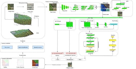
3.1. Overall Workflow

The individual tree segmentation and identification algorithm consist of five parts: data pre-processing, network training, canopy prediction, extraction of contours and centers, as well as accuracy evaluation. As shown in Figure 3, first of all, the UAV images were placed into the dataset by a list of 3D reconstruction, sample tagging and image cutting. The sample and labeled images then were introduced to the mask R-CNN network for training, and at the same time, the corresponding parameters were adjusted to the best condition. Lastly, the optimal model was selected to predict the individual tree crown on the entire aerial orthophoto, extract the contour and center of the tree and calculate the canopy area.

3.2. Mask R-CNN and the Improved Model

3.2.1. Mask R-CNN

Mask R-CNN is a classical instance segmentation model proposed by He [33]. The framework of the network is based on the Faster R-CNN [32] with the addition of a semantic segmentation branch-mask that determines the range of each RoI and achieves the recognition and detection of target contours at the pixel levels. The network’s output is converted from classification--regression to classification--regression--segmentation for the multi-target object detection, recognition and segmentation. The structure of Mask R-CNN includes backbone network layer (Backbone), region proposal network (RPN) layer, RoI align layer (RoIAlign), and bounding box (bbox) as well as classification and masks. As shown in Figure 4, the network’s input is a set of RGB images with 1024 × 1024 pixels, and the feature maps are generated by the feature extraction of ResNet101 [51] and the FPN. The RoI then maps the feature vectors with fixed dimensions in the PRN and RoIAlign layers. Eventually, a segmentation map was obtained on the basis of RoI by utilizing a classifier, a border reviser and a mask generator.

3.2.2. Network Improvements

Because there is a long path between upper and lower features, the location information of lower features may not be well works in multivariate object segmentation, which ultimately reduces the fusion efficiency between upper and lower features [52,53]. Moreover, the loss function of the mask relies only on the region extraction information but ignores the prediction loss of the boundary that yields poor segmentation and recognition results for multiple targets covering each other. Therefore, the following improvements are made to the network:

(a)

Modification of the fusion style

A top-down approach is adopted to fuse the features between the upper and the low levels in the classical Mask R-CNN network. In this way, the single object segmentation needed for classification can be assigned to the FPN network without any loss of features. However, for the large-scale multi-target segmentation, the fusion path between the low-level and the high-level features of the FPN reaches more than 100 levels, for example, the blue dashed line in Figure 5a. This long path can cause underutilization of the features in the low levels [46]. Therefore, a bottom-up approach is applied on features fusion between different levels to shorten the path of features and enhance the utilization of the bottom-level features. As shown in Figure 5b, the bottom-up path is a layer-by-layer iterative process that terminates after reaching the top layer. As a result, the feature fusion path from lower to higher layers can reach between 5 and 10 layers (as shown in the red dashed line), which largely reduces the feature information fusion path between lower and higher layer features. The improved FPN network stores the pinpointed signals and enhances the feature pyramid architecture, thus enabling finer multi-target segmentation.

(b)

Evolution of loss function L_mask

In the loss calculation of Mask R-CNN, each RoI outputs with a corresponding binary mask, and the loss of the mask is a part of the loss in the entire network. To gain the number of categories and the image size, the mask branch encodes an output matrix of size K × m² for each RoI, where K is the number of categories. Combined with the sigmoid function applied to each single pixel, the mask loss is defined as the average binary cross-entropy loss function L_mask. When RoI belongs to the kth category, L_mask only considers the loss caused by the kth mask to it, while the other mask inputs do not contribute to this loss function, decoupling the dependency between category prediction and mask to some extent.

$${\mathrm{L}}_{\mathrm{mask}}=-{\mathsf{\Sigma }}_{\mathrm{k}}\mathrm{k} \log (1- \hat{\mathrm{k}})+(1-\mathrm{k})\log (1- \hat{\mathrm{k}})$$

(1)

However, the cross-entropy loss function ignores the prediction loss of the boundary in the segmentation task, which reduces the accuracy of segmenting the boundary [54]. Since the segmentation task in this study is a densely distributed and irregularly edged individual tree crown, which requires high segmentation accuracy for the boundary, thereby we add the boundary weighted loss (BWL) function to L_mask. During the training process, BWL regularizes the position, shape and continuity of the segmentation using distance loss L_dist to make it closer to the target boundary. The optimized L_mask-bwl is defined as:

$${\mathrm{L}}_{\mathrm{mask}-\mathrm{bwl}}={\mathrm{L}}_{\mathrm{dis}}+{\mathrm{L}}_{\mathrm{mask}}={\mathsf{\alpha }\mathsf{\Sigma }}_{ \hat{\mathrm{y}}\in \mathrm{B}}{ \hat{\mathrm{y}} \mathrm{M}}_{\mathrm{dist}}\left(\mathrm{y}\right)-{\mathsf{\Sigma }}_{ \hat{\mathrm{y}}\in \mathrm{R}}\mathrm{ylog}\left(\hat{\mathrm{y}}\right)+\left(1-\mathrm{y}\right)\log \left(1-\hat{\mathrm{y}}\right)$$

(2)

3.3. Outline and Center Extraction

The simulated canopy for different species is shown in Figure 6a in a way of different color masks. Firstly, the solid closed surfaces are classified and grayed out to different types of images (Figure 6b) by using a color classifier. Next, the grayscale image is scanned using the raster scan method to extract the boundary starting points. Assuming that the input image is F(i, j) = {f_ij}, when a pixel is scanned with grayscale value f_ij ≠ 0, we can check whether it is a starting point on the boundary:

if (fij = 1 & fi,j−1 = 0):

{

(i,j) is the starting point of the outer boundary;

(i2,j2) = (i,j−1);

}

else

{

Continue scanning grating;

}

According to its starting boundary point f_ij, a hollow boundary can be produced by utilizing the boundary tracking algorithm [55], and then restoring its color before graying to yield each solid surface contour as Figure 6c.

In the binarized graph, the zero-order moments M₀₀ and first-order matrices M₁₀, M₀₁ are defined as follows.

$${\mathrm{M}}_{00}={\Sigma }_i{\Sigma }_j\mathrm{F}\left(i,j\right)$$

(3)

$${\mathrm{M}}_{10}={\Sigma }_i{\Sigma }_{j}i · \mathrm{F}\left(i,j\right),{ \mathrm{M}}_{01}={\Sigma }_i{\Sigma }_{j}j · \mathrm{F}\left(i,j\right)$$

(4)

Since F(i,j) is the sum of the grayscale values of all contour pixels, and in the binarized graph, all-white as 1 and all-black as 0, M₀₀ is the sum of the pixel values representing all-white regions. Similarly, the first-order matrix M₁₀ represents the sum of x-coordinates of all-white area pixels, and M₀₁ represents the sum of y-coordinates of all-white areas. Using first-order moments, we can obtain the coordinates of the center of gravity of the graph, which is given as follows:

$${\mathrm{x}}_{\mathrm{c}}=\frac{{\mathrm{M}}_{10}}{{\mathrm{M}}_{00}},{ \mathrm{y}}_{\mathrm{c}}=\frac{{\mathrm{M}}_{01}}{{\mathrm{M}}_{00}}$$

(5)

3.4. Evaluation Index

In this study, four evaluation metrics were used to assess the accuracy of individual tree stand measurement, including Precision, Recall, F1-score and mean average precision (mAP).

$${ \mathrm{P}}_{\mathrm{re}}=\frac{{\mathrm{T}}_{\mathrm{P}}}{{\mathrm{T}}_{\mathrm{P}}+{\mathrm{F}}_{\mathrm{P}}}\times 100\%$$

(6)

$${\mathrm{R}}_{\mathrm{ec}}=\frac{{\mathrm{T}}_{\mathrm{P}}}{{\mathrm{T}}_{\mathrm{P}}+{\mathrm{F}}_{\mathrm{N}}}\times 100\%$$

(7)

$$\mathrm{F}1-\mathrm{score}=\frac{2{\mathrm{P}}_{\mathrm{re}} · {\mathrm{R}}_{\mathrm{ec}}}{2{\mathrm{P}}_{\mathrm{re}}+{\mathrm{R}}_{\mathrm{ec}}}\times 100\%$$

(8)

$$\mathrm{mAP} =\frac{{\Sigma }_1^{\mathrm{m}}{\int }_0^1{\mathrm{P}}_{\mathrm{re}}\left({\mathrm{R}}_{\mathrm{ec}}\right){\mathrm{dR}}_{\mathrm{ec}}}{\mathrm{m}}$$

(9)

Here, T_P is the number of trees correctly identified, F_P is the number of trees incorrectly identified, F_N is the number of trees incorrectly identified as other species, and T_N is the number of trees correctly identified as other species.

Four metrics were used for canopy classification accuracy evaluation, including Kappa coefficient, overall classification accuracy (overall), producer’s accuracy and user’s accuracy [56].

$$\mathrm{Kappa} =\frac{{\mathrm{P}}_0-{ \mathrm{P}}_{\mathrm{e}}}{1-{\mathrm{P}}_{\mathrm{e}}}\times 100\%$$

(10)

$$\mathrm{Overall} =\frac{{\mathrm{T}}_{\mathrm{P}}+{\mathrm{T}}_{\mathrm{N}}}{{\mathrm{T}}_{\mathrm{P}}+{\mathrm{T}}_{\mathrm{N}}+{\mathrm{F}}_{\mathrm{P}}+{\mathrm{F}}_{\mathrm{N}}}\times 100\%$$

(11)

$$\mathrm{Producer}’\mathrm{s} \mathrm{accuracy} =\frac{{\mathrm{x}}_{ii}}{{{\displaystyle \Sigma }}_{j=0}^{\mathrm{n}}{\mathrm{x}}_{ij}}$$

(12)

$$\mathrm{User}’\mathrm{s} \mathrm{accuracy} =\frac{{\mathrm{x}}_{jj}}{{{\displaystyle \Sigma }}_{i=0}^{\mathrm{m}}{\mathrm{x}}_{ij}}$$

(13)

where P₀ is the number of pixels correctly predicted as the number of canopy pixels and divided by the number of total canopy pixels, X_ij is the number of pixels predicted as a certain tree species, P_e is equal to a₁ × b₁ + a₂ × b₂ + … + a_c × b_c/n × n, where ai represents the number of true samples and bi represents the number of samples predicted.

3.5. Network Training and a Comparison with Different Models

The network training parameters have an unparalleled impact on the model training and prediction. In this experiment, when the learning rate was adjusted to 1 × e⁻⁴, the batch size was set to 32, and the epoch was set to 600 times with each epoch of 200 steps, the model accuracy reached the highest level. For the software platform, tensorflow-gpu-1.15 and keras-2.3.1 under Linux system were used as the deep learning framework, and the whole algorithm process was implemented through python. The hardware attributes of the workstation are shown in

Table 4. Workstation hardware attribute.

Hardware	Attribute
CPU	i9-10850
GPU	GTX 2080Ti 11GB
SSD	1T SSD
Memory	64GB

, which is configured with Intel i9-10850 central processing unit (CPU), NVIDIA GTX 2080Ti graphics processor unit (GPU), 1T solid-state drive and 64GB RAM.

In order to verify the accuracy of the improved Mask R-CNN for individual tree extraction, a comparison with other popular image segmentation networks in terms of classification and counting is necessary. U-net and YOLOv3 are also deep learning models based on convolutional neural networks, which can efficiently train self-produced data sets and achieve high accuracy image segmentation models [57,58]. Both approaches have also been repeatedly used for extraction and segmentation in forestry and have achieved high accuracy scores [6,40]. Hence, U-net, YOLOv3 and Mask R-CNN are used in the following for training and prediction of tree crowns to achieve a segmentation performance comparison with the improved Mask R-CNN.

4. Results

4.1. Accuracy Evaluation of Individual Tree Crown Segmentation

In accordance with the results of canopy segmentation and field survey data, various metrics such as precision, recall ratio, F1-score and mAP of each tree species were calculated. Comparing the data in

Table 5. Accuracy evaluation of number prediction in different tree species.

Type	Species	Precision (%)	Recall (%)	F1-Score (%)	Mean Average Precision (%)
Coniferous forest	Pinus armandii	90.28	89.87	90.07	90.39
	Ginkgo biloba	93.21	91.78	92.48	91.23
	Pinus tabulaeformis	92.45	88.71	90.54	90.14
Broadleaf forest	Sophora japonica	80.62	83.42	81.99	80.72
	Salix matsudana	85.44	82.63	84.01	83.68
	Ailanthus altissima	81.97	80.02	80.90	80.06
	Amygdalus davidiana	82.59	80.52	81.54	81.77
	Populus nigra	75.76	77.23	76.98	75.55

, it can be concluded that Pinus armandii, Ginkgo biloba and Pinus tabulaeformis had superior segmentation results, with their precision and recall ratio greater than 88%, and F1-score and mAP higher than 90%. Meanwhile, the precision and recall ratio of Sophora japonica, Salix matsudana, Ailanthus altissima, Amygdalus davidiana ranged between 80.02% and 85.44%, and the F1-score and mAP between 80% and 84%, slightly lower than those of coniferous species. The prediction results of Populus nigra were deficient, with the precision and recall ratio within 77%, and the F1-score and mAP within 75%.

In addition, Figure 7 shows the application of a subset of orthophotos that contains two categories of broad-leaved species (Sophora japonica and Salix matsudana) and one category of coniferous species (Pinus tabulaeformis). The canopy’s bounding box, mask and center of gravity were extracted and shown respectively in Figure 7b–d. The overall results illustrate that the model is superior in identifying coniferous species than broad-leaved species. In particular, the difference between the two maps was about 10%.

4.2. Species Identification and Classification Accuracy Evaluation

The producer’s accuracy and user’s accuracy respectively depict the probability of a true pixel being correctly predicted and the probability of a correct value in the predicted pixels for a particular species. As shown in

Table 6. Comparison of user’s and producer’s accuracy at crown delineation distributed in various tree species ¹.

Prediction Data	Reference Data
	Pinus armandii	Ginkgo biloba	Pinus tabulaeformis	Sophora japonica	Salix matsudana	Ailanthus altissima	Amygdalus davidiana	Populus nigra	Background	User’s accuracy
Pinus armandii	2.599	0.038	0.076	0.022	0	0	0.019	0	0.415	0.82
Ginkgo biloba	0.234	8.971	0.17	0.010	0	0.010	0	0.010	1.270	0.84
Pinus tabulaeformis	0.127	0.102	10.35	0.051	0.038	0.012	0.025	0.012	2.057	0.81
Sophora japonica	0.035	0.023	0.011	8.822	0.023	0.186	0.140	0.233	2.193	0.75
Salix matsudana	0.096	0.032	0	0.064	7.643	0.160	0.245	0.128	2.309	0.71
Ailanthus altissima	0.007	0.037	0.007	0.014	0.185	5.49	0.133	0.185	1.359	0.74
Amygdalus davidiana	0.049	0.037	0.012	0	0.111	0.223	8.949	0.174	2.858	0.72
Populus nigra	0.049	0.033	0.066	0.398	0.082	0.099	0.082	12.60	3.168	0.76
Background	0.015295	0.12236	0.1560	0.03	0.091	0.122	0.214	0.061	29.764	0.97
Producer’s accuracy	0.80	0.9	0.95	0.93	0.93	0.87	0.91	0.93	0.65	-

¹ The measurement unit of prediction and reference data is 9.000 × 10⁶ pixel.

, both producer accuracy and user accuracy of canopy segmentation for each tree species were higher than 0.70 when the field survey data was used for reference. In terms of user accuracy, the distribution range of coniferous canopy was 0.81–0.84 and that of the broadleaf canopy was 0.71–0.76, implying that the image pixels of coniferous species were correctly segmented better than broadleaf species. However, in terms of producer accuracy, the distributions of two species were similar, with the prediction accuracy of coniferous trees ranging from 0.8 to 0.95, and that of broadleaf trees from 0.87 to 0.93. Furthermore, the analysis of the overall accuracy and kappa coefficient in the entire region will be shown later in the discussion section.

4.3. Accuracy Evaluation of Tree Count Detection

To some extent, the accuracy of tree count determines biomass assessment in the whole forest area. The numbers of all tree species measured by field survey and prediction approach are shown in Figure 8, which shows that the average error of coniferous species (3.7%) is smaller than that of broad-leaved species (7.9%). Pinus armandii had the smallest mean error of 2.1%, and Populus nigra had the largest mean error of 9.6%, meanwhile, the total number of trees in the field survey for the whole study area was 52,737 and that of the predicted tree was 50,041, with the overall error (5.11%). This further confirms that our new approach meets the statistical requirement of stand number.

Due to the excessive number of trees across the entire area, fitting the area to all canopies would result in an excessive amount of data and would not be necessary [33]. Therefore, we used a subset of images containing all studied tree species, which includes coniferous trees with 246 and broadleaf trees with 238, to fit the distribution of measured and predicted area values for individual tree canopies (Figure 9). The scatter fit curve for the area of three coniferous species was y = 1.253x − 105.9 and the coefficient R-Square reached 0.9921, which implies that the measured canopy area explained 99.21% of the predicted values. The scatter fit curve for the area of five broadleaf species was y = 0.8919x + 1805, and the R-Square reached 0.9741, indicating that the measured canopy area explained 97.14% of the predicted values.

5. Discussion

5.1. Comparison of the Segmentation and Detection Performance of Different Networks

The kappa coefficient and overall accuracy of crown delineation in different models are illustrated in

Table 7. Comparison of kappa coefficient and overall accuracy of crown delineation in different models.

Network Type	Kappa Coefficient		Overall Accuracy (%)
	Training Set	Test Set	Training Set	Test Set
U-net [57]	0.75	0.70	85.42	81.14
YOLOv3 [58]	0.70	0.62	81.56	78.57
Mask R-CNN [33]	0.79	0.76	90.86	89.72
Improved Mask R-CNN	0.81	0.79	92.71	90.13

. Also, Figure 10 shows the results of crown identification and segmentation using the four different networks in junction land of three species shown in Figure 7a. In the canopy segmentation of coniferous species Pinus tabulaeformis (yellow contour), the segmentation results of the four models were close with a low error rate. U-net’s loss of the entire canopy is obvious in the high canopy density segmentation of coniferous species Sophora japonica (red). There are a lot of internal nested and crossover errors in segmentation of Sophora japonica (red) by YOLOv3 and Mask R-CNN, resulting in a large deviation between the total number and the predicted value. The improved Mask R-CNN achieved the best segmentation results with the least loss compared with other models, without clear conditions of internal nesting. It is attributed to the improved loss function using distance loss L_dist to normalize the position, shape and continuity of the densely distributed canopy for segmentation to improve the accuracy of target boundary segmentation. The above results show that compared with other models, our model not only has significant results in coniferous canopy segmentation, but also still has good results in the dense broadleaf canopy.

To compare the accuracy of the different models for area prediction of individual canopies, we fitted the distribution of measured and predicted area values of individual canopy layers using three other models (U-net, YOLOv3, Mask R-CNN) to the subset of images used in Figure 9. As shown in Figure 11, for broadleaf canopies, the U-net actual area interpretation is the lowest compared to YOLOv3 (R-Square = 0.9615) and Mask R-CNN (R-Square = 0.9712), with the coefficient R-Square of 0.9501 and slope of 1.19. For coniferous canopies, the R-Square of the three models differed less, and the minimum coefficient R-Square was YOLOv3 (0.8269). Compared with Figure 9, it can be seen that the improved Mask R-CNN has accurate prediction ability for both conifer and broadleaf, and the advantage is more obvious for broadleaf area prediction (y = 1.253x − 105.9, R-Square = 0.9921). This is due to the modified bottom-up FPN network that optimizes the signal storage and enhances the pyramid structure for feature extraction so that it improves the accuracy of multi-target segmentation.

5.2. Comparison of Training Time and Loss

The number of model parameters will affect the training time, and the training time will affect the segmentation efficiency. By comparing the data in

Table 8. Model parameters and training time for different models.

Network Type	Model Parameters (million)	Time in Each Epoch (s−1)
U-net	31.05	318
YOLOv3	56.78	489
Mask R-CNN	40.76	372
Improved Mask R-CNN	33.47	327

, we can see that the training parameters (33.47 million) of the improved Mask R-CNN were reduced by 17.88% compared to Mask R-CNN (40.76 million) and the parameters time (327 s) of improved Mask R-CNN reduced by 12.09% compared to Mask R-CNN (372 s), which was attributed to the modification of FPN fusion from up-bottom to bottom-up fusion [45,46]. Although our method is at a disadvantage in training time compared with U-net, it still has an overwhelming advantage over U-net with referring to the segmentation evaluation results in Figure 7.

Figure 12 shows the data loss of the classical Mask R-CNN and the improved model in the training process. As the loss function, L_mask was modified to L_mask-bwl, the improved Mask R-CNN had a more considerable reduction in bbox loss, class loss and mask loss, which, therefore, directly and significantly reduced the overall loss and demonstrated the positive production of L_mask-bwl. At the same time, it enhances the effectiveness of previous studies in loss reduction [39,50].

5.3. The Offset Value in the Center of Gravity and the Bounding Box

Figure 13a,b respectively show the horizontal and vertical offsets (dx, dy) on the center of gravity pixels between ground truth values and the predicted value by the improved Mask R-CNN, which records measurement of pixels in the morphological and structural attributes of the forest canopy [59]. The offset demonstrated a distribution centered at zero with a distribution interval of [−5, 5], which implied that the deviation between predicted value on the center of gravity and the real value was within 20 cm. Figure 13c,d shows the offsets between ground truth and length and width predicted from the bounding box of individual trees (d(log(w)), d(log(h)). It can see from the figures that the offsets of the bounding box showed a distribution centered at 4, with the main distribution interval of [0, 10], indicating that the deviation between the predicted values and the ground truth was within 40 cm on the canopy boundary. Combined with previous studies [1,60], the stability in the above deviations satisfied the basic requirements of size measurement in forestry individual tree crown.

5.4. Segmentation Results at Different Brightness Levels

To verify the suitability of the algorithm for extracting individual trees under different conditions, different light intensity environments are simulated by varying the brightness of the images. Assuming that the original image has a light intensity of 1, the images in the brightness interval range [0.5, 1.5] are predicted and segmented, where the step value of the brightness variation is 0.1. The results show that the accuracy of individual tree prediction is higher than 90% when the brightness varies over the range of [0.6, 1.25]. The segmentation results for brightness of 0.5, 0.8, 1, 1.2, 1.4 are shown in Figure 14, which demonstrates that the improved Mask R-CNN model has an excellent environmental utility.

5.5. False Segmentation

The proposed method also has certain inherited drawbacks in individual tree segmentation, and the misspecification of broad-leaved species is higher than that of coniferous, mainly because of the following reasons: (1) As shown in Figure 15b, the whole aerial image dataset is affected by the weather such as light intensity and wind speed on the day of shooting, and there are phenomena such as feature point mismatch and surface texture generation confusion in the process of 3D reconstruction and orthophoto synthesis, which makes the canopy prediction and segmentation with random errors. This phenomenon is also consistent with the findings from Freudenberg et al. [40]. (2) The canopy width was obscured or overlapped between single trees, resulting in some canopy widths not being displayed in the aerial images, such as the false A and B encircled by the black box in Figure 15d. (3) Coniferous tree canopies are simple in shape and consistent in size, and feature points are easy to search, while broad-leaved tree canopies are complex in shape and size, with fewer similar structures, making feature matching more difficult, for example, false C exists in Figure 15d. (4) The distribution of the background data in Table 6 indicates that the loss and misjudgment in tree species canopy are mainly related to the presence of background and False segmentation, and it also can be directly observed in Figure 15b,d.

6. Conclusions

Multi-species individual tree segmentation algorithm based on UAV images can accurately detect and extract the contour, center of gravity, canopy area, and the number of each species by utilizing the improved Mask R-CNN. In the modification of the model, the optimized FPN network stores the accurate signal and shortens the training time by enhancing the feature pyramid structure for a more efficient multi-target segmentation. Additionally, the modified Lmask-bwl regularizes the position, shape, and continuity of the segmentation using the distance loss L_dist to make it closer to the target boundary. Based on the test results, the individual tree segmentation and identification accuracy of the three coniferous and five broadleaf species satisfied the requirements in forestry engineering measurement. Meanwhile, in comparison with other image segmentation networks (U-net, YOLOv3, and Mask R-CNN), the improved Mask R-CNN in multi-species tree classification has the highest overall accuracy (90.13%) and kappa coefficient (0.79). The proposed method has more advantages over the other three networks for canopy segmentation and counting of broad-leaved tree species. Nevertheless, the algorithm in this study is still affected by the environment and the complexity of the canopy, and there are subtle segmentation errors in the individual tree segmentation. The currently constructed model only focused on canopy segmentation and statistics under planar images but was not explored in the DSM model. Future studies will be focused on studying the DSM model using a 3D-Mask-R-CNN network for extracting and measuring tree height.

References

1. Wagner, F.H.; Ferreira, M.P.; Sanchez, A.; Hirye, M.C.M.; Zortea, M.; Gloor, E.; Phillips, O.L.; Filho, C.R.d.S.; Shimabukuro, Y.E.; Aragão, L.E.O.C. Individual Tree Crown Delineation in a Highly Diverse Tropical Forest Using Very High Resolution Satellite Images. ISPRS J. Photogramm. Remote Sens. 2018, 145, 362–377. [Google Scholar] [CrossRef]
2. Lindquist, E.J.; D’Annunzio, R.; Gerrand, A.; MacDicken, K.; Achard, F.; Beuchle, R.; Brink, A.; Eva, H.D.; Mayaux, P.; San-Miguel-Ayanz, J.; et al. Global Forest Land-Use Change 1990–2005; FAO Forestry Paper: Rome, Italy, 2012. [Google Scholar]
3. Crowther, T.W.; Glick, H.B.; Covey, K.R.; Bettigole, C.; Maynard, D.S.; Thomas, S.M.; Smith, J.R.; Hintler, G.; Duguid, M.C.; Amatulli, G.; et al. Mapping Tree Density at a Global Scale. Nature 2015, 525, 201–205. [Google Scholar] [CrossRef] [PubMed]
4. Diez, Y.; Kentsch, S.; Fukuda, M.; Caceres, M.L.L.; Moritake, K. Deep Learning in Forestry Using UAV-Acquired RGB Data: A Practical Review. Remote Sens. 2021, 13, 2837. [Google Scholar] [CrossRef]
5. Wang, L.; Gong, P.; Biging, G.S. Individual Tree-Crown Delineation and Treetop Detection in High-Spatial-Resolution Aerial Imagery. Photogramm. Eng. Remote Sens. 2004, 70, 351–358. [Google Scholar] [CrossRef] [Green Version]
6. Santos, A.A.d.; Marcato, J., Jr.; Araújo, M.S.; Di Martini, D.R.; Tetila, E.C.; Siqueira, H.L.; Aoki, C.; Eltner, A.; Matsubara, E.T.; Pistori, H.; et al. Assessment of CNN-Based Methods for Individual Tree Detection on Images Captured by RGB Cameras Attached to UAVs. Sensors 2019, 19, 3595. [Google Scholar] [CrossRef] [PubMed] [Green Version]
7. Miraki, M.; Sohrabi, H.; Fatehi, P.; Kneubuehler, M. Individual Tree Crown Delineation from High-Resolution UAV Images in Broadleaf Forest. Ecol. Inform. 2021, 61, 101207. [Google Scholar] [CrossRef]
8. Dainelli, R.; Toscano, P.; Gennaro, S.F.D.; Matese, A. Recent Advances in Unmanned Aerial Vehicle Forest Remote Sensing—A Systematic Review. Part I: A General Framework. Forests 2021, 12, 327. [Google Scholar] [CrossRef]
9. Harikumar, A.; Bovolo, F.; Bruzzone, L. A Local Projection-Based Approach to Individual Tree Detection and 3-D Crown Delineation in Multistoried Coniferous Forests Using High-Density Airborne LiDAR Data. IEEE Trans. Geosci. Remote Sens. 2019, 57, 1168–1182. [Google Scholar] [CrossRef]
10. Zhang, B.; Zhao, L.; Zhang, X. Three-Dimensional Convolutional Neural Network Model for Tree Species Classification Using Airborne Hyperspectral Images. Remote Sens. Environ. 2020, 247, 111938. [Google Scholar] [CrossRef]
11. Modzelewska, A.; Kamińska, A.; Fassnacht, F.E.; Stereńczak, K. Multitemporal Hyperspectral Tree Species Classification in the Biaowiea Forest World Heritage Site. Forestry 2021, 94, 464–476. [Google Scholar] [CrossRef]
12. Liu, K.; Wang, A.; Zhang, S.; Zhu, Z.; Bi, Y.; Wang, Y.; Du, X. Tree Species Diversity Mapping Using UAS-Based Digital Aerial Photogrammetry Point Clouds and Multispectral Imageries in a Subtropical Forest Invaded by Moso Bamboo (Phyllostachys Edulis). Int. J. Appl. Earth Obs. Geoinform. 2021, 104, 102587. [Google Scholar] [CrossRef]
13. Tochon, G.; Féret, J.B.; Valero, S.; Martin, R.E.; Knapp, D.E.; Salembier, P.; Chanussot, J.; Asner, G.P. On the Use of Binary Partition Trees for the Tree Crown Segmentation of Tropical Rainforest Hyperspectral Images. Remote Sens. Env. 2015, 159, 318–331. [Google Scholar] [CrossRef] [Green Version]
14. Lee, J.; Cai, X.; Lellmann, J.; Dalponte, M.; Malhi, Y.; Butt, N.; Morecroft, M.; Schönlieb, C.-B.; Coomes, D.A. Individual Tree Species Classification from Airborne Multisensor Imagery Using Robust PCA. IEEE J. Sel. Top. Appl. Earth Obser. Remote Sens. 2016, 9, 2554–2567. [Google Scholar] [CrossRef] [Green Version]
15. Jing, L.; Hu, B.; Noland, T.; Li, J. An Individual Tree Crown Delineation Method Based on Multi-Scale Segmentation of Imagery. ISPRS J. Photogramm. Remote Sens. 2012, 70, 88–98. [Google Scholar] [CrossRef]
16. Zhang, J.; Sohn, G.; Bredif, M. A Hybrid Framework for Single Tree Detection from Airborne Laser Scanning Data: A Case Study in Temperate Mature Coniferous Forests in Ontario, Canada. J. Photogramm. Remote Sens. 2014, 98, 44–57. [Google Scholar] [CrossRef] [Green Version]
17. Liu, T.; Im, J.; Lindi, J.Q. A Novel Transferable Individual Tree Crown Delineation Model Based on Fishing Net Dragging and Boundary Classification. ISPRS J. Photogramm. Remote Sens. 2015, 110, 34–47. [Google Scholar] [CrossRef]
18. Cho, M.A.; Malahlela, O.; Ramoelo, A. Assessing the Utility Worldview-2 Imagery for Tree Species Mapping in South African Subtropical Humid Forest and the Conservation Implications: Dukuduku Forest Patch as Case Study. Int. J. Appl. Earth Obser. Geoinform. 2015, 38, 349–357. [Google Scholar] [CrossRef]
19. Mutanga, O.; Adam, E.; Cho, M.A. High Density Biomass Estimation for Wetland Vegetation Using Worldview-2 Imagery and Random Forest Regression Algorithm. Int. J. Appl. Earth Obser. Geoinform. 2012, 18, 399–406. [Google Scholar] [CrossRef]
20. Schiefer, F.; Kattenborn, T.; Frick, A.; Frey, J.; Schall, P.; Koch, B.; Schmidtlein, S. Mapping Forest Tree Species in High Resolution UAV-Based RGB-Imagery by Means of Convolutional Neural Networks. ISPRS J. Photogramm. Remote Sens. 2020, 170, 205–215. [Google Scholar] [CrossRef]
21. Asner, G.P.; Martin, R.E.; Knapp, D.E.; Tupayachi, R.; Anderson, C.B.; Sinca, F.; Vaughn, N.R.; Llactayo, W. Airborne Laser-Guided Imaging Spectroscopy to Mapforest Trait Diversity and Guide Conservation. Science 2017, 355, 385–389. [Google Scholar] [CrossRef]
22. Su, A.; Qi, J.; Huang, H. Indirect Measurement of Forest Canopy Temperature by Handheld Thermal Infrared Imager through Upward Observation. Remote Sens. 2020, 12, 3559. [Google Scholar] [CrossRef]
23. Brandt, M.; Tucker, C.J.; Kariryaa, A.; Ransmussen, K.; Abel, C.; Small, J.; Chave, J.; Rasmussen, L.V.; Hiernaux, P.; Diouf, A.A.; et al. An Unexpectedly Large Count of Trees in the West African Sahara and Sahel. Nature 2020, 587, 78–82. [Google Scholar] [CrossRef] [PubMed]
24. Chadwick, A.J.; Goodbody, T.R.H.; Coops, N.C.; Hervieux, A.; Bater, C.W.; Martens, L.A.; White, B.; Röeser, D. Automatic Delineation and Height Measurement of Regenerating Conifer Crowns under Leaf-Off Conditions Using UAV Imagery. Remote Sens. 2020, 12, 4104. [Google Scholar] [CrossRef]
25. Fujimoto, A.; Haga, C.; Matsui, T.; Machimura, T.; Hayashi, K.; Sugita, S.; Takagi, H. An End to End Process Development for UAV-SfM Based Forest Monitoring: Individual Tree Detection, Species Classification and Carbon Dynamics Simulation. Forests 2019, 10, 680. [Google Scholar] [CrossRef] [Green Version]
26. Egli, S.; Höpke, M. CNN-Based Tree Species Classification Using High Resolution RGB Image Data from Automated UAV Observations. Remote Sens. 2020, 12, 3892. [Google Scholar] [CrossRef]
27. Tran, D.Q.; Park, M.; Jung, D.; Park, S. Damage-Map Estimation Using UAV Images and Deep Learning Algorithms for Disaster Management System. Remote Sens. 2020, 12, 4169. [Google Scholar] [CrossRef]
28. Safonova, A.; Tabik, S.; Alcaraz-Segura, D.; Rubtsov, A.; Maglinets, Y.; Herrera, F. Detection of Fir Trees (Abies Sibirica) Damaged by the Bark Beetle in Unmanned Aerial Vehicle Images with Deep Learning. Remote Sens. 2019, 11, 643. [Google Scholar] [CrossRef] [Green Version]
29. Cao, K.; Zhang, X. An Improved Res-UNet Model for Tree Species Classification Using Airborne High-Resolution Images. Remote Sens. 2020, 12, 1128. [Google Scholar] [CrossRef] [Green Version]
30. Szegedy, C.; Liu, W.; Jia, Y.; Sermanet, P.; Reed, S.; Anguelov, D.; Erhan, D.; Vanhoucke, V.; Rabinovich, A. Going Deeper with Convolutions. In Proceedings of the IEEE Conference on Computer Vision and Pattern Recognition (CVPR), Boston, MA, USA, 7–12 June 2015. [Google Scholar] [CrossRef] [Green Version]
31. Osco, L.P.; Arruda, M.S.; Gonçalves, D.N.; Dias, A.; Batistoti, J.; Souza, M.; Gomes, F.D.G.; Ramos, A.P.M.; Jorge, L.A.C.; Liesenberg, V.; et al. A CNN Approach to Simultaneously Count Plants and Detect Plantation-Rows from UAV Imagery. ISPRS J. Photogramm. Remote Sens. 2021, 174, 1–17. [Google Scholar] [CrossRef]
32. Ren, S.; He, K.; Girshick, R.; Sun, J. Faster R-CNN: Towards Real-Time Object Detection with Region Proposal Networks. IEEE Trans. Pattern Anal. Mach. Intell. 2017, 39, 1137–1149. [Google Scholar] [CrossRef] [Green Version]
33. He, K.; Gkioxari, G.; Dollár, P.; Girshick, R. Mask R-CNN. IEEE Trans. Pattern Anal. Mach. Intell. 2017, 42, 386–397. [Google Scholar] [CrossRef] [PubMed]
34. Han, Q.; Yin, Q.; Zheng, X.; Chen, Z. Remote Sensing Image Building Detection Method Based on Mask R-CNN. Complex Intell. Syst. 2021, 1–9. [Google Scholar] [CrossRef]
35. Zheng, J.; Fu, H.; Li, W.; Wu, W.; Yu, L.; Yuan, S.; Yuk, W.; William, T.; Pang, T.K.; Kanniah, K.D.; et al. Growing Status Observation for Oil Palm Trees Using Unmanned Aerial Vehicle (UAV) Images. J. Photogramm. Remote Sens. 2021, 173, 95–121. [Google Scholar] [CrossRef]
36. Braga, J.R.G.; Peripato, V.; Dalagnol, R.; Ferreira, M.P.; Tarabalka, Y.; Aragão, L.E.O.C.; Velho, H.F.C.; Shiguemori, E.H.; Wagner, F.H. Tree Crown Delineation Algorithm Based on a Convolutional Neural Network. Remote Sens. 2020, 12, 1288. [Google Scholar] [CrossRef] [Green Version]
37. Yang, D.; Wang, X.; Zhang, H.; Yin, Z.; Su, D.; Xu, J. A Mask R-CNN Based Particle Identification for Quantitative Shape Evaluation of Granular Materials. Powder Technol. 2021, 392, 296–305. [Google Scholar] [CrossRef]
38. Safonova, A.; Guirado, E.; Maglinets, Y.; Domingo, A.-S.; Tabik, S. Olive Tree Biovolume from UAV Multi-Resolution Image Segmentation with Mask R-CNN. Sensors 2021, 21, 1617. [Google Scholar] [CrossRef]
39. Cao, X.; Pan, J.S.; Wang, Z.; Sun, Z.; Haq, A.; Deng, W.; Yang, S. Application of Generated Mask Method Based on Mask R-CNN in Classification and Detection of Melanoma. Comput. Methods Programs Biomed. 2021, 207, 106174. [Google Scholar] [CrossRef]
40. Freudenberg, M.; Nölke, N.; Agostini, A.; Urban, K.; Wörgötter, F.; Kleinn, C. Large Scale Palm Tree Detection in High Resolution Satellite Images Using U-Net. Remote Sens. 2019, 11, 312. [Google Scholar] [CrossRef] [Green Version]
41. Chu, P.; Li, Z.; Lammers, K.; Lu, R.; Liu, X. Deep learning-based apple detection using a suppression mask R-CNN. Pattern Recognit. Lett. 2021, 147, 206–211. [Google Scholar] [CrossRef]
42. Loh, D.R.; Wen, X.Y.; Yapeter, J.; Subburaj, K.; Chandramohanadas, R. A Deep Learning Approach to the Screening of Malaria Infection: Automated and Rapid Cell Counting, Object Detection and Instance Segmentation Using Mask R-CNN. Comput. Med. Imaging Graph. 2021, 88, 10185. [Google Scholar] [CrossRef]
43. Huang, G.; Liu, Z.; Van Der Maaten, L.; Weinberger, K.Q. Densely connected convolutional networks. In Proceedings of the 2017 IEEE Conference on Computer Vision and Pattern Recognition, Honolulu, HI, USA, 21–26 July 2017. [Google Scholar] [CrossRef] [Green Version]
44. Chen, J.; Yuan, Z.; Peng, J.; Chen, L.; Huang, H.; Zhu, J.; Liu, Y.; Li, H. DASNet: Dual Attentive Fully Convolutional Siamese Networks for Change Detection in High-Resolution Satellite Images. IEEE J. Sel. Top. Appl. Earth Obs. Remote Sens. 2021, 14, 1194–1206. [Google Scholar] [CrossRef]
45. Zimmermann, R.S.; Siems, J.N. Faster Training of Mask R-CNN by Focusing on Instance Boundaries. Comput. Vis. Image Underst. 2019, 188, 102795. [Google Scholar] [CrossRef] [Green Version]
46. Liu, S.; Qi, L.; Qin, H.; Shi, J.; Jia, J. Path Aggregation Network for Instance Segmentation. In Proceedings of the 2018, IEEE/CVF Conference on Computer Vision and Pattern Recognition (CVPR), Salt Lake City, UT, USA, 18–23 June 2018; Institute of Electrical and Electronics Engineers (IEEE): New York, NY, USA, 2018; pp. 8759–8768. [Google Scholar] [CrossRef] [Green Version]
47. ContextCapture Software, v4.4.11; Bentley: Exton, PA, USA. Available online: https://www.bentley.com/zh/products/brands/contextcapture(accessed on 1 December 2018).
48. ArcGIS Desktop Software, v10.4; ESRI: Redlands, CA, USA. Available online: https://www.esri.com/(accessed on 12 June 2021).
49. VGG Image Annotator Software, v1.0; VGG: Oxford, UK. Available online: https://www.robots.ox.ac.uk/~vgg/software/via/via.html(accessed on 22 July 2017).
50. Photoshop Software, Berkeley, CA, USA, v2019. Adobe. Available online: https://www.adobe.com/products/photoshop.html(accessed on 16 October 2018).
51. He, K.; Zhang, X.; Ren, S.; Sun, J. Deep Residual Learning for Image Recognition. In Proceedings of the 2016 IEEE Conference on Computer Vision and Pattern Recognition (CVPR), Las Vegas, NV, USA, 27–30 June 2016. [Google Scholar]
52. Luc, P.; Couprie, C.; Lecun, Y.; Verbeek, J. Predicting Future Instance Segmentation by Forecasting Convolutional Features. In Proceedings of the European Conference on Computer Vision, Munich, Germany, 8–14 September 2018. [Google Scholar] [CrossRef] [Green Version]
53. Zhang, Z.; Zhang, X.; Peng, C.; Cheng, D.; Sun, J. ExFuse: Enhancing Feature Fusion for Semantic Segmentation. In Proceedings of the European Conference on Computer Vision, Munich, Germany, 8–14 September 2018. [Google Scholar]
54. Zhu, Q.; Du, B.; Yan, P. Boundary-Weighted Domain Adaptive Neural Network for Prostate MR Image Segmentation. IEEE Trans. Med. Imaging 2019, 99, 1. [Google Scholar] [CrossRef] [PubMed]
55. Suzuki, S.; Be, K. Topological Structural Analysis of Digitized Binary Images by Border Following. Comput. Vis. Graph. Image Process. 1985, 30, 32–46. [Google Scholar] [CrossRef]
56. Shao, G.; Tang, L.; Liao, J. Overselling Overall Map Accuracy Misinforms about Research Reliability. Landsc. Ecol. 2019, 34, 2487–2492. [Google Scholar] [CrossRef] [Green Version]
57. Ronneberger, O.; Fischer, P.; Brox, T. U-Net: Convolutional Networks for Biomedical Image Segmentation. In Proceedings of the International Conference on Medical Image Computing and Computer-Assisted Intervention, Munich, Germany, 5–9 October 2015. [Google Scholar] [CrossRef] [Green Version]
58. Redmon, J.; Farhadi, A. YOLOv3: An Incremental Improvement. arXiv 2018, arXiv:1804.02767. [Google Scholar]
59. Ferreira, M.P.; Zortea, M.; Zanotta, D.C.; Shimabukuro, Y.E.; de Souza Filho, C.R. Mapping Tree Species in Tropical Seasonal Semi-Deciduous Forests with Hyperspectral and Multispectral Data. Remote Sens. Environ. 2016, 179, 66–78. [Google Scholar] [CrossRef]
60. Ferreira, M.P.; Wagner, F.H.; Aragão, L.; Shimabukuro, Y.E.; Filho, C.R.S. Tree Species Classification in Tropical Forests Using Visible to Shortwave Infrared WorldView-3 Images and Texture Analysis. ISPRS J. Photogramm. Remote Sens. 2019, 149, 119–131. [Google Scholar] [CrossRef]
Figure 1. (a) Location of the study area in China; (b) Changping District of Beijing with plains and hills as the main landform; (c) satellite map site near the study area; (d) Digital surface model (DSM) of the study area; (e) Digital orthophoto map (DOM) synthesized from drone images.
Remotesensing 14 00874 g001
Figure 2. (a) GPS points from field sampling; (b) Sample images and ground truth. The orange, green and blue borders in (b) are the ground truth, respectively, and the numbers on the bounding boxes are the category labels; (c) Sampling area selected from the study area; (d) Various tree species of study area.
Remotesensing 14 00874 g002
Figure 3. Algorithm flow in segmentation and identification for individual tree.
Remotesensing 14 00874 g003
Figure 4. The structure workflow in Mask R-CNN network.
Remotesensing 14 00874 g004
Figure 5. Feature fusion path of the improved FPN. (a) top-down (b) bottom-up.
Remotesensing 14 00874 g005
Figure 6. (a) Simulation of canopy of different tree species. (b) Canopy classification of different tree species. (c) Contour extraction of individual canopy. (d) Contour and center extraction of individual canopy.
Remotesensing 14 00874 g006
Figure 7. (a) Input image; (b) Bbox prediction; (c) Mask prediction; (d) Center of gravity prediction.
Remotesensing 14 00874 g007
Figure 8. Comparison of field survey data and predicted data for the number of eight species.
Remotesensing 14 00874 g008
Figure 9. Fitting curves of predicted and real values of canopy area. (a) Conifer the improved Mask R-CNN. (b) Broadleaf the improved Mask R-CNN.
Remotesensing 14 00874 g009
Figure 10. Tree crown identification and segmentation results by using 4 different networks. (a) U-net, (b) YOLOv3, (c) Mask R-CNN, (d) The improved Mask R-CNN.
Remotesensing 14 00874 g010
Figure 11. Fitting curves of predicted and real values of canopy area by using other networks. (a) Conifer curve fitted by U-net, (b) Broadleaf curve fitted by U-net, (c) Conifer curve fitted by YOLOv3, (d) Broadleaf curve fitted by YOLOv3, (e) Conifer Mask R-CNN, (f) Broadleaf Mask R-CNN.
Remotesensing 14 00874 g011aRemotesensing 14 00874 g011b
Figure 12. (a) The full loss in Mask R-CNN and Improved Mask R-CNN. (b) The bbox loss in Mask R-CNN and Improved Mask R-CNN. (c) The class loss in Mask R-CNN and Improved Mask R-CNN. (d) The mask loss in Mask R-CNN and Improved Mask R-CNN.
Remotesensing 14 00874 g012
Figure 13. (a) The horizontal offset on the center of gravity pixels between ground truth values and the predicted value. (b) The vertical offset on the center of gravity pixels between ground truth values and the predicted value. (c) The offset between ground truth and length predicted from the bounding box of individual trees. (d) The offset between ground truth and width predicted from the bounding box of individual trees.
Remotesensing 14 00874 g013
Figure 14. (a) Original image. (b) Predicted results at a brightness of 0.5. (c) Predicted results at a brightness of 0.8. (d) Predicted results at a brightness of 1. (e) Predicted results at a brightness of 1.2. (f) Predicted results at a brightness of 1.4.
Remotesensing 14 00874 g014
Figure 15. (a,c) Orthographic images. (b,d) Canopy segmentation result and wrong cases.
Remotesensing 14 00874 g015aRemotesensing 14 00874 g015b