Mismatching Removal for Feature-Point Matching Based on Triangular Topology Probability Sampling Consensus

Abstract

Feature-point matching between two images is a fundamental process in remote-sensing applications, such as image registration. However, mismatching is inevitable, and it needs to be removed. It is difficult for existing methods to remove a high ratio of mismatches. To address this issue, a robust method, called triangular topology probability sampling consensus (TSAC), is proposed, which combines the topology network and resampling methods. The proposed method constructs the triangular topology of the feature points of two images, quantifies the mismatching probability for each point pair, and then weights the probability into the random process of RANSAC by calculating the optimal homography matrix between the two images so that the mismatches can be detected and removed. Compared with the state-of-the-art methods, TSAC has superior performances in accuracy and robustness.

1. Introduction

Feature-point matching is an important component of image processing, and it is widely used in remote sensing, including in target recognition, image registration, object tracking, pose estimation, etc. With the applications of image feature-point matching becoming more diverse, its accuracy and robustness are of vital importance.

Therefore, there have been many types of research conducted on the optimization of feature-point matching recently. Generally, this kind of research can be divided into feature extraction and feature-point matching. As for feature extraction, traditionally, many kinds of feature descriptors have been proposed, such as SIFT (scale-invariant feature transform) [1], BRIEF (binary robust independent elementary features) [2], etc. There are also many improved feature points, such as CSIFT [3], SURF [4], and some others that are based on deep neural networks, such as LIFT (learned invariant feature transform) [5], SuperPoint [6], etc., which improve the accuracy and precision to some degree. Feature-point matching calculates the similarities between the feature points in different images and matches them. Many of the feature points are similar in some applications, so mismatches that have a great influence on the accuracy for following the progress, such as image registration or pose estimation, do occur.

Generally, the method of feature extraction is fixed in a certain application after being selected at the start. On the other hand, no matter what feature-point extraction method is employed, there still exists a high ratio of mismatches in some situations. Therefore, the detection and removal of mismatching is an important task for precise and robust feature-point matching.

As for the removal of mismatching, a variety of studies have been carried out. The most famous method is RANSAC (random sample consensus) [7], proposed by Fischler in 1981. Subsequently, many new methods based on RANSAC have been proposed from different perspectives. Generally, these methods for mismatching removal improve the efficiency and accuracy of feature-point matching and perform well in applications with low ratios of mismatching. Nevertheless, there remain difficulties in the applications with high ratios of mismatching. The detailed related works will be introduced in the following sections.

Here, we briefly review the methods for the removal of mismatching, which can be divided into three categories, according to different principles: regression-based, resampling-based, and geometry-based.

1.1. Regression-Based Mismatching Removal

The methods based on regression assume that all correct matching conforms to a specific function model, and they calculate the parameters of the model by regression using each feature-point pair, and finally, they judge each matching, whether it is mismatched or not, by calculating the error in the function model.

The popular method based on regression uses the least squares method, which minimizes the sum of the square errors to find an optimal parameter of the model so that as many matches as possible can satisfy it. Then, it calculates the error of the putative matches in this model, and finally, it makes judgments according to this error.

The process of this method is relatively simple, and the speed of regression is also fast. However, some mismatches with large errors will have an impact on the accuracies of the regression model parameters, which seriously affects the result of the mismatching removal. Moreover, the method needs to provide the regression model manually, and the regression model will affect the accuracy of the mismatching detection.

There are also some optimized methods that have been proposed in recent decades. Li et al. propose subregion least squares iterative fitting [8], which regresses the model and removes the mismatches continuously until the errors of all the matching points meet the threshold. This method improves the matching accuracy. As for regression models, there are also some methods that have been developed, such as polynomial regression, proposed by Niu et al., which performs well in color image mismatching removal [9].

Even though these methods improve the efficiency, the regression-based methods are easily affected by the mismatches with large errors, which makes it difficult to detect mismatches. Therefore, the methods based on regression are not so widely used.

1.2. Geometry-Based Mismatching Removal

In recent years, many studies have focused on combining feature-point matching with the geometries of the feature points to construct the geometric or topological relationships between the feature points to remove mismatching.

GTM (graph transformation matching) [10], proposed by Aguilar et al., is the typical method based on geometry, which constructs the KNN undirected graph on the basis of feature points to remove the mismatches. In our previous work [11], a robust method was proposed, which is based on comparing the triangular topologies of the feature points. Zhu et al. put forward the method, based on the similar structure constraints of the feature points [12]. Luo et al. analyze the relationship of the Euclidean distance between the feature points and then corrects the mismatch on the basis of the angular cosine [13]. Zhao et al. removed the mismatches according to the constraint that the matching distances tend to be consistent [14].

The methods based on geometry constraints or topology can detect mismatches efficiently, and they also have high accuracy, while being not easily affected by mismatches, theoretically. Therefore, these methods have been used on many occasions.

1.3. Resampling-Based Mismatching Removal

The method based on resampling finds the model that makes the maximum number of matches meet the error threshold. In the area of mismatching removal, the most popular method is using RANSAC to calculate the basic matrix, or the homography matrix [15,16], and estimating the optimal matrix of the two images; the outliers of the matrix model are considered the mismatches. However, on account of the uncertain iteration number of RANSAC, the efficiency will be reduced when there are a large number of mismatches. Therefore, more and more methods to improve RANSAC are being proposed, which include the optimization of the sampling, the optimization of the loss function, and the optimization of the model estimation.

The optimization of sampling, such as PROSAC (progressive sampling consensus), first obtains the probability of each piece of data being an inlier, and then preferentially extracts the data with high probabilities in the random process [17]. GroupSAC first groups all the matches, and the group with more matching points is preferred for the sampling [18]. The optimization of the loss function, such as MLESAC (maximum likelihood SAC), proposes a new loss function instead of the function of RANSAC, and enhances the accuracy of the calculation [19]. The optimization of the model estimation, such as R-RANSAC and SPRT-RANSAC, will first judge whether it is the correct model, and will continue to sample and iterate if is not [20,21].

Recently, more improved methods based on resampling have been put forward. USAC (universal RANSAC) is a new universal framework for RANSAC [22]. DL-RANSAC (descendant likelihood RANSAC) introduces descending likelihood to reduce the randomness so that it converges faster than the conventional RANSAC [23]. GMS-RANSAC (grid-based motion RANSAC) divides the initial point sets and removes mismatching for image registration [24]. PCA-SIFT uses PCA to obtain new feature descriptors, sorts them according to the KNN algorithm, and then uses the RANSAC to remove the mismatching [25]. SESAC (sequential evaluation on sample consensus), which performs better than PROSAC, sorts the matches on the basis of the similarities of the corresponding features, and then selects the samples sequentially and obtains the model by the least squares method. [26]. Gao et al. improve the RANSAC by taking prevalidation and resampling during iterations, which accelerates the efficiency [27].

Compared with the method based on regression, the mismatches with large errors have little influence on RANSAC or the other resampling methods. That is, a mismatch with a large error will affect the results calculated by the regression-based method a lot, while influencing the results obtained by the resampling-based method a little, because not all points are required to conform to the model in the resampling-based method. Moreover, at the same time, the method is also adapted to the dataset containing many mismatches. Therefore, the method based on resampling is the most widely used at present.

In conclusion, geometry-based methods and resampling-based methods, and especially the latter one, generally have good results and perform well in the case of a nonhigh ratio of mismatching.

However, in many complex applications, which contain a high ratio of mismatching, the existing methods still cannot work well. The more mismatches that exist, the harder it is to calculate the correct model. Specifically, RANSAC calculates the model by randomly selecting a set of matches and validating it; the correct model can be obtained only when an entirely proper set of matches is selected. When the ratio of mismatches is too high, it is difficult for RANSAC to select the correct point sets randomly.

As for remote-sensing images, they are generally images of the ground landscape taken by satellites at certain altitudes. Usually, the landscape, especially the urban landscape, has a high similarity and repeatability, which results in a lot of mismatches in remote-sensing images.

In this paper, we propose a robust method for mismatching removal, namely, triangular topology probability sampling consensus (TSAC), which adapts to a high mismatching ratio. The contributions of our work can be summarized as follows:

• We propose a mismatching-probability-calculating method based on feature-point triangular topology. The method constructs a topological network of the feature points on the image and then calculates the mismatching probability;
• We propose a new sampling method—probability sampling consensus—which weights the probability calculated above to the random process of the RANSAC so that the mismatches can be detected and removed.

The remainder of this paper is organized as follows: Section 2 describes the related works; Section 3 presents the proposed TSAC method in detail; Section 4 presents the results and an analysis of the experiments; and finally, we draw conclusions in Section 5.

2. Materials and Methods

2.1. Motivation and Main Idea

Here, we analyze the disadvantages of the geometry-based and resampling-based methods. Geometry-based methods have high accuracy for judging whether a pair of matching points correctly correspond or not. Even so, there remain many errors when directly selecting mismatches via the geometry-based method. As for resampling-based methods, they sample four pairs of matching points to calculate the homography matrix and verify it. These methods make full use of the affine invariance that two photos of the same area taken from different poses conform to an affine transformation, which can be concluded as a homography matrix; therefore, they obtain better results. However, when there are too many mismatches, selecting a set of four correct pairs of matching points by a random process is difficult. Therefore, our main idea is to analyze the geometric topologies of feature points to calculate the mismatching probability of a point pair, rather than directly determining whether it is a mismatch. Then, instead of selecting matching points with equal probabilities indiscriminately, we import the mismatching probabilities to the random process of RANSAC, which should improve the success rate.

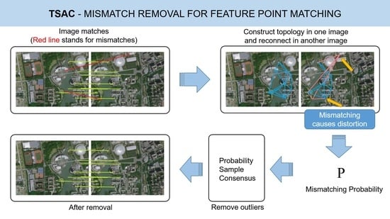
As is shown in Figure 1, the proposed TSAC method includes two stages: first, the construction of a topological network, and then the calculation of the mismatching probability for each point pair, according to the network. There are several types of topological networks, and the triangular topology was chosen in the proposed method. In our previous work [11], it was first used for image mismatching removal. However, we used it to remove mismatches directly in [11], where it is hard to achieve high accuracy in the case of a high mismatching ratio, so we added lots of criteria to find the mismatching, such as the topological constraint and the length constraint, which makes the process of judgment very complex. In this paper, instead of making a direct judgment as to whether a match is incorrect, we calculate the mismatching probability, which does not decrease the mismatches. Therefore, here, we simplify them into a single and simple condition that the mismatching points will lead to the distortion of the topological network, which means that the lines of the network will cross. This is much simpler and more efficient.

Then, we import the probability to the random process of RANSAC. The matches with low mismatching possibilities will have a higher probability of being selected in each random process; thus, we can select the matching points and calculate the correct homography matrix more efficiently so as to remove the mismatching. Although some of the existing methods, e.g., PROSAC [17], obtain the mismatching probability on the basis of the matching scores and import them into the RANSAC, this is actually a reuse of the results of the feature-point matching. This means that little new information is imported, and, thus, the improvement is limited. As for the proposed method, the mismatching possibility from the constructed topological network is totally new information, which is different from the initial matching process.

2.2. Triangular Topological Network

After the initial feature-point matching, we construct a triangular topology network for the feature points in the template image, and then connect the network in the test image, according to the network constructed in the template image.

According to affine invariance, when all feature points are correctly matched, the feature-point topological network of the two images should be similar, as is shown in Figure 2a–c. On the contrary, assuming that some feature points are matched incorrectly when connecting the network in the test image, abnormal points and edges, which we call “distortion”, will appear, as is shown in Figure 2d,e. These abnormal points in the reconnected network are likely to be mismatch points, as is shown in Figure 2f. We detect mismatching on the basis of the above principle.

The details of the method are as follows: For the template image, P, and the test image, Q, we conduct feature extraction and feature-point matching. Let $P=\left\{P_1,P_2\dots P_n\right\}$ be the set of feature points in Image P, and let $Q=\left\{Q_1,Q_2\dots Q_n\right\}$ be the set of feature points in Image Q, where $P\left(i\right)$ and $Q\left(i\right), \left(i\in \left\{1,2\dots n\right\}\right)$ are a matched pair by the feature detector.

We construct a triangular topology network for the feature points in Image P. Here, we choose Delaunay triangulation [28], which consists of a simple data structure so that it is easy to update and so that it can also be used in any polygon of any contour shape, and, therefore, it has good performance in the network construction. Then, the results of the triangulation in Image P can be described as a matrix, T:

$$\mathrm{T}=\left[\begin{array}{c}\begin{array}{ccc}{t}_{11}& t_{12}& t_{13}\\ t_{21}& t_{22}& t_{23}\end{array}\\ ⋮\\ \begin{array}{ccc}{t}_{m1}& t_{m2}& t_{m3}\end{array}\end{array}\right]$$

(1)

where m is the number of triangles, for any integer; $i\in \left\{1,2\dots m\right\}$, $P\left(t_{i1}\right), P\left(t_{i2}\right), P\left(t_{i3}\right)$ are the three vertices of a triangle in the triangular topological network.

In Image Q, we construct the corresponding feature-point network according to the connection relation between the feature points in the topological network in Image P. That is, according to the matrix, T, the triangles in Picture P are reconnected in Picture Q in turn; thus, for any $i\in \left\{1,2\dots m\right\}$, we connect the feature points in Picture Q, $Q\left(t_{i1}\right),Q\left(t_{i2}\right),Q\left(t_{i3}\right)$, to form a triangle.

The left image of Figure 3 shows the topological network of Image P. If all of the feature points of Images P and Q are correctly matched, their networks will be similar, as is shown in the middle image of Figure 3. Supposing that a feature point is matched incorrectly, for example, ${Q^{\prime }}_4$ is a point of mismatch, there is distortion near this point, which leads to the cross between the edge extracted by $Q_4$ and other edges of the network, as is shown in Image ${\mathrm{Q}}^{\prime }$ in Figure 3.

On the basis of the affine invariance, the topological relationships of the points in the images of one object or scene are invariable. In the reconnected network, if the matching is correct, the matching point will maintain its topological relationship, so there will be no crossing in the reconnected network. If the matching is incorrect, the relationship of the matching point to the surrounding points will change, which will produce crossings between some edges of the network. The status of the crossing of edges around the feature point reflects its mismatching possibility. The more crossings that exist, the higher the mismatch possibility. The status of this can be measured by the number of crossings of the edges around the feature point, and the calculation of the crossing between two edges can be described as follows: Let $Q_a\left(a_x,a_y\right) Q_b\left(b_x,b_y\right)$ be the two endpoints of one edge, and let $Q_c\left(c_x,c_y\right) Q_d\left(d_x,d_y\right)$ be the two endpoints of another edge. The judgment can be divided into two steps:

(i)

Quick judgment: if it satisfies any of the conditions (a–d), the two edges can be judged as a disjoint, as Figure 4a–d shows. If not, we categorize it to Condition (e), which cannot be judged directly, as Figure 4e shows.

$$\{\begin{array}{c}max\left(a_x,b_x\right)<min\left(c_x, d_x\right) \left(a\right)\\ max\left(c_x,d_x\right)<min\left(a_x, b_x\right) \left(b\right)\\ max\left(a_y,b_y\right)<min\left(c_y, d_y\right) \left(c\right)\\ max\left(c_y,d_y\right)<min\left(a_y, b_y\right) \left(d\right)\\ other \left(e\right)\end{array}$$

(2)

(ii)

The main judgment: in Condition (e), each edge can be represented by a vector, such as $\overrightarrow{Q_a{Q}_b}$. If it satisfies both of the following conditions, the two edges can be judged as crossed:

$$\{\begin{array}{c}\left(\overrightarrow{Q_a{Q}_b}\times \overrightarrow{Q_a{Q}_c}\right)·\left(\overrightarrow{Q_a{Q}_b}\times \overrightarrow{Q_a{Q}_d}\right)\le 0\\ \left(\overrightarrow{Q_c{Q}_d}\times \overrightarrow{Q_c{Q}_a}\right)·\left(\overrightarrow{Q_c{Q}_d}\times \overrightarrow{Q_c{Q}_b}\right)\le 0\end{array}$$

(3)

We establish a function on the basis of the judgments above:

$$\begin{array}{c}CROSSJUDGE\left(Q_a{Q}_b, Q_a{Q}_b\right)\hfill \\ =\{\begin{array}{c}1 formula\left(3\right) is True in condition\left(e\right)\\ 0 condition\left(a\right)\left(b\right)\left(c\right)\left(d\right), formula\left(3\right) is False in condition\left(e\right)\end{array}\hfill \end{array}$$

(4)

2.3. Quantify the Mismatching Probability

In order to quantify the mismatching probability of each feature point pair, we calculate the number of crossing edges around the feature points. Let $C_{ij}$ be the number of crossings between the edge, $Q_i{Q}_j$, and other edges:

$$C_{ij}={{\displaystyle \sum }}_m{{\displaystyle \sum }}_{n}CROSSJUDGE\left(Q_i{Q}_j, Q_m{Q}_n\right)$$

(5)

Moreover, we define the $C_i$ to reflect the cross status of the feature point, $Q_i$, which will be used to quantify the probability of mismatching. Here, we propose a quantization method based on the crossing times.

For the feature point, $Q_i$, in Picture Q, we calculate the average crossing times of all the edges around it. The higher the value is, the higher the mismatching probability. The number of the cross status, $C_i$, can be calculated as follows:

$$C_i=\frac{1}{j}{{\displaystyle \sum }}_j{C}_{ij}$$

(6)

Finally, we obtain the mismatching probability of each feature point pair. As for each feature point, $Q_i$, in Image Q, and its corresponding crossing time, $C_i$, we can calculate a mismatching probability, $p_i$, for each match, $P_i-Q_i$, as follows. The relationship is based on Gaussian distribution, where $\sigma$ is the second-order moment. The mean of the distribution is zero, so if the value of $C_i$ is small, the match, $P_i-Q_i$, has a small mismatching probability. In addition, σ is used to adapt variable situations: when a network is abnormal with lots of crossings, the value of σ is high, and when a network contains few matching points that cause few crossings, the value of σ is low:

$$p_i=1-e^{-\frac{{\left(C_i\right)}^2}{2{\sigma }^2}}$$

(7)

$$\mathrm{where} =\sqrt[2]{\frac{1}{n}{\displaystyle \sum _i^n}{C}_i{}^2}$$

2.4. Probability Sampling Consensus and Mismatching Removal

Contrary to the conventional RANSAC, probability sampling consensus is more likely to select feature matches with low mismatching probabilities. For each pair of matching points, $P_i-Q_i$, the relationship between the probability selected by random process, ${p^{\prime }}_i$, and the mismatching probability, $p_i$, can be described as follows:

$${p^{\prime }}_i=\left(1-p_i\right)/{\displaystyle \sum }_j^n\left(1-p_j\right)$$

(8)

The higher the mismatching probability, the lower the probability of being selected. All matching points have a probability of being selected, but the probability of each match is different, and is negatively correlated with its mismatching probability.

Then, we sample the feature matches according to this probability, and, each time, four matching point pairs are selected to calculate the homography matrix of Image P and Image Q. By calculating the reprojection error [16], we can obtain an optimal homography matrix of the two images.

Finally, combined with this homography matrix, the match with a small reprojection error, that is, the inlier of the homography matrix model, is the correct match. To the contrary, the matches with large reprojection errors, that is, the outliers of the model, are considered as mismatches that need to be removed.

3. Results

We conducted two experiments in this section to evaluate the proposed method. In the first experiment, we used the existing feature-point-matching dataset to verify the effectiveness of this method. In the second experiment, we compared TSAC with state-of-the-art methods, such as RANSAC, PROSAC [17], GTM [10], GMS [24], and LPM [29], in different proportions of mismatches, which were produced randomly. The experiments were performed on the Windows 10 operating system of a Macbook Air (13-inch, 2017) computer, with an Intel Core i5-5350K processor and an 8-GB RAM. All the algorithms in this paper are written in Python. In addition, in all the experiments, the correspondences were computed from the SIFT keypoints, which are included in the package, OPENCV-python (4.5.3).

The experimental results were evaluated by three common evaluation indicators: the recall, the precision, and the F-score, where the precision, recall, and F-score are defined as follows:

$$precision=\frac{the number of confirmed true matches}{the number of confirmed matches}$$

$$recall=\frac{the number of confirmed true matches}{the total number of true matches}$$

$$F-score=\frac{2\ast precision\ast recall}{precision+recall}$$

In addition, before carrying out the experiment, we also performed experiments on the settings of the experimental parameters. The main parameter of TSAC is the threshold of the reprojection error. Generally, the commonly used values of this parameter are from 1–10 pixels. We compared the performances of the values in the range of 1–10 pixels. With the increase in the value, the recall of the result increases, but the accuracy decreases. More specifically, the accuracy decreases by about 2–3% initially, and it decreases slowly when the value is larger than 4 pixels. The recall rises quickly in the beginning, and then rises very slowly when the value is larger than 4 pixels. The F-score remains almost unchanged when the value is in the range of 4–10 pixels, with a difference of less than 0.5%. Therefore, the parameter has no great influence on the performance of our method. In the following experiment, we chose 4 pixels.

3.1. Experiment on Datasets

To test our method, WorldView-2 (WV-2), TerraSAR remote-sensing images, and Mikolajczyk VGG [30] images were used.

A. WV-2 and TerraSAR

Here, we carried out the experiments on remote-sensing images from WV-2 and TerraSAR in the area of Hangzhou (120.2°E, 30.2°N), which is a typical area containing a wide range of urban and natural landscapes. The area we studied is shown in Figure 5.

The remote-sensing images of TerraSAR were divided into two groups, one consisting of mainly urban landscapes, including buildings and streets, and another one consissting of mainly natural landscapes, including mountains, lakes, rivers, and farmland, which will produce more mismatches because of the similarities of the features. Since there is no ground truth directly from the datasets, here, we match two images, select the correct matches manually, and then calculate the homography matrix between the two images as the ground truth. The results are shown in

Table 1. Precisions, recalls, and F-scores of different mismatching removal methods for remote sensing of TerraSAR.

Type	Indicators	RANSAC	GTM	TSAC	PROSAC	GMS	LPM
Urban landscape	Precision	0.986 (0.028) 1	0.903	0.997 (0.006)	0.990 (0.007)	0.504	0.911
	Recall	0.823 (0.152)	0.959	0.961 (0.046)	0.959 (0.045)	0.715	0.976
	F-score	0.897 (0.110)	0.930	0.979 (0.034)	0.972 (0.036)	0.591	0.942
Natural landscape	Precision	0.922 (0.122)	0.796	0.978 (0.043)	0.959 (0.057)	0.438	0.789
	Recall	0.660 (0.171)	0.726	0.878 (0.053)	0.823 (0.066)	0.711	0.899
	F-score	0.769 (0.140)	0.759	0.925 (0.052)	0.886 (0.067)	0.542	0.840

¹ The values in parentheses represent the standard deviations. Because the results of RANSAC, PROSAC, and TSAC are random, we added standard deviation to compare their stability.

and

Table 2. Precisions, recalls, and F-scores of different mismatching removal methods for remote sensing of WV-2.

Indicators	RANSAC	GTM	TSAC	PROSAC	GMS	LPM
Precision	0.757 (0.054)	0.851	0.762 (0.032)	0.814 (0.033)	0.489	0.660
Recall	0.947 (0.072)	0.448	0.951 (0.048)	0.798 (0.055)	0.646	0.967
F-score	0.841 (0.077)	0.587	0.846 (0.059)	0.805 (0.062)	0.557	0.785

. Since precision is negatively related to recall, the F-score can better reflect the detection ability here.

From the results in the tables, we can observe that, compared with urban landscapes, it is difficult to remove the mismatches for the images of natural landscapes and WV-2. We can also conclude that RANSAC, PROSAC, and TSAC have high precision, while GMS does not perform well. As for the recalls, LPM performs best, and TSAC also shows a good result. With high precision and good recall, TSAC has the highest F-score, which means it has a higher performance on these occasions. The standard deviation of our method is smaller than RANSAC and PROSAC, which indicates that TSAC has a good performance for stability.

Figure 6 shows the results of the mismatching removal of some images. These images, which range from urban to natural landscapes, contain a high proportion of mismatches and were selected to verify the results. The red lines in the matching diagram are the mismatches, while the green lines are the correct matches. Figure 7 shows the results of the mismatching removals of different conditions. The images contain the differences in the rotations and scales. It is obvious that TSAC can effectively remove the mismatches with high accuracy.

B. Mikolajczyk VGG

We also used the database of Mikolajczyk VGG [30] to test the result under more types of conditions, and the dataset contains 40 image pairs. The image pairs in this dataset always obey homography, and the dataset supplies the ground truth homography. We divided the dataset into five groups, which represent the conditions of rotation, blur, change of viewpoints, light, and image compression. We tested each group and obtained the results in

Table 3. Precisions, recalls, and F-scores of different mismatching removal methods, with Mikolajczyk VGG.

Group	Inlier Ratio	Indicators	RANSAC	TSAC	PROSAC	GTM	GMS	LPM
Rotation	0.382	Precision	0.821 (0.074)	0.877 (0.033)	0.758 (0.062)	0.721	0.444	0.787
(bark and boat)		Recall	0.636 (0.084)	0.860 (0.046)	0.721 (0.041)	0.566	0.659	0.807
		F-score	0.708 (0.080)	0.859 (0.044)	0.736 (0.052)	0.628	0.509	0.789
Blur	0.367	Precision	0.706 (0.064)	0.805 (0.046)	0.737 (0.066)	0.663	0.361	0.672
(trees and bikes)		Recall	0.600 (0.082)	0.720 (0.061)	0.655 (0.043)	0.500	0.629	0.700
		F-score	0.638 (0.084)	0.753 (0.059)	0.691 (0.056)	0.561	0.432	0.680
Viewpoints	0.419	Precision	0.722 (0.050)	0.763 (0.045)	0.734 (0.057)	0.627	0.479	0.683
(wall and graf)		Recall	0.685 (0.063)	0.731 (0.051)	0.678 (0.039)	0.514	0.879	0.763
		F-score	0.675 (0.054)	0.721 (0.047)	0.675 (0.046)	0.537	0.565	0.703
Light	0.570	Precision	0.980 (0.014)	0.983 (0.013)	0.968 (0.018)	0.931	0.598	0.892
(leuven)		Recall	0.954 (0.027)	0.950 (0.028)	0.938 (0.034)	0.598	0.675	0.975
		F-score	0.965 (0.026)	0.965 (0.026)	0.952 (0.031)	0.698	0.628	0.931
JPG Compression	0.649	Precision	0.993 (0.004)	0.998 (0.002)	0.975 (0.009)	0.907	0.703	0.818
		Recall	0.936 (0.019)	0.938 (0.019)	0.947 (0.012)	0.705	0.846	0.116
(ubc)		F-score	0.961 (0.014)	0.963 (0.012)	0.960 (0.011)	0.763	0.764	0.198
Average	0.446	Precision	0.821 (0.049)	0.877 (0.032)	0.823 (0.049)	0.721	0.444	0.787
		Recall	0.636 (0.063)	0.860 (0.047)	0.771 (0.036)	0.566	0.659	0.807
		F-score	0.708 (0.059)	0.859 (0.042)	0.786 (0.044)	0.628	0.509	0.789

.

Here, we compare the performance of two quantization methods for the probability that the feature match is mismatched. In order to reduce the contingency of random processes, we conducted the experiments ten times on each pair of images. The results of each group of the dataset are shown in Table 3.

From the results, we can observe that GMS does not perform accurately because of its low precision, while RANSAC has a better performance for precision, but it tends to have a low recall. GTM performs a little better than GMS, and LPM always performs well and has a high recall, especially in terms of the change of viewpoints, and except for the condition of image compression. By comparison, TSAC is not easily impacted by these problems, which shows its high accuracy and robustness.

3.2. Experiments on Different Mismatching Ratios

In this section, our method is compared with some state-of-the-art methods, such as GMS (proposed in 2017), LPM (proposed in 2019), GTM (proposed in 2009), and also with a traditional method, RANSAC. To compare the robustness of these methods, the experiments were carried out in different proportions of mismatches.

We first selected several representative pairs of images in the dataset of Mikolajczyk VGG [27] and TerraSAR, and we then removed all of the mismatches according to the ground truth so that all of the remaining matches were correct. To obtain a certain proportion of mismatches, we set the coordinates of a certain proportion of matching points to random values; thus, these matches were no longer correctly corresponded, and they became mismatches, with different cases of severity. In this way, we can produce a certain proportion of mismatches.

Figure 8 presents the results of the comparisons of different algorithms in terms of the precision, recall, and F-score. The horizontal axis represents the ratios of the mismatches, which ranged from 30 to 90%.

Generally, the higher the precision, the lower the recall. When the proportion of mismatches increases, the recall of GMS remains high, but its precision decreases rapidly, which shows that GMS aims to extract more but has low accuracy. As for RANSAC, it performs well in terms of precision when the proportion of mismatches is not very high, but as the proportion exceeds 60%, it performs worse in precision, and the recall of RANSAC is also low, which shows the lower robustness of RANSAC in situations of a high proportion of mismatching. Compared with GMS, GTM, and RANSAC, LPM shows higher performances, which remain high for the precision, recall, and F-score, with an increasing proportion of mismatches. Regardless of the precision, recall, or F-score, our method, TSAC, declines more slowly and performs better than other methods, except for GMS in the recall, but with low precision.

These experimental results show that, whether it is a high mismatching ratio or a low mismatching ratio, TSAC can remove the mismatches effectively, and the performance can be well maintained. When the mismatching is increasing, the performance of TSAC tends to decrease more slowly. Compared with existing methods, this proves that TSAC greatly improves the robustness of the algorithm.

4. Discussion

From the results of the experiments above, we can observe the robustness and accuracy of the proposed TSAC method, as well as other state-of-the-art methods. For matching between remote-sensing images, it is easy to have mismatches because of the many similar patterns and, thus, it has a high ratio of mismatches (about 75%). In this case, TSAC has the highest precision and a high recall, and it performs best, followed by LPM. As for the images in the database, VGG, there are more types of transformation compared with remote-sensing images, e.g., viewpoints, blur. The TSAC also performs best in different types of conditions, which shows its high stability. On the other hand, with an increasing ratio of mismatching, TSAC maintains high performance and has a slower tendency to decrease. In summary, our method is significantly superior in accuracy and robustness compared with other state-of-the-art methods.

In terms of the execution time of the algorithm, as for TSAC, RANSAC, and PROSAC, which are resampling-based methods, their execution times are directly related to the numbers of iterations, while the execution times of LPM, GMS, and GTM are fixed. The average execution times of TSAC, RANSAC, PROSAC, LPM, GMS, and GTM are 0.333, 0.315, 0.296, 0.245, 0.415, and 0.601 s, respectively. TSAC is about 5% slower than RANSAC, and 12% slower than PROSAC. This is because our method includes the time of triangulation and the calculation of the cross, in addition to the process of iteration. Therefore, our method can adapt to applications where RANSAC and PROSAC can be used, with a better performance.

Therefore, our method not only works well in remote-sensing applications, but it is also a good approach to the broader image processing of computer vision, e.g., the pose estimation, biometrics.

However, our method, TSAC, will lose effectiveness when the error of mismatched points is so small that the topological network structure does not change. In this case, the mismatches cannot be detected from the cross status of the edges, so our method will fail when calculating the mismatching probability. Assuming that all mismatches have such small errors, in this case, the probability of mismatches calculated for all pairs of points is similar, and the result is the same as for RANSAC.

5. Conclusions

In this paper, a robust method, called TSAC, for the mismatching removal of feature-point matching is proposed. It calculates the mismatching probability on the basis of feature-point triangular topology, and it imports this probability into the random process of the RANSAC so that the mismatches can be detected and removed. The experimental results demonstrate that TSAC can not only improve the correct rate, but can also enhance the precision, especially in situations where there are high ratios of mismatching. Therefore, TSAC has the potential to work in various and complex applications.

As TSAC has achieved good results in the improvement of the RANSAC algorithm, it can also be used to improve some of the methods of RANSAC, such as MLESAC (maximum likelihood sampling consensus), etc. It is also applicable to some regression-based methods, where each matching point can be weighted by the process of the least squares method so that the model will be less affected by the points with large errors.