Optimization and Evaluation of Widely-Used Total Suspended Matter Concentration Retrieval Methods for ZY1-02D’s AHSI Imagery

Abstract

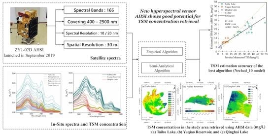
Total suspended matter concentration (C_TSM) is an important parameter in aquatic ecosystem studies. Compared with multispectral satellite images, the Advanced Hyperspectral Imager (AHSI) carried by the ZY1-02D satellite can capture finer spectral features, and the potential for C_TSM retrieval is enormous. In this study, we selected seven typical Chinese inland water bodies as the study areas, and recalibrated and validated 11 empirical models and two semi-analytical models for C_TSM retrieval using the AHSI data. The results showed that the semi-analytical algorithm based on the 697 nm AHSI-band achieved the highest retrieval accuracy (R² = 0.88, average unbiased relative error = 34.43%). This is because the remote sensing reflectance at 697 nm was strongly influenced by C_TSM, and the AHSI image spectra were in good agreement with the in-situ spectra. Although further validation is still needed in highly turbid waters, this study shows that AHSI images from the ZY1-02D satellite are well suited for C_TSM retrieval in inland waters.

1. Introduction

More than 40% of the world’s population lives in coastal areas or along rivers and lakes [1], while the water quality of numerous water bodies has deteriorated in recent decades owing to intensified human activities. In particular, the widespread problem of microplastics in water bodies poses a potential threat to the health of people [2]. Inland waters are more fragile than marine ecosystems because of their more confined nature and lower ecological stability [3]. Total suspended matter is a widely used water quality parameter in aquatic environmental studies, which mainly refers to solids suspended in water bodies, including inorganic substances that are insoluble in water, organic substances, sediment, and microorganisms [4]. The presence of suspended matter alters the distribution of light intensity in the water body, affecting the growth of aquatic vegetation and thus the distribution of primary productivity and biomass in the water body [5].

Water quality monitoring based on in-situ measurements usually only represents the status of stations. It is costly and difficult to provide continuous large-scale monitoring over time. With the rapid development of remote sensing technology, large-scale and long time-series remote sensing products are increasingly being used [6,7]. Satellite image-based C_TSM retrieval can effectively overcome the shortcomings of traditional methods and is being increasingly used for reflecting the water quality of the water body [8,9,10]. At present, the main methods for estimating C_TSM utilizing remote sensing products are empirical [7,11,12,13,14], semi-analytical [15], and analytical [16]. Among them, empirical methods, with advantages of simple steps and fast processing, are mainly based on linear regression of a single band or a combination of bands [5,8,9,17,18]. However, the applicability of empirical models varies widely across water bodies [19], and it is difficult to find a general empirical model that can be applied to most water bodies. The semi-analytical method can avoid the shortcomings of empirical models to a certain extent and has better applicability to different water bodies. Nechad [15] developed a single-band semi-analytic C_TSM retrieval model based on a bio-optical model and provided calibration results for MODIS, MERIS, and SeaWiFS sensors. This method was later successfully applied to Landsat8-OLI and Sentinel2-MSI sensors [20] with good generalizability. The analytical method mainly simulates the light field distribution of the water body based on the radiative transfer model, and uses the relationship between the water color signal and the spectral properties of the water body to estimate the content of each component of the corresponding water body. The physical meaning of this process is clearer and more general in space and time, but it is less commonly used in practical applications because the theoretical application of absorption and scattering in different water bodies is still immature and the arithmetic process is relatively more complicated [21].

The spatial, temporal, spectral, and radiometric resolutions of the satellite sensors (

Table 1. Specifications of commonly used satellite-based hyperspectral sensors [27,28,29].

Sensor	Spectral Range (nm)	Spectral Bands	Spectral Resolution (nm)	Spatial Resolution (m)	Swath Width (km)
Hyperion	357–2576	220	10	30	7.5
PROBA-CHRIS	415–1050	19/63	34/17	17/36	14
HICO	360–1080	128	5.7	90	192
PACE-OCI	342.5–887.5	-	5	1000	2663
HJ-1A HSI	450–950	115	5	100	50
GF5 AHSI	400–2500	330	5/10	30	60
ZY1-02D AHSI	400–2500	166	10/20	30	60

) can affect their capabilities in water-color remote sensing [22]. Different types of sensors have different limitations for estimating total suspended matter concentrations [19]. First, multispectral sensors with broadbands, such as Landsat8 OLI and Sentinel-2 MSI, generally have relatively high spatial resolution, but with only a few numbers of bands. Second, multi-spectral sensors with narrow widths, (e.g., Sentinel-3 OLCI and MERIS) can capture the spectral characteristics of suspended matter more accurately. However, the spatial resolution of this type of data is usually very low (300–1200 m), making it hard to be applied to small- and medium-sized water bodies. In comparison, hyperspectral data (e.g., GF-5 AHSI and ZY1-02D AHSI) have relatively spatial resolution (i.e., 30 m) and abundant narrow bands, thereby serving as a suitable data source for total suspended matter monitoring of inland waters [23,24].

China successfully launched the GF-5 satellite in May 2018. GF-5 carries the Advanced Hyperspectral Imager (AHSI), which is capable of acquiring images with 5 nm and 10 nm spectral resolution in the visible to near-infrared (VNIR) bands and short-wave infrared (SWIR) bands, respectively. The number of bands was 330, and its spatial resolution was 30 m, and the swath width was 60 km. Subsequently, the ZY1-02D satellite was successfully launched in September 2019, carrying the new-generation AHSI, which has the same spatial resolution and swath width as GF-5. However, to improve the signal-to-noise ratio of the data, the spectral resolution in the VNIR and SWIR bands of ZY1-02D AHSI was reduced to 10 nm and 20 nm [25], respectively. As a result, while maintaining wide swath and coverage capability, the signal-to-noise ratio (SNR) of the ZY1-02D AHSI sensor was improved compared with the GF-5 AHSI. The minimum SNR of the sensor under typical operating conditions exceeds 120, allowing for uninterrupted long strip imaging [26]. Therefore, ZY1-02D hyperspectral data have a high potential for application in the quantitative information extraction of inland water bodies.

The main purpose of this study is to test the capability of the ZY1-02D AHSI for total suspended matter retrieval in inland waters, and thereby identify the optimal model that can be applied to AHSI data of ZY1-02D. Section 2 describes the data and retrieval strategy, Section 3 the data processing methods and alternative models, and Section 4 the calibration and validation results of the selected model. An experimental discussion is presented in Section 5 and conclusions are drawn in Section 6.

2. Materials

2.1. R_rs and C_TSM Field Measurements

From May 2019 to July 2021, 9 field experiments were carried out in 7 inland lakes and reservoirs of China. Details of the study areas and measurement information are given in

Table 2. Study region, acquisition date, number of samplings (N), statistics of CTSM and $R_{rs}$.

No.	Study Region	Elevation(m)	Acquisition Date	N	CTSM (mg/L)			ZY1E Acquisition Date	${\mathit{R}}_{\mathit{r}\mathit{s}}\left({\mathbf{sr}}^{-1}\right)$
					Mean	Min.	Max.		Std (10−3)
1	Taihu Lake	4	1 May 2019	10	30.5	6.0	49.0	-	4.67
2	Baiyangdian Lake	5	21 May 2019	23	9.7	4.3	17.3	-	1.60
3	Guanting Reservoir	473	22 May 2019	18	10.9	5.5	33.0	-	2.07
4	Daheiting Reservoir	989	24 September 2019	10	5.7	3.7	7.5	-	0.63
5	Panjiakou Reservoir	172	24 September 2019	17	3.8	2.6	5.0	-	0.56
6	Yuqiao Reservoir	16	8 October 2019	19	18.3	7.3	29.0	-	6.42
7	Taihu Lake	4	6 September 2020	17	32.2	18.7	53.5	6 September 2020	2.90
8	Yuqiao Reservoir	16	8 November 2020	10	8.5	5.0	11.8	8 November 2020	1.49
9	Qinghai Lake	3260	27 July 2021	10	2.8	1.9	3.9	28 July 2021	1.41

. Specifically, 7 field experiments conducted in 2019 include a total of 97 sets that have C_TSM of 2.6–49 mg/L. In-situ data of these 97 sampling sites were used as calibration sets. Three field experiments conducted in 2020 and 2021 include 37 sampling sites in Taihu Lake, Yuqiao Reservoir, and Qinghai Lake, with C_TSM ranging from 1.9 to 53.5 mg/L. Field measurements at these 37 sampling sites were used as validation sets.

As one of the five major freshwater lakes in China, Taihu Lake has a water area of about 2338 km². Nevertheless, it is a typical shallow lake, with an average water depth of about 1.9 m [30]. Baiyangdian Lake is an important natural lake in northern China, and located in the middle of the Daqing River Basin. It has a water area of about 366 km² and an average depth of about 3.6 m. Qinghai Lake, the largest inland lake in China, is located in the northeastern part of the Tibetan Plateau, with an area of approximately 4553 km². Yuqiao Reservoir, also known as Cuiping Lake, is 15 km long from east to west and 5 km wide from north to south, with a total watershed area of approximately 2060 km² with a water depth of approximately 4.7 m [31]. Other reservoirs can be found in northern China, with water surface areas ranging from tens to hundreds of square kilometers, and their water quality is generally good. The locations and sample points of the 3 study areas which have AHSI concurrent images are shown in Figure 1.

The main indicators collected were C_TSM and in-situ spectra. C_TSM was measured by the drying and weighing method. After obtaining surface water samples in the field, the samples were brought back to the laboratory within 24 h. In the laboratory, water samples were filtered using a 0.45 µm pore size filter membrane and dried to a constant mass at 103–105 °C. Repeated drying, cooling, and weighing was done until the difference between two weighing results was less than or equal to 0.4 mg/L [32]. The sampling time and the statistical information of C_TSM are shown in Table 2. While collecting water samples, in-situ spectra were collected using an ASD Field Spec Pro spectrometer according to the above-water method [33].

Remote sensing reflectance spectra were calculated by measuring the reference plate radiance ($L_p\left(\lambda \right)$), sky radiance ($L_{sky}\lambda$), and water surface radiance ($L_u\lambda$). For $L_u\lambda$ measurements, the viewing zenith angle was 40° downward, and the azimuth angle was 135° away from the sun azimuth. The viewing zenith angle was 40° upward for $L_{sky}\lambda$ measurements, and the azimuth angle was the same as for $L_u\lambda$ measurements. The reference plate radiance was measured by aiming at the center of the reference plate vertically downward. For the water surface radiance measurements at each sampling site, we performed 10 replicate measurements and checked the results. Anomalous spectra caused by random solar flares may be present in the measured result. These anomalous results were discarded, and the remaining spectra were averaged.

The above-water remote sensing reflectance was calculated by the following equation:

$$R_{rs}=\frac{L_u\left(\lambda \right)-{\rho }_{sky}\left(\lambda \right)L_{sky}\left(\lambda \right)}{\pi L_p\left(\lambda \right)/{\rho }_p\left(\lambda \right)},$$

(1)

where ${\rho }_p$ is the standard panel reflectance calibrated in the laboratory and the ${\rho }_{sky}$ is the air–water interface skylight reflectance.

As shown in Table 2, a total of 134 sets of data were obtained, including $R_{rs}$ and C_TSM. Among them, 97 of the sampling points with earlier sampling times had no concurrent images, and they only had the in-situ measured $R_{rs}$ and C_TSM. So, they were used for the original calibration of the C_TSM estimation model. The in-situ measured $R_{rs}$ of these sampling points are shown in Figure 2.

In addition to this, there are 37 sampling points which have AHSI concurrent images and their locations are shown in Figure 1. The in-situ $R_{rs}$ and C_TSM of these points were used to validate the calibrated model. In-situ measured $R_{rs}$ for these sampling points are shown in Figure 3.

2.2. Concurrent ZY1-02D Image Acquisition

The ZY1-02D satellite AHSI images were selected based on the field measurement time ±1 d, and stable meteorological conditions. Specifically, all in-situ measurements of Taihu Lake and Yuqiao Reservoir were measured within 3 h of the ZY1-02D satellite overpasses. Images of Qinghai Lake were acquired 1 day after the in-situ measurements. Since Qinghai Lake is a deep lake (average water depth of 21 m), and the meteorological condition is stable during the in-situ measurements and satellite image acquisition, the C_TSM is relatively stable in this study region. Therefore, the in-situ measurements in Qinghai Lake are counted as match-ups despite the 1-day difference between them. All images were acquired around 11:00 a.m. local time with less than 10% cloud coverage. To match the image $R_{rs}$ with in-situ $R_{rs}$, a 3 × 3 pixel window centered at the posistion of the sampling points was used. If the coefficient of variation (i.e., standard deviation/mean) was less than 0.40 in the window, the central pixel of the 3 × 3 pixel window was selected as a match-up [34].

AHSI concurrent images $R_{rs}$ of 37 validation points in Taihu Lake, Yuqiao Reservoir and Qinghai Lake were used to verify the accuracy of AHSI image retrieval C_TSM.

3. Methods

3.1. AHSI Band R_rs Simulations

For hyperspectral sensors with narrow band widths, the spectral response function (SRF) in each band is usually described using the Gaussian function [35,36] as follows:

$$f_i\left(\lambda \right)=\exp \left[-4ln2{\left(\frac{\lambda -{\lambda }_i}{\mathsf{\Delta }{\lambda }_i}\right)}^2\right]$$

(2)

where ${\lambda }_i$ is the central wavelength of each band, $\mathsf{\Delta }{\lambda }_i$ is the FWHM of each band. For AHSI sensors, VNIR and SWIR have FWHMs of 8.76 and 16.26 nm, respectively. Based on SRF, the in-situ $R_{rs}$ can be converted to AHSI band-equivalent $R_{rs}$ using the following equation:

$$R_{rs}^m\left(B_i\right)=\frac{{{\displaystyle \int }}_{{\lambda }_{min}}^{{\lambda }_{max}}{R}_{rs}^m\left(\lambda \right)f_i\left(\lambda \right)d\lambda }{{{\displaystyle \int }}_{{\lambda }_{min}}^{{\lambda }_{max}}{f}_i\left(\lambda \right)d\lambda }$$

(3)

where $f_i\left(\lambda \right)$ is the SRF of ith band, ${\lambda }_{max}$ and ${\lambda }_{min}$ represent the maximum and minimum wavelengths in this band, respectively. According to Equation (3), the conversion of in-situ $R_{rs}$ to AHSI-band $R_{rs}$ can be achieved.

3.2. C_TSM Model Development Using the In-Situ Dataset

Two methods are usually used to estimate C_TSM using remote sensing reflectance: 1. The relationship between $R_{rs}$ and C_TSM, which is an empirical algorithm. They are classified into single-band and multi-band algorithms; 2. The backscatter coefficient ($b_{bp}$) can be estimated by remote sensing reflectance, and then the relationship between $b_{bp}$ and C_TSM can be established, which is a semi-analytical method. The typical models of the different algorithms are presented below.

3.2.1. Empirical Algorithm

• Single-band empirical models

As the C_TSM in water increased, the reflectance of the water in the VNIR band also increased gradually. The reflection peaks of the spectra of water with different C_TSM appeared at 580–700 nm. Among the related studies, red-band retrieval has been the most frequently used [7,8,9]. However, when the C_TSM is excessively high, the reflectance of the visible region tends to saturate [37]. To avoid this phenomenon, there are models that change the retrieval wavelength to the NIR band [14,17].

• Multi-band empirical models

With increasing C_TSM in water, the wavelength of the reflection peak shifts towards the long-wave direction. Therefore, the band-ratio model can be established using the reflection peak of the red-NIR bands and the low reflectance of the blue-green bands. Because of the strong absorption at 940 nm and 1130 nm, the choice of reflection peak wavelength is mostly <850 nm, such as in Doxaran_02 [37], He_13 [13], and Hou_17 [38].

By constructing spectral feature parameters, the absorption and reflection characteristics of the spectral profile can be effectively highlighted for accurate C_TSM retrieval. Spectral characteristic parameters are available in various forms. One of the typical combinations is the spectral absorption characteristics obtained by the spectral absorption index or the spectral envelope method, also known as the baseline model, such as in Kuster_16 [39] and Liu_18 [40]. In addition, the three-band model (Zhang_10 [10]) and the normalized model (Zhang_10_1 [41]) have also been developed and are applicable for different water bodies.

All the empirical models and their utilized bands or spectral indices are listed in

Table 3. Wavelength or spectral combinations used in empirical methods.

Model Type	Model Name	Band or Spectral Index	Source
Single-band model	Zhang_09	$R_{rs}\left(774\right)$	[17]
	Petus_10	$R_{rs}\left(645\right)$	[9]
	Zhang_14	$R_{rs}\left(705\right)$	[14]
Multi-bands models	Doxaran_02	$R_{rs}\left(816\right)/R_{rs}\left(551\right)$	[37]
	He_13	$R_{rs}\left(748\right)/R_{rs}\left(490\right)$	[13]
	Hou_17	$R_{rs}\left(645\right)/R_{rs}\left(551\right)$	[38]
	Kuster_16_1	$R_{max}\left(700-720\right)-\left[R_{rs}\left(645\right)+R_{rs}\left(774\right)\right]/2$	[39]
	Kuster_16_2	$R_{rs}\left(810\right)-\left[R_{rs}\left(774\right)+R_{rs}\left(842\right)\right]/2$	[39]
	Liu_18	$\mathrm{SAI}=\frac{d\times R_{rs}\left(490\right)+\left(1-d\right)\times R_{rs}\left(745\right)}{R_{rs}\left(551\right)},$ $d=\frac{551-490}{745-490}$	[40]
	Zhang_10	$X1=R_{rs}\left(560\right)+R_{rs}\left(645\right);X2=R_{rs}\left(490\right)/R_{rs}\left(560\right)$	[10]
	Zhang_10_1	$\frac{R_{rs}\left(490\right)-R_{rs}\left(645\right)}{R_{rs}\left(551\right)+R_{rs}\left(551\right)}$	[41]

.

3.2.2. Semi-Analytical Algorithm

The backscattering coefficient ($b_{bp}$) at specific wavelengths is closely linked to C_TSM [15]. At present, the $b_{bp}$ of water bodies is mostly estimated based on semi-analytical methods, which are more stable than empirical models owing to the incorporation of physical-optical principles [42]. Therefore, the method of estimating C_TSM based on $b_{bp}$ has higher stability and applicability. In this study, we consider 2 types of semi-analytic algorithms: QAA-based and Nechad C_TSM retrieval methods. They were applied to the ZY1-02D AHSI data, and the accuracies were evaluated.

• QAA-based $C_{TSM}$ retrieval method

There are two main steps in this method: 1. Calculate $b_{bp}$ using the QAA; and 2. build an empirical model between $b_{bp}$ and C_TSM.

In this study, we calculated $b_{bp}$ using two original QAA models (QAA_V5 and QAA_V6) and three improved models (Le_09 [43], Mishra_14 [44], and Jiang_21 [45]). Among them, the reference wavelength of QAA_V5 is 555 nm [46], whereas the reference wavelength of QAA_V6 is shifted to 670 nm to adapt to highly turbid or eutrophic waters [47]. The steps involved in the two types of QAA methods are listed in

Table 4. Steps of the two original types of quasi-analytical algorithm (QAA) method.

Step	Property	$\mathbf{QAA}\_\mathbf{V}5 ({\mathit{\lambda }}_0 = 555)$	$\mathbf{QAA}\_\mathbf{V}6 ({\mathit{\lambda }}_0 = 670)$
1	$r_{rs}\left(\lambda \right)$	$r_{rs}\left(\lambda \right)=R_{rs}\left(\lambda \right)/\left(0.52+1.7R_{rs}\left(\lambda \right)\right)$
2	$u\left(\lambda \right)$	$u\left(\lambda \right)=\frac{-0.089+\sqrt{{0.089}^2+4\times 0.125r_{rs}\left(\lambda \right)}}{2*0.125}$
3	$a\left({\lambda }_0\right)$	$$\begin{gathered} a\left({\lambda }_0\right) \\ =a_{\omega }\left({\lambda }_0\right)+{10}^{-1.146-1.366\chi -0.469{\chi }^2} \end{gathered}$$ $\chi =log\left(\frac{r_{rs}\left(443\right)+r_{rs}\left(490\right)}{r_{rs}\left({\lambda }_0\right)+5\frac{r_{rs}\left(667\right)}{r_{rs}\left(490\right)}{r}_{rs}\left(667\right)}\right)$	$\mathrm{If}{R}_{rs}\left(\lambda \right)<0.0015s{r}^{-1}$: Same as QAA_V5. $$\begin{gathered} \mathrm{Else} a\left({\lambda }_0\right)=a_{\omega }\left({\lambda }_0\right)+ \\ 0.39{\left(\frac{R_{rs}\left(670\right)}{R_{rs}\left(443\right)+R_{rs}\left(490\right)}\right)}^{1.14} \end{gathered}$$
4	$b_{bp}\left({\lambda }_0\right)$	$b_{bp}\left({\lambda }_0\right)=\frac{u\left({\lambda }_0\right)\times a\left({\lambda }_0\right)}{1-u\left({\lambda }_0\right)}-b_{bw}\left(670\right)$
5	$\mathsf{\eta }$	$\eta =2.0\left(1-1.2exp\left(-0.9\frac{r_{rs}\left(443\right)}{r_{rs}\left(555\right)}\right)\right)$
6	$b_{bp}\left(\lambda \right)$	$b_{bp}\left(\lambda \right)=b_{bp}\left({\lambda }_0\right){\left(\frac{{\lambda }_0}{\lambda }\right)}^{\eta }$

. In addition, other scholars have modified the QAA model to adapt to inland water bodies with complex optical properties, such as adjusting the empirical formula [43,44,48] and developing a new semi-analytical algorithm to replace the original empirical algorithm part [49].

In Table 4, $r_{rs}\left(\lambda \right)$ is the remote sensing reflectance below the water surface, $a\left(\lambda \right)$ is the total absorption coefficient, and $b_{bw}\left(\lambda \right)$ is the backward scattering coefficient of pure water. The major difference between QAA_V5 and QAA_V6 is that $a\left(\lambda \right)$ is calculated differently. The $b_{bp}\left(\lambda \right)$ calculated by the algorithm was then linked to the C_TSM.

Linear models were used to retrieve the C_TSM because of the linear relationship between $b_{bp}$ and C_TSM:

$$C_{TSM}=\mathrm{a}*b_{bp}+b{,}_{ }$$

(4)

where a and b are the coefficients of the linear model obtained by calibrating the calibration dataset.

Because the Jiang_21 model was obtained from a calibration dataset with a wider C_TSM range [45], the origin linear model was used directly in this study and was not recalibrated.

• Nechad retrieval method

Nechad_10 retrieval model is a simplified model based on reflectance, which links single-band reflectance to TSM concentration. It has been successfully applied to water-color satellite sensors such as SeaWiFS and MODIS [15], its main formulas are as follows:

$$C_{TSM}=\frac{\mathsf{\pi }{A}^{\rho }\left(\lambda \right)R_{rs}\left(\lambda \right)}{1-\mathsf{\pi }{R}_{rs}\left(\lambda \right)/C^{\rho }\left(\lambda \right)}+B^{\rho }\left(\lambda \right),$$

(5)

$$A^{\rho }=A/\gamma$$

(6)

$$C^{\rho }=\gamma C/(1+C)$$

(7)

$$\gamma =\pi \mathcal{R}{f}^{‘}/Q\approx 0.216,$$

(8)

where $A=a_{np}/b_{bp}^{*}$, $a_{np}$ represents the non-particulate absorption and $b_{bp}^{*}$ represents the constant TSM-specific particulate backscatter. $A^{\rho }$ and $B^{\rho }$ were obtained by nonlinear fitting and reparametrized based on the calibration dataset used in this study. $\mathrm{C}=b_{bp}^{*}/a_p^{*},$ $a_p^{*}$ represents the constant TSM-specific particulate absorption coefficient, which is determined by the IOPs and is independent of $R_{rs}$. therefore, the Nechad rated $C^{\rho }$ values were used directly [15].

3.2.3. Calibration and Validation

First, the parameters of the empirical and semi-analytical models were calibrated based on the in-situ $R_{rs}$ and in-situ C_TSM from 97 calibration datasets. Second, the calibrated models were validated using in-situ $R_{rs}$ and in-situ C_TSM from 37 validation datasets. Three indicators, i.e., the coefficient of determination (R²), root mean square error (RMSE), and average unbiased relative error (AURE), were used for accuracy analysis and were calculated as follows:

$$R^2=1-\frac{{{\displaystyle \sum }}_{i=1}^n{\left(y_i-\widehat{y_i}\right)}^2}{{{\displaystyle \sum }}_{i=1}^n{\left(y_i-\overline{y}\right)}^2},$$

(9)

$$\mathrm{RMSE}=\sqrt{\frac{1}{n}{{\displaystyle \sum }}_{i=1}^n{\left(y_i-\widehat{y_i}\right)}^2, \mathrm{and}}$$

(10)

$$\mathrm{AURE}=\frac{1}{n}\times {{\displaystyle \sum }}_{i=1}^n\frac{\left|y_i-\widehat{y_i}\right|}{0.5*\left(y_i+\widehat{y_i}\right)}\times 100\%,$$

(11)

where n is the number of samples, $\widehat{y_i}$ is the model estimated value, $y_i$ is the in-situ measurement value, and $\overline{y}$ is the mean value of the in-situ measurements.

3.3. C_TSM Retrieval Based on AHSI Images

After testing the empirical and semi-analytical models based on in-situ data, to retrieve the C_TSM from AHSI images, we first performed atmospheric correction of the images and extracted the water region. Then, the best empirical and semi-analytical models were applied to the AHSI images, and finally the accuracy evaluation of the image retrieval results was achieved by the in-situ measured C_TSM.

3.3.1. AHSI Image Preprocessing

Pre-processing of the AHSI images is a prerequisite for estimating the total suspended matter concentration, including atmospheric correction and water body extent extraction. First, the Digital Number (DN) values were converted into apparent radiances using radiometric calibration coefficients. Second, atmospheric correction was performed using the FLAASH atmospheric correction tool. In the FLAASH module, most of the parameters were set according to the official documentation [50]. For the ZY1-02D hyperspectral data, the sensor altitude was set to 778 km, and we chose the 940 nm water vapor retrieval band.

Using the ZY1-02D surface reflectance ($\rho$) images retrieved from FLAASH, the automated water extraction index (AWEI) was calculated as follows [51]:

$$AWE{I}_{nsh}=4*\frac{{\rho }_{559}-{\rho }_{1610}}{0.25*{\rho }_{842}+2.75*{\rho }_{2183}}.$$

(12)

The delineation of water bodies was then achieved using the OTSU method [52] based on the AWEI. To correct the skylight effect and retrieve remote sensing reflectance from surface reflectance images, an image-based method for remote sensing reflectance estimation [53] was applied as follows:

$$R_{rs}\left(\lambda \right)=\frac{\rho \left(\lambda \right)-\min \left({\rho }_{NIR}:{\rho }_{SWIR}\right)}{\pi },$$

(13)

where $R_{rs}\left(\lambda \right)$ represents the remote sensing reflectance of the image; $\rho \left(\lambda \right)$ represents the surface reflectance; and $\min \left({\rho }_{NIR}:{\rho }_{SWIR}\right)$ represents the minimum surface reflectance in the NIR and SWIR bands, respectively, where ${\rho }_{NIR}$ and ${\rho }_{SWIR}$ use the mean $\rho$ in the AHSI bands of 720–730 nm and 1530–1630 nm, respectively.

3.3.2. AHSI-Retrieved C_TSM Accuracy Assessment

After the consistency check between AHSI image $R_{rs}$ and in-situ $R_{rs}$, the models were validated using the AHSI image-derived $R_{rs}$ from the validation dataset. Then, models with high accuracy were applied to AHSI images. It should be noted that in-situ $R_{rs}$ was converted to band-equivalent $R_{rs}$ in the AHSI bands by the method in Section 3.1.

For the accuracy analysis of the satellite-ground spectral consistency, the spectral angle cosine was calculated as follows:

$$\cos \mathsf{\alpha }=\frac{{{\displaystyle \sum }}_{i=1}^n{y}_j^i{\widehat{y}}_j^i}{\sqrt{{{\displaystyle \sum }}_{i=1}^n{\left(y_j^i\right)}^2{{\displaystyle \sum }}_{i=1}^n{\left({\widehat{y}}_j^i\right)}^2}},$$

(14)

where n is the number of samples and $y_j^i$ and ${\widehat{y}}_j^i$ are the in-situ $R_{rs}$ and AHSI image $R_{rs}$ of samples i and band j, respectively.

Based on the pre-processed AHSI images, C_TSM was retrieved using the best empirical and semi-analytical method and 37 matched points were used to evaluate the accuracy of the image retrieval C_TSM using R², RMSE, and AURE.

4. Results

4.1. Accuracy Assessment of ZY1-02D Image Atmospheric Correction

The accuracy of the image-derived remote sensing reflectance affected the accuracy of the estimated C_TSM. Therefore, the accuracy evaluation of ZY1-02D image-derived $R_{rs}$ was conducted for the main bands utilized in the C_TSM retrieval models using R² and AURE. The results are shown in

Table 5. Accuracy analysis of the ZY1-02D image-derived $R_{rs}$.

ZY1-02D Bands (nm)	${\mathit{R}}_{\mathit{r}\mathit{s}}\left(490\right)$	${\mathit{R}}_{\mathit{r}\mathit{s}}\left(551\right)$	${\mathit{R}}_{\mathit{r}\mathit{s}}\left(560\right)$	${\mathit{R}}_{\mathit{r}\mathit{s}}\left(645\right)$	${\mathit{R}}_{\mathit{r}\mathit{s}}\left(697\right)$	${\mathit{R}}_{\mathit{r}\mathit{s}}\left(748\right)$	${\mathit{R}}_{\mathit{r}\mathit{s}}\left(774\right)$	${\mathit{R}}_{\mathit{r}\mathit{s}}\left(800\right)$	${\mathit{R}}_{\mathit{r}\mathit{s}}\left(816\right)$	${\mathit{R}}_{\mathit{r}\mathit{s}}\left(842\right)$
R2	0.68	0.87	0.88	0.95	0.96	0.52	0.53	0.73	0.71	0.29
AURE (%)	32.60	18.84	18.99	36.35	30.17	109.21	113.05	77.29	81.21	134.37

.

Among the major bands utilized by the models, 551 nm had the lowest AURE of 18.84%, which was the band with the highest agreement between image remote sensing reflectance and in-situ remote sensing reflectance. As can be seen from Figure 2 and Figure 3, the energies of 551 and 560 nm were higher than that of other wavelengths; therefore, they were relatively less affected by noise. Similarly, the red bands of 645–700 nm were also relatively high in energy and received relatively little noise impact, with AUREs of approximately 30%. It is known from the remote sensing principle that the shorter the wavelength, the weaker the penetration ability, while the atmosphere has a strong scattering effect in the blue band. Therefore, the consistency of the 490 nm satellite spectrum was poor compared with the red and green bands; however, the AURE was still controlled at 32.60%. The NIR band after 750 nm was lower in energy, and there was only a very small reflection peak at 800 nm, which was more affected by noise; therefore, its relative error was also relatively high.

Subsequently, the spectral angle cosine was calculated separately for the satellite-ground spectra of each study area to determine the spectral consistency in different study areas, as shown in

Table 6. Spectral angle cosine of validation datasets. SD—standard deviation.

Study Area	Spectral Angle Cosine
	Mean	Min.	Max.	SD
Taihu Lake	0.991	0.949	0.998	0.013
Yuqiao Reservoir	0.993	0.988	0.998	0.003
Qinghai Lake	0.909	0.838	0.955	0.038

.

The mean values of the spectral angle cosine in all three regions were >0.9, indicating that the AHSI image spectra were in good agreement with the in-situ spectra.

4.2. C_TSM Estimation from In-Situ Measurements by Empirical Models

First, we tested 11 empirical models, which were divided into two categories: Single-band and multi-bands models. Among the empirical models, the selected bands for each model were adapted according to the AHSI bands. For the model calibration, we compared the model equation of the original literature, and four types of fitting functions: linear, exponential, logarithmic, and power functions. The model with the highest R² was chosen as the best fitting model. In addition, the fitting function should be monotonous to avoid estimation anomalies. The calibration and validation results of the models are presented in

Table 7. Calibration and validation results of empirical models based on in-situ $R_{rs}$. Optimal results in each type of model are shown in bold.

Model Name	Calibration Dataset		Validation Dataset
	Calibrated Model	R2	R2	RMSE	AURE (%)
Zhang_09	$1056.1x^{0.71}$	0.85	0.93	4.36	21.48
Petus_10	$1405.8x+1.41$	0.69	0.91	4.48	23.32
Zhang_14	$523.7x^{0.71}$	0.86	0.92	5.29	21.68
Doxaran_02	$e^{6.76x+1.19}$	0.52	0.56	11.38	48.22
He_13	$51.98x+0.47$	0.52	0.42	12.84	68.76
Hou_17	$1.50e^{3.1x}$	0.29	0.49	13.25	52.60
Kuster_16_1	$3973.4x+3.94$	0.80	0.85	6.62	26.98
Kuster_16_2	$10453x+5.03$	0.83	0.92	4.41	28.45
Liu_18	${10}^{3.89*x1+0.072}$	0.74	0.03	19.81	75.90
Zhang_10	${10}^{1.16+17.33*x1-0.97*x2}$	0.44	0.89	4.96	19.08
Zhang_10_1	${10}^{0.0156x^3-1.17x+0.97}$	0.43	0.34	15.32	70.57

and Figure 4.

In the empirical models, the calibration of the single-band model based on the NIR band after 700 nm was generally good, with R² > 0.85. Among the multi-band models, the baseline model was generally better; the Kuster_16_2 model (R² = 0.83) was the best calibrated multiband model. The results of the other multiband models were generally lower.

From the validation results, the Zhang_10 ratio model had the best validation results, with the lowest AURE of 19.08%. The single-band model was also generally good, with a validation AURE of approximately 20%. Among the multi-band models, Kuster_16 showed better results on the validation set, with AURE < 30%, whereas the validation results of the Liu_18 model were poor and not applicable to the estimation of C_TSM in inland waters. The ratio model still performed poorly in the validation set. Determining the optimal empirical model applicable to AHSI images requires further validation.

4.3. C_TSM Estimation from In-Situ Measurements by Semi-Analytical Models

$b_{bp}$ values were calculated using QAA and its improved models for indirect estimation of the total suspended matter concentration. The Jiang_21 model established the relationship between the $b_{bp}$ and C_TSM over a wider range of C_TSM. Therefore, the parameters were not re-rated. Other models re-rated the relationship between $b_{bp}$ and C_TSM based on calibrated datasets to enable the estimation of C_TSM. The Nechad_10 model showed the best calibration results at 697 nm with parameters $A^{\rho }$ and $B^{\rho }$: 934.09 (g/m³) and 4.39 (g/m³), respectively. C_TSM was then retrieved based on image-derived $R_{rs}$ using various semi-analytical models. The calibration and validation results of C_TSM estimated on the ZY1-02D match-ups are shown in

Table 8. Calibration and validation results of semi-analytical models based on in-situ $R_{rs}$. Optimal results are shown in bold.

Model Name.	Calibrated TSM Model	Calibration Dataset R2	Validation Dataset
			R2	RMSE	AURE (%)
QAA_V5	$145.83*b_{bp}\left(551\right)+1.44$	0.68	0.92	4.76	25.96
QAA_V6	$116.92*b_{bp}\left(662\right)+2.83$	0.71	0.92	6.55	33.00
Le_09	$97.4*b_{bp}\left(714\right)+3.08$	0.85	0.87	7.00	32.84
Mishra_14	$76.323*b_{bp}\left(705\right)+2.89$	0.85	0.88	7.24	35.44
Jiang_21	$if R_{rs}\left(490\right)>R_{rs}\left(560\right):$ $94.607*b_{bp}\left(705\right)$ $else: 114.012*b_{bp}\left(665\right)$	0.82	0.87	8.45	59.38
Nechad_10	$\frac{934.09R_{rs}\left(697\right)}{1-R_{rs}\left(697\right)/0.05911}+4.39$	0.77	0.94	4.22	28.92

and Figure 5.

In the QAA-based C_TSM retrieval method, even though the Le_09 and Mishra_14 models achieved the highest R² in the calibration dataset, QAA_v5 achieved the optimal performance in the validation dataset. This was mainly due to the utilization of the 551 nm band, for which the image-derived $R_{rs}$ was reasonably accurate.

The accuracy of the Nechad_10 model gradually improved as the wavelength shifted toward the long wave direction, and the highest validation accuracy was achieved at 697 nm. Generally, the difference in the C_TSM estimation accuracy between the two types of semi-analytical models was insignificant.

4.4. C_TSM Estimation from AHSI Images

To investigate the applicability of different models to satellite images, optimal single-band and multi-band empirical models, the QAA_V5 based model, and Nechad_10 (697 nm) model were applied to the image-derived $R_{rs}$ of match-ups, and the validation accuracy results are shown in

Table 9. Validation results of the best C_TSM retrieval models based on the AHSI images $R_{rs}$. Optimal results are shown in bold.

Model Name	R2	RMSE	AURE (%)
Zhang_09	0.61	10.16	58.39
Kuster_16_2	0.87	6.34	39.27
Zhang_10	0.87	7.40	37.84
QAA_V5	0.87	6.31	40.34
Nechad_10(697)	0.88	6.66	34.43

. The best results are shown in Figure 6.

Based on the Nechad_10 (697 nm) model, the total suspended matter concentration distributions were produced for the three study areas (Figure 7). The overall trend of C_TSM in Taihu Lake decreased from northwest to southeast, while most rivers entering the lake are located along the northwestern coast of Taihu Lake. The confluence of the rivers increases the movement of the lake, resulting in higher C_TSM at the northwest of Taihu Lake, while the central and eastern parts are less affected by this trend [41]. The C_TSM in Yuqiao Reservoir did not vary considerably, with low C_TSM values in the center of the reservoir and high C_TSM values along the northern coast due to human activities [31]. The highest C_TSM existed in the eastern part of the reservoir, where the Lin River entered the lake, reaching >13 mg/L. Due to the limited coverage of the AHSI image, only the C_TSM in the central region of Qinghai Lake was estimated. The overall C_TSM in Qinghai Lake was very low, mostly approximately 3 mg/L. The suspended matter concentration was low in the middle of the lake, and showed an increasing trend from the center of the lake to the lake shore.

5. Discussion

5.1. Evaluation of C_TSM Estimation Methods for AHSI Images

Based on calibration and validation results (Table 9), the final model chosen in this study was the Nechad_10(697) model, which achieved the highest accuracy among all the Nechad_10 models with different bands. As revealed by the in-situ C_TSM estimation results in Table 8, the AURE brought by the Nechad_10(697) is 28.92% (Figure 5b). Considering the uncertainties in AHSI image-derived $R_{rs}$, we compared the image-derived C_TSM with that estimated based on in-situ $R_{rs}$. The corresponding results are shown in Figure 8, which suggests the error brought by the image-derived $R_{rs}$ uncertainty is 13.64%.

In addition, Figure 5b demonstrates the accuracy of C_TSM retrieval based on in-situ measure $R_{rs}$. Most of the validation points are distributed along the 1:1 line. $B^{\rho }$ in the Nechad_10(697) model is represented as the intercept of the fitting line, as C_TSM is equal to $B^{\rho }$ when $R_{rs}$ is zero. Therefore, the retrieved C_TSM is more sensitive to the parameter $B^{\rho }$ when the C_TSM is low. This results in the Nechad_10(697) model overestimating the C_TSM for Qinghai Lake as its C_TSM is generally lower than $B^{\rho }$, but a good retrieval for Yuqiao Reservoir and Taihu Lake. Therefore, the Nechad_10(697) model may bring relatively large errors for C_TSM retrieval in clear water bodies.

The C_TSM retrieval results of AHSI images showed an overall underestimation in the Taihu Lake region. According to the studies of Doxaran et al. [37] and Petus et al. [9], spectral saturation is more likely to occur when using wavelengths less than 600 nm to estimate C_TSM in regions with greater than 100 mg/L. However, the wavelengths and C_TSM chosen in this manuscript are not in this range. The high accuracy of image remote sensing reflectance is a prerequisite for accurate estimation of C_TSM. In the experiment, the AURE between the in-situ $R_{rs}$ and the AHSI image $R_{rs}$ at 697 nm reached 29.17% (Figure 9). When these two types of data were applied to TSM concentration estimation, it caused a 13.64% difference in the AURE of the C_TSM retrieval results. Based on the scatterplot of the spectrum at 697 nm, the underestimation is more likely due to the AHSI image’s uncertainties in atmospheric correction.

Overall, the Nechad_10 (697 nm) model provided the best prediction for AHSI images in the validation of Taihu Lake, Yuqiao Reservoir, and Qinghai Lake. However, during the model calibration and validation, most sampling sites had a C_TSM of less than 50 mg/L. Thus, the calibrated model parameters may not be applicable in regions with higher C_TSM. Although these sampling sites were located in lakes and reservoirs of varying sizes in China, the representativeness of the sampling areas is still limited. For example, the salt lakes in the Qinghai-Tibet Plateau or the lakes in the Mongolian Plateau were not included [54]. Studies have shown that saline lakes tend to have a higher C_TSM than freshwater lakes [55]. Saline lakes have longer water exchange times, and their absorption characteristics may be significantly altered in the process of microbial degradation. Therefore, retrieval models based on freshwater lakes may not be applicable in these areas. To sum up, when applying AHSI images to retrieve C_TSM, the Nechad model may be unable to achieve optimal performance in all inland waterbodies. More in-situ measurements are needed for further development of the C_TSM retrieval model to be applied on ZY1-02D AHSI images.

5.2. Comparison of C_TSM Retrieval with Multispectral Sensors

To verify that AHSI has advantages for C_TSM retrieval compared with multispectral sensors, a comparison was made with estimated C_TSM based on band $R_{rs}$ of Landsat-8 OLI, Sentinel-2 MSI, and Sentinel-3 OLCI. Since no images of Landsat-8, Sentinel-2, or Sentinel-3 were acquired for the study areas on the same date of the ZY1-02D overpasses, this comparison was conducted using in-situ measured $R_{rs}$.

First, band $R_{rs}$ of the Landsat-8 OLI, Sentinel-2 MSI, and Sentinel-3 OLCI were simulated using their respective SRFs and the in-situ measured $R_{rs}$. Second, parameters in the optimal empirical and semi-analytical models (i.e., the Zhang_09 model and the Nechad_10 model) were recalibrated based on the calibration dataset of the simulated band $R_{rs}$. The same as in Section 4.2 and Section 4.3, the 97 and 37 datasets were used for model calibration and validation, respectively. Third, simulated bands of $R_{rs}$ of the 37 datasets were then respectively applied to Zhang_09 and Nechad_10 models for C_TSM estimation. Finally, accuracy analysis was conducted for estimated C_TSM using the simulated band $R_{rs}$ of these multispectral sensors, and then compared with the AHSI results in Table 7 and Table 8.

In terms of the Zhang_09 model, Sentinel-2 MSI acquired the best performance among the three multispectral sensors. Specifically, the 783 nm band of MSI was used and achieved an AURE of 21.58%, which is slightly higher than the AURE of AHSI (21.48%). For the Nechad_10 models established on band $R_{rs}$ of the multispectral sensors, the highest validation accuracy was also obtained by Sentinel-2 MSI with an AURE of 31.17%, which is also greater than that of AHSI (28.92%). This indicates that the AHSI’s narrow bands can help to improve the accuracy of C_TSM retrieval models.

6. Conclusions

The new-generation hyperspectral imaging spectrometer AHSI onboard the ZY1-02D satellite has continuous narrow spectral bands of 400–2500 nm, and can capture fine spectral features, thereby showing great potential for inland water C_TSM retrieval. In this study, we recalibrated 13 widely used empirical and semi-analytical C_TSM retrieval models using in-situ AHSI equivalent spectra of six typical inland water bodies in China. Validations based on in-situ spectra showed that the Zhang_10 model in the empirical model achieved the lowest AURE, (i.e., 19.08%). Two semi-analytical models established with the green and red bands, the QAA_V5-based model and the Nechad_10(697) model, had similar accuracy with AUREs of 25.96% and 28.92%, respectively. In terms of the validation based on the AHSI image-derived $R_{rs}$ of 36 match-ups, Nechad_10(697) achieved the best retrieval accuracy (AURE of 34.43%). This is owing to the robustness of the model, as well as the highly accurate AHSI band $R_{rs}$ at 697 nm.

Overall, the spectral and spatial resolution of ZY1-02D AHSI images makes it a useful data source for C_TSM retrieval of inland water bodies. With the advancement of atmospheric correction accuracy and model optimization based on a larger range of in-situ data, the accuracy of C_TSM retrieval based on ZY1-02D AHSI images will be further improved.

References

- Sloggett, D.; Srokosz, M.; Aiken, J.; Boxall, S. Operational Uses of Ocean Colour Data-Perspectives for the Octopus Programme. In Proceedings of the Sensors and Environmental Applications of Remote Sensing: 14th EARSeL Symposium, Göteborg, Sweden, 6–8 June 1994; pp. 289–303. [Google Scholar]
- Blettler, M.C.; Abrial, E.; Khan, F.R.; Sivri, N.; Espinola, L.A. Freshwater plastic pollution: Recognizing research biases and identifying knowledge gaps. Water Res. 2018, 143, 416–424. [Google Scholar] [CrossRef] [PubMed] [Green Version]
- Palmer, S.C.J.; Kutser, T.; Hunter, P.D. Remote sensing of inland waters: Challenges, progress and future directions. Remote Sens. Environ. 2015, 157, 1–8. [Google Scholar] [CrossRef] [Green Version]
- Cheng, C.M.; Li, Y.; Ding, Y.; Tu, Q.G.; Qin, P. Remote sensing estimation of chlorophyll-a and total suspended matter concentration in Qiantang river based on GF-1/WFV data. J. Yangtze River Sci. Res. Inst. 2019, 36, 21–28. [Google Scholar]
- Ouillon, S.; Douillet, P.; Petrenko, A.; Neveux, J.; Dupouy, C.; Froidefond, J.-M.; Andréfouët, S.; Muñoz-Caravaca, A. Optical algorithms at satellite wavelengths for total suspended matter in tropical coastal waters. Sensors 2008, 8, 4165–4185. [Google Scholar] [CrossRef]
- Kuenzer, C.; Dech, S.; Wagner, W. Remote sensing time series revealing land surface dynamics: Status quo and the pathway ahead. In Remote Sensing Time Series; Springer: Berlin/Heidelberg, Germany, 2015; pp. 1–24. [Google Scholar]
- Shi, K.; Zhang, Y.; Zhu, G.; Liu, X.; Zhou, Y.; Xu, H.; Qin, B.; Liu, G.; Li, Y. Long-term remote monitoring of total suspended matter concentration in Lake Taihu using 250 m MODIS-Aqua data. Remote Sens. Environ. 2015, 164, 43–56. [Google Scholar] [CrossRef]
- Miller, R.L.; McKee, B.A. Using MODIS Terra 250 m imagery to map concentrations of total suspended matter in coastal waters. Remote Sens. Environ. 2004, 93, 259–266. [Google Scholar] [CrossRef]
- Petus, C.; Chust, G.; Gohin, F.; Doxaran, D.; Froidefond, J.-M.; Sagarminaga, Y. Estimating turbidity and total suspended matter in the Adour River plume (South Bay of Biscay) using MODIS 250-m imagery. Cont. Shelf Res. 2010, 30, 379–392. [Google Scholar] [CrossRef] [Green Version]
- Zhang, M.; Tang, J.; Dong, Q.; Song, Q.; Ding, J. Retrieval of total suspended matter concentration in the Yellow and East China Seas from MODIS imagery. Remote Sens. Environ. 2010, 114, 392–403. [Google Scholar] [CrossRef]
- Soomets, T.; Uudeberg, K.; Jakovels, D.; Brauns, A.; Zagars, M.; Kutser, T. Validation and comparison of water quality products in baltic lakes using sentinel-2 msi and sentinel-3 OLCI data. Sensors 2020, 20, 742. [Google Scholar] [CrossRef] [Green Version]
- Siswanto, E.; Tang, J.; Yamaguchi, H.; Ahn, Y.-H.; Ishizaka, J.; Yoo, S.; Kim, S.-W.; Kiyomoto, Y.; Yamada, K.; Chiang, C. Empirical ocean-color algorithms to retrieve chlorophyll-a, total suspended matter, and colored dissolved organic matter absorption coefficient in the Yellow and East China Seas. J. Oceanogr. 2011, 67, 627–650. [Google Scholar] [CrossRef]
- He, X.; Bai, Y.; Pan, D.; Huang, N.; Dong, X.; Chen, J.; Chen, C.-T.A.; Cui, Q. Using geostationary satellite ocean color data to map the diurnal dynamics of suspended particulate matter in coastal waters. Remote Sens. Environ. 2013, 133, 225–239. [Google Scholar] [CrossRef]
- Zhang, Y.; Shi, K.; Liu, X.; Zhou, Y.; Qin, B. Lake topography and wind waves determining seasonal-spatial dynamics of total suspended matter in turbid Lake Taihu, China: Assessment using long-term high-resolution MERIS data. PLoS ONE 2014, 9, e98055. [Google Scholar] [CrossRef] [PubMed]
- Nechad, B.; Ruddick, K.G.; Park, Y. Calibration and validation of a generic multisensor algorithm for mapping of total suspended matter in turbid waters. Remote Sens. Environ. 2010, 114, 854–866. [Google Scholar] [CrossRef]
- Doerffer, R.; Fischer, J. Concentrations of chlorophyll, suspended matter, and gelbstoff in case II waters derived from satellite coastal zone color scanner data with inverse modeling methods. J. Geophys. Res. Ocean. 1994, 99, 7457–7466. [Google Scholar] [CrossRef]
- Zhang, Y.L.; Liu, M.L.; Wang, X.; Zhu, G.W.; Chen, W.M. Bio-optical properties and estimation of the optically active substances in Lake Tianmuhu in summer. Int. J. Remote Sens. 2009, 30, 2837–2857. [Google Scholar] [CrossRef]
- Ondrusek, M.; Stengel, E.; Kinkade, C.S.; Vogel, R.L.; Keegstra, P.; Hunter, C.; Kim, C. The development of a new optical total suspended matter algorithm for the Chesapeake Bay. Remote Sens. Environ. 2012, 119, 243–254. [Google Scholar] [CrossRef] [Green Version]
- Gholizadeh, M.H.; Melesse, A.M.; Reddi, L. A comprehensive review on water quality parameters estimation using remote sensing techniques. Sensors 2016, 16, 1298. [Google Scholar] [CrossRef] [Green Version]
- Pahlevan, N.; Sarkar, S.; Franz, B.A.; Balasubramanian, S.V.; He, J. Sentinel-2 MultiSpectral Instrument (MSI) data processing for aquatic science applications: Demonstrations and validations. Remote Sens. Environ. 2017, 201, 47–56. [Google Scholar] [CrossRef]
- Werdell, P.J.; McKinna, L.I.; Boss, E.; Ackleson, S.G.; Craig, S.E.; Gregg, W.W.; Lee, Z.; Maritorena, S.; Roesler, C.S.; Rousseaux, C.S. An overview of approaches and challenges for retrieving marine inherent optical properties from ocean color remote sensing. Prog. Oceanogr. 2018, 160, 186–212. [Google Scholar] [CrossRef]
- Mouw, C.B.; Greb, S.; Aurin, D.; DiGiacomo, P.M.; Lee, Z.; Twardowski, M.; Binding, C.; Hu, C.; Ma, R.; Moore, T. Aquatic color radiometry remote sensing of coastal and inland waters: Challenges and recommendations for future satellite missions. Remote Sens. Environ. 2015, 160, 15–30. [Google Scholar] [CrossRef]
- Liu, Y.-M.; Zhang, L.; Zhou, M.; Liang, J.; Wang, Y.; Sun, L.; Li, Q.-L. A neural networks based method for suspended sediment concentration retrieval from GF-5 hyperspectral images. J. Infrared Millim. Waves 2022, 41, 291–304. [Google Scholar]
- Liu, Y.; Xiao, C.; Li, J.; Zhang, F.; Wang, S. Secchi disk depth estimation from China’s new generation of GF-5 hyperspectral observations using a semi-analytical scheme. Remote Sens. 2020, 12, 1849. [Google Scholar] [CrossRef]
- Zhong, Y.; Wang, X.; Wang, S.; Zhang, L. Advances in spaceborne hyperspectral remote sensing in China. Geo Spat. Inf. Sci. 2021, 24, 95–120. [Google Scholar] [CrossRef]
- Zhang, H.; Han, B.; Wang, X.; An, M.; Lei, Y. System Design and Technique Characteristic of ZY-1-02D Satellite. Spacecr. Eng. 2020, 29, 9. [Google Scholar]
- Gorman, E.T.; Kubalak, D.A.; Patel, D.; Mott, D.B.; Meister, G.; Werdell, P.J. The NASA Plankton, Aerosol, Cloud, Ocean ECOSYSTEM (PACE) Mission: An Emerging Era of Global, Hyperspectral Earth System Remote Sensing. In Proceedings of the Sensors, Systems, and Next-Generation Satellites XXIII, Strasbourg, France, 9–12 September 2019; p. 111510G. [Google Scholar]
- Lu, B.; Dao, P.D.; Liu, J.; He, Y.; Shang, J. Recent advances of hyperspectral imaging technology and applications in agriculture. Remote Sens. 2020, 12, 2659. [Google Scholar] [CrossRef]
- Khan, M.J.; Khan, H.S.; Yousaf, A.; Khurshid, K.; Abbas, A. Modern trends in hyperspectral image analysis: A review. IEEE Access 2018, 6, 14118–14129. [Google Scholar] [CrossRef]
- Qin, B.; Xu, P.; Wu, Q.; Luo, L.; Zhang, Y. Environmental issues of lake Taihu, China. In Eutrophication of Shallow Lakes with Special Reference to Lake Taihu, China; Springer: Berlin/Heidelberg, Germany, 2007; pp. 3–14. [Google Scholar]
- Cao, H.; Han, L.; Li, W.; Liu, Z.; Li, L. Inversion and distribution of total suspended matter in water based on remote sensing images—A case study on Yuqiao Reservoir, China. Water Environ. Res. 2021, 93, 582–595. [Google Scholar] [CrossRef]
- GB11901-89. Water Quality-Determination of Suspended Substance-Gravimetric Method; Ministry of Ecology and Environment: Beijing, China, 1989.
- Tang, J.-W.; Tian, G.-L.; Wang, X.-Y.; Wang, X.-M.; Song, Q.-J. The methods of water spectra measurement and analysis I: Above-water method. J. Remote Sens. Beijing 2004, 8, 37–44. [Google Scholar]
- Feng, L.; Hou, X.; Li, J.; Zheng, Y. Exploring the potential of Rayleigh-corrected reflectance in coastal and inland water applications: A simple aerosol correction method and its merits. ISPRS J. Photogramm. Remote Sens. 2018, 146, 52–64. [Google Scholar] [CrossRef]
- Brazile, J.; Neville, R.A.; Staenz, K.; Schläpfer, D.; Sun, L.; Itten, K.I. Toward scene-based retrieval of spectral response functions for hyperspectral imagers using Fraunhofer features. Can. J. Remote Sens. 2008, 34, S43–S58. [Google Scholar] [CrossRef]
- Tatsumi, K.; Ohgi, N.; Harada, H.; Kawanishi, T.; Sakuma, F.; Inada, H.; Kawashima, T.; Iwasaki, A. Retrieval of spectral Response Functions for the Hyperspectral Sensor of HISUI (Hyperspectral Imager SUIte) by Means of Onboard Calibration Sources. In Proceedings of the Sensors, Systems, and Next-Generation Satellites XV, Prague, Czech Republic, 19–22 September 2011; p. 81760S. [Google Scholar]
- Doxaran, D.; Froidefond, J.-M.; Lavender, S.; Castaing, P. Spectral signature of highly turbid waters: Application with SPOT data to quantify suspended particulate matter concentrations. Remote Sens. Environ. 2002, 81, 149–161. [Google Scholar] [CrossRef]
- Hou, X.; Feng, L.; Duan, H.; Chen, X.; Sun, D.; Shi, K. Fifteen-year monitoring of the turbidity dynamics in large lakes and reservoirs in the middle and lower basin of the Yangtze River, China. Remote Sens. Environ. 2017, 190, 107–121. [Google Scholar] [CrossRef]
- Kutser, T.; Paavel, B.; Verpoorter, C.; Ligi, M.; Soomets, T.; Toming, K.; Casal, G. Remote sensing of black lakes and using 810 nm reflectance peak for retrieving water quality parameters of optically complex waters. Remote Sens. 2016, 8, 497. [Google Scholar] [CrossRef]
- Liu, J.; Liu, J.; He, X.; Pan, D.; Bai, Y.; Zhu, F.; Chen, T.; Wang, Y. Diurnal dynamics and seasonal variations of total suspended particulate matter in highly turbid hangzhou bay waters based on the geostationary ocean color imager. IEEE J. Sel. Top. Appl. Earth Obs. Remote Sens. 2018, 11, 2170–2180. [Google Scholar] [CrossRef]
- Zhang, Y.; Lin, S.; Liu, J.; Qian, X.; Ge, Y. Time-series MODIS image-based retrieval and distribution analysis of total suspended matter concentrations in Lake Taihu (China). Int. J. Environ. Res. Public Health 2010, 7, 3545–3560. [Google Scholar] [CrossRef] [Green Version]
- Lee, Z.; Carder, K.L.; Arnone, R.A. Deriving inherent optical properties from water color: A multiband quasi-analytical algorithm for optically deep waters. Appl. Opt. 2002, 41, 5755–5772. [Google Scholar] [CrossRef]
- Le, C.F.; Li, Y.M.; Zha, Y.; Sun, D.; Yin, B. Validation of a quasi-analytical algorithm for highly turbid eutrophic water of Meiliang Bay in Taihu Lake, China. IEEE Trans. Geosci. Remote Sens. 2009, 47, 2492–2500. [Google Scholar]
- Mishra, S.; Mishra, D.R.; Lee, Z. Bio-optical inversion in highly turbid and cyanobacteria-dominated waters. IEEE Trans. Geosci. Remote Sens. 2013, 52, 375–388. [Google Scholar] [CrossRef]
- Jiang, D.; Matsushita, B.; Pahlevan, N.; Gurlin, D.; Lehmann, M.K.; Fichot, C.G.; Schalles, J.; Loisel, H.; Binding, C.; Zhang, Y. Remotely estimating total suspended solids concentration in clear to extremely turbid waters using a novel semi-analytical method. Remote Sens. Environ. 2021, 258, 112386. [Google Scholar] [CrossRef]
- Lee, Z.; Lubac, B.; Werdell, J.; Arnone, R. An update of the quasi-analytical algorithm (QAA_v5). Int. Ocean. Color Group Softw. Rep. 2009, 1–9. [Google Scholar]
- Lee, Z.; Shang, S.; Hu, C.; Du, K.; Weidemann, A.; Hou, W.; Lin, J.; Lin, G. Secchi disk depth: A new theory and mechanistic model for underwater visibility. Remote Sens. Environ. 2015, 169, 139–149. [Google Scholar] [CrossRef] [Green Version]
- Watanabe, F.; Mishra, D.R.; Astuti, I.; Rodrigues, T.; Alcântara, E.; Imai, N.N.; Barbosa, C. Parametrization and calibration of a quasi-analytical algorithm for tropical eutrophic waters. ISPRS J. Photogramm. Remote Sens. 2016, 121, 28–47. [Google Scholar] [CrossRef] [Green Version]
- Yang, W.; Matsushita, B.; Chen, J.; Yoshimura, K.; Fukushima, T. Retrieval of inherent optical properties for turbid inland waters from remote-sensing reflectance. IEEE Trans. Geosci. Remote Sens. 2012, 51, 3761–3773. [Google Scholar] [CrossRef]
- Cooley, T.; Anderson, G.P.; Felde, G.W.; Hoke, M.L.; Ratkowski, A.J.; Chetwynd, J.H.; Gardner, J.A.; Adler-Golden, S.M.; Matthew, M.W.; Berk, A. FLAASH, a MODTRAN4-based atmospheric correction algorithm, its application and validation. In Proceedings of the IEEE International Geoscience and Remote Sensing Symposium, Toronto, ON, Canada, 24–28 June 2002; pp. 1414–1418. [Google Scholar]
- Feyisa, G.L.; Meilby, H.; Fensholt, R.; Proud, S.R. Automated Water Extraction Index: A new technique for surface water mapping using Landsat imagery. Remote Sens. Environ. 2014, 140, 23–35. [Google Scholar] [CrossRef]
- Otsu, N. A threshold selection method from gray-level histograms. IEEE Trans. Syst. Man Cybern. 1979, 9, 62–66. [Google Scholar] [CrossRef] [Green Version]
- Shenglei, W.; Junsheng, L.; Bing, Z.; Qian, S.; Fangfang, Z.; Zhaoyi, L. A simple correction method for the MODIS surface reflectance product over typical inland waters in China. Int. J. Remote Sens. 2016, 37, 6076–6096. [Google Scholar] [CrossRef]
- Song, K.; Li, S.; Wen, Z.; Lyu, L.; Shang, Y. Characterization of chromophoric dissolved organic matter in lakes across the Tibet-Qinghai Plateau using spectroscopic analysis. J. Hydrol. 2019, 579, 124190. [Google Scholar] [CrossRef]
- Liu, G.; Li, S.; Song, K.; Wang, X.; Wen, Z.; Kutser, T.; Jacinthe, P.-A.; Shang, Y.; Lyu, L.; Fang, C. Remote sensing of CDOM and DOC in alpine lakes across the Qinghai-Tibet Plateau using Sentinel-2A imagery data. J. Environ. Manag. 2021, 286, 112231. [Google Scholar] [CrossRef]
Figure 1.
Study areas that have AHSI concurrent images and their sampling point distribution: (a) Taihu Lake, (b) Yuqiao Reservoir, and (c) Qinghai Lake.
Figure 2.
In-situ measured spectra of the calibration datasets.
Figure 3.
In-situ measured spectra of the validation datasets.
Figure 4.
Retrieved CTSM from the in-situ of 37 validation data, based on the optimal model among 4 types of empirical models: (a) Zhang_09, (b) Doxaran_02, (c) Kuster_16_1, and (d) Zhang_10.
Figure 5.
Retrieved CTSM from the in-situ of 37 validation data, based on the optimal model of the two semi-analytical models: (a) QAA_V5 and (b) Nechad_10.
Figure 6.
Retrieved CTSM from the AHSI image of 37 validation samples, based on the Nechad_10(697) model.
Figure 7.
CTSM images retrieved from ZY1-02D AHSI images in three study areas: (a) Taihu Lake, (b) Yuqiao Reservoir, and (c) Qinghai Lake.
Figure 8.
Comparison of CTSM validation results from in-situ retrieval and AHSI retrieval based on the Nechad_10(697) model.
Figure 9.
In-situ spectra compared to AHSI image spectra in the 697 nm band.