
Pan-Sharpening Based on CNN+ Pyramid Transformer by Using No-Reference Loss


1
Aerospace Information Research Institute, Chinese Academy of Sciences, Beijing 100094, China
2
School of Electronic, Electrical and Communication Engineering, University of Chinese Academy of Sciences, Beijing 100049, China
*
Author to whom correspondence should be addressed.
Remote Sens. 2022, 14(3), 624; https://doi.org/10.3390/rs14030624
Submission received: 28 December 2021
/
Revised: 23 January 2022
/
Accepted: 25 January 2022
/
Published: 27 January 2022
(This article belongs to the Special Issue Pan-Sharpening Methods for Remotely Sensed Images)
Abstract
:The majority of existing deep learning pan-sharpening methods often use simulated degraded reference data due to the missing of real fusion labels which affects the fusion performance. The normally used convolutional neural network (CNN) can only extract the local detail information well which may cause the loss of important global contextual characteristics with long-range dependencies in fusion. To address these issues and to fuse spatial and spectral information with high quality information from the original panchromatic (PAN) and multispectral (MS) images, this paper presents a novel pan-sharpening method by designing the CNN+ pyramid Transformer network with no-reference loss (CPT-noRef). Specifically, the Transformer is used as the main architecture for fusion to supply the global features, the local features in shallow CNN are combined, and the multi-scale features from the pyramid structure adding to the Transformer encoder are learned simultaneously. Our loss function directly learns the spatial information extracted from the PAN image and the spectral information from the MS image which is suitable for the theory of pan-sharpening and makes the network control the spatial and spectral loss simultaneously. Both training and test processes are based on real data, so the simulated degraded reference data is no longer needed, which is quite different from most existing deep learning fusion methods. The proposed CPT-noRef network can effectively solve the huge amount of data required by the Transformer network and extract abundant image features for fusion. In order to assess the effectiveness and universality of the fusion model, we have trained and evaluated the model on the experimental data of WorldView-2(WV-2) and Gaofen-1(GF-1) and compared it with other typical deep learning pan-sharpening methods from both the subjective visual effect and the objective index evaluation. The results show that the proposed CPT-noRef network offers superior performance in both qualitative and quantitative evaluations compared with existing state-of-the-art methods. In addition, our method has the strongest generalization capability by testing the Pleiades and WV-2 images on the network trained by GF-1 data. The no-reference loss function proposed in this paper can greatly enhance the spatial and spectral information of the fusion image with good performance and robustness.
1. Introduction
With the development of remote sensing technology, high spectral and high spatial resolution remote sensing images have played a major role in many fields of remote sensing applications such as target detection and ground object recognition. However, due to the limitations of the imaging and sensor manufacturing process, it is difficult to acquire the image with both high spectral resolution and high spatial resolution using a single sensor. Therefore, it is necessary to fuse the multi-spectral (MS) image with a high spectral resolution and the panchromatic (PAN) image with a high spatial resolution to obtain the fusion image with both high spatial and spectral resolution simultaneously to provide high-quality data for subsequent remote sensing applications [1,2].
Since the spectral coverage of MS and PAN images cannot guarantee complete overlap between different types of sensors in many cases, and the fusion process involves highly nonlinear transformation between spectral domain and spatial domain, traditional image fusion methods which have certain limitations in simulating the process of image fusion by the linear model, cannot achieve an optimal balance between improving spatial quality and maintaining spectral quality.
Deep learning is now widely used in the field of remote sensing image fusion with its significant non-linear feature representation ability in the local complex structure. The convolutional neural network (CNN) is widely applied in image processing [3]. CNN models are built with multiple transforming layers. In each layer, its input is linearly filtered to extract the local image features. Multiple layers are stacked to form a total transformation. Under the supervision of training samples, all the parameters of the models can be updated, and thus the requirement for prior knowledge is reduced and a high fitting accuracy can be expected. The networks based on the convolution framework are quite diverse, like fast region-CNN (Fast RCNN) [4], Faster R-CNN [5], RetinaNet [6], and region-based fully convolutional networks (RFCN) [7]. Due to the desirable characteristics of the CNN, many scholars have applied the CNN to the field of image fusion. The first pan-sharpening method based on the CNN (PNN) is proposed by Giuseppe et al. [8]. With the deepening of the network, the features lose details in the transmission process from low level to high level. Therefore, the residual idea is added to the fusion network, like the deep residual pan-sharpening neural network [9], the residual pan-sharpening network [10], the deep recursive residual network [11], and the dense convolution residual network [12]. The residual structure is usually used in networks with high complexity to address the loss of image detail as the network deepens. Due to the continuous combination of the extracted high-level image features and low-level features, the residual network alleviates the problem of image details loss with the deepening of the CNN. However, by constantly feeding the shallow features into the deep network, the number of network parameters and the quantities of features to be processed for the deep layer of the network will increase, which will make the network more complicated [13,14,15]. Subsequently, some methods [16] are proposed to improve the running efficiency of the residual network in the field of computer vision. Moreover, in order to ensure the adequacy of the network feature extraction to reduce the sensitivity of the network to the scale of the inputting images to improve the generalization ability of the network, multi-scale feature fusion methods have been used [17].
Since the existing CNN-based fusion techniques implement the same convolution filtering for each layer of images with the principle of weight sharing and improve generalization ability by learning local features, it fails to extract the long-range dependencies in images, causing the loss of many important global context characteristics in fusion [18].
In recent years, self-attention models have gained much attention in many visual tasks. Vaswani et al. [19] have proposed the Transformer structure to solve the problem of long sequences in natural language processing tasks. The Transformer discards convolutional operations in its structure and only consists of the self-attention and the feed-forward neural network which can acquire more global context information than the CNN. The Transformer is originally based on sequence-to-sequence prediction so it needs to convert the image into serialized data in the pre-processing of training. The Transformer structure has achieved excellent results in the field of computer vision, such as image classification (vision Transformer, ViT) [20], target detection [21], and semantic segmentation [22]. However, the image extraction with the Transformer also has some limitations [23]:
- (1)
- In order to better explore the relationship between pixels, the network training requires a huge data set.
- (2)
- The Transformer network extracts the global information without local interaction in the image and it loses a great deal of local information such as the texture edge. So if a Transformer network structure is used to obtain an image with rich spatial information, it needs to combine many local features.
Considering the two points above, in order to solve the problem that CNN can only extract local features with short distance dependence, this paper proposes the idea of combining the CNN with a Transformer network without increasing the complexity of the network to realize the integration of local features obtained by the CNN and the global context information of the Transformer, so as to realize the complementation of fusion features.
In addition, deep learning fusion methods at present usually degrade the original MS and PAN images according to the Wald protocol [24] as the input and take the original MS image as the reference fusion image for loss calculation because there is no real fusion image as the reference. This process leads to the loss of the original image information and the MS with low spatial resolution is taken as the target for learning so the effect of improving the spatial resolution of the fusion result is not satisfactory and the network cannot learn the real fusion relationship. Xiong et al. [25] have established the novel loss function by combining the spectral and spatial evaluation indexes without the reference fusion result label which is a step forward in the field of pan-sharpening. Inspired by this work, we established a new loss function that does not need to make the simulated degraded data as the reference label from another perspective in this paper.
In order to make the network learn the spatial information of PAN image and the spectral information of MS image directly, this paper establishes a set of loss functions from the essential theory of fusion by allowing the PAN and MS to be fused as the reference images, not using the simulated degraded data again. Since the reference image is the input image to be fused, we call the loss function the no-reference loss function. Our no-reference loss function can help the network to directly learn spatial and spectral information, respectively, and strengthen the network generalization ability. The innovations of this article are as follows:
- (1)
- In terms of the fusion principle, this paper breaks through the fusion idea and framework of the current deep learning fusion networks. The target of the fusion is changed to learn the spatial information of the PAN and the spectral characteristics of the MS, which is more consistent with the concept of spatial-spectral fusion. Moreover, the network training and testing are based on the real image rather than the simulated degraded data.
- (2)
- This paper breaks through the traditional CNN and applies the state-of-the-art Transformer network to pan-sharpening. By combining the Transformer network with a shallow CNN local feature extraction network, the dual advantages of both networks can be fully taken and the comprehensive image features can be extracted without deepening the complexity of the network.
- (3)
- The idea of a pyramid network is added to the Transformer network so that the pyramid Transformer can extract multi-scale global features from the shallow details to the deep semantic information.
- (4)
- Based on the fusion theory, a loss function without simulated data is established which can greatly enhance the performance and the generalization ability of the network.
The rest of this paper is organized as follows: In Section 2, the dataset and the proposed CNN+ pyramid Transformer network with no-reference loss (CPT-noRef) are described in detail, the experimental setting and results by different test and generalization sensor data are presented in Section 3, the discussion is analyzed in Section 4, and finally, the conclusion of this paper is provided in Section 5.
2. Data and CPT-noRef Method
2.1. Dataset
In this paper, we used three different orbital remote sensing sensor data including Gaofen-1(GF-1) (from China Centre for Resources Satellite Data and Application), Pleiades (from Astrium GEO-Information Services satellite), and WorldView-2 (WV-2) (from Digital Globe’s high-resolution commercial satellite) to evaluate the performance of the proposed fusion method. GF-1 and WV-2 are used as training sets, respectively. We used the WV-2 and Pleiades remote sensing images to do the generalization experiment on the model trained by GF-1. The data information of the remote sensing images we used is shown in Table 1.
2.2. CPT-noRef Method
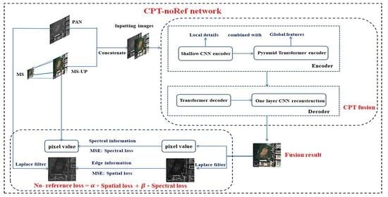
In the proposed CNN+ Pyramid Transformer network (CPT network), CNN+ Pyramid Transformer encoders are used to extract and fuse the image features. The Transformer decoder is used to enhance and obtain the final fusion features and the reconstruction is used to get the final fusion image as shown in Figure 1. Then, we designed a no-reference loss and used it to train the above CPT network to get the final CPT-noRef network. The framework of the CPT-noRef network will be introduced in detail in the following four parts.
2.2.1. CNN+ Transformer
In this paper, each band of the MS image was up-sampled to the size of the PAN image through the bilinear method to get the MS-UP image, and then they were concatenated to obtain the training data with N + 1 bands, as shown in Figure 2.
In order to solve the Transformer network needing a large amount of training set data, as well as the lack of local information supplement characteristics, we modified the input N + 1 bands of the PAN and MS images of the traditional Transformer network to the shallow image features extracted from the CNN. The architecture of the basic CNN used to extract shallow features is shown in Figure 3, and its parameters are shown in Table 2, where c1 means the band number N + 1 of the input image, c4 is the channel number 32 of the output shallow feature map, and c2 and c3 are the number of filters.(I = 1, 2, 3) means the filter kernel size and the rectified linear unit (ReLU) is used as the activation function.
2.2.2. Pyramid Structure in the Transformer
Before applying the Transformer network to the remote sensing image, the image needs to be segmented into a series of patches to obtain the serialized data which is similar to the words in a sentence. Assuming that the size of the input image is, the size of each patch is, and the image is decomposed into vectors, where and. We then computed the self-attention between these vectors. However, through this operation, we can only obtain the relationship between the patches, and the structural information in each patch is lost. So the patch size we set was always small to avoid the loss of the internal details in each patch. However, this also means the deep semantic information cannot be extracted and the global feature is inadequate. To solve this problem, we considered adding the pyramid structure into the encoder part of the Transformer to establish the contact between different feature levels by constantly changing the corresponding receptive field of each patch.
The process of the pyramid Transformer in this paper is divided into the following three parts:
- (1)
- Firstly, the shallow features () obtained from the CNN were down-sampled until the feature size is the same as the patch size. The size of is (100,100), and the patch size is (5,5), so the sizes of the sub-samples (i = 0, 1, 2, 3) were set as (100,100), (50,50), (25,25), and (5,5), respectively.
- (2)
- After each down-sampling of , was inputted into the network, respectively, to extract the corresponding features (i = 0, 1, 2, 3).
- (3)
- Finally,was up-sampled to restore the original size. All the features (i = 0, 1, 2, 3) were concatenated to obtain the feature which is the result of the pyramid Transformer encoder, where is the number of down-sampling operations and means concatenating the features on the channel dimension.
The whole pyramid structure is shown in Figure 4. The pyramid structure expands the patch receptive field by down-sampling the input feature map to extract the large-scale semantic features. While the image down-sampling will cause the loss of detail information, the patches with the small receptive fields can supply the edge contour, color distribution, and other details of the image which makes the global features extracted by the pyramid Transformer more comprehensive than the Transformer [11]. Moreover, the pyramid Transformer can reduce the sensitivity to the input feature scales by learning multi-scale feature information, which can enhance the robustness of the network to some extent.
2.2.3. Transformer for Fusion
The proposed CPT fusion method firstly extracts the shallow features of the input images through the basic CNN, and then these shallow feature maps are inputted into the Transformer network to combine the global features to ensure the sufficiency of feature extraction, which is described in Section 2.2.1. In this paper, the pyramid structure was added into the Transformer encoder in order to get the multi-scale features to enhance the robustness and improve the fusion result of the network, which has been described in detail in Section 2.2.2. In addition, the Transformer network we used for fusion consists of three parts: (1) Converting to the serialized data, (2) encoder, and (3) decoder.
- (1)
- Converting shallow features to the serialized data.
Firstly, the feature map is converted into a series of patch tokens. This process is consistent with that of ViT [18]. The difference is that we removed the learnable classification embedding in ViT because we do not need to classify the input. The size of the feature map input in this paper is , where represents the batch size of the training, represents the number of the inputting feature channels, and and are the height and width of the feature map, respectively. We set the patch size asslide the patch and reshaped the map as which is simplified as . Then, through a full connection layer in Embedding, the vectors were mapped to , , where represents the number of feature channels. The process of shallow features converting to patches is shown in Figure 5.
- (2)
- Transformer Encoder
The transformer encoder is mainly composed of the layer normalization (LN), the multi-head self-attention layer (MSA), and the multi-layer perception (MLP). These three parts are connected by the residual network structure [8], as shown in Equation (2), where is the inputting vectors converting from the feature map, and is the output of the Transformer encoder and the input of the decoder part. LN ensures the stability of network training. MSA computes self-attention in multi-heads in parallel that enables the network to capture and consider the relationship globally. MLP enhances the features by adding the channel dimension linearly, which is similar to using 1 × 1 kernel size convolution to adjust the dimension in CNN. The structure of MSA is shown in Figure 6.
In Figure 6, Q, K, V represent Query, Key, and Value, respectively, and their weight matrices are. When inputting to MSA, Q, K, V are represented by the linear transformation in Equation (3).
The matching degree between Q and K is calculated through the dot product in Attention as shown in Equation (4), where means the dimension of Q, K. Furthermore, softmax gives attention values from 0 to 1 which differentiates the levels of importance to V according to the results of the dot product of Q and K.
Each head produces an output attention vectoras shown in Equation (5). These attention vectors need to be combined to a single vector through concatenating in Equation (6), where means the number of the head.
The process of the Transformer encoder is shown in Figure 7. In addition, the position sequence relationship between patches in the Transformer is learned by embedding the position vector (the Pos Vector in Figure 7), whose size is the same as that of the feature vector, which is obtained through the process in Figure 5. Therefore, the feature vector and the position vector are combined before inputting into the encoder part of the Transformer.
- (3)
- The decoder process is similar to the process of the encoder though we added a layer containing LN and MSA in order to enhance the fusion features in Equation (7), where is the output of the encoder in Equation (2) and is the result of the decoder.
After getting the fusion features, we reshaped to , where means the dimension of the final feature channels, and then reconstructed it to the fusion result } ( means the dimension of the fusion result channels) through 1 × 1 kernel size convolution.
2.2.4. No-Reference Loss
In the course of fusion network training, the selection of loss function is also very important. The classical fusion network chooses the mean square error (MSE) as the loss function [26,27]. It can give sufficient attention to the samples with large deviation by giving them a larger weight which can quickly reduce the difference between the fusion image and the target image and make the network training more efficient.
However, at present, most ideas of deep learning image fusion still remain in the direction of creating simulated data sets. In the fusion model with simulated data, the original MS image is taken as the reference fused image, and the PAN and MS images are degraded as the input images according to the Wald protocol. This model has certain disadvantages:
- (1)
- First of all, in the process of making the training set, the PAN image needs to be down-sampled, which will lose important spatial information.
- (2)
- In the process of network training, the MS image is used as the reference image for training, so the network model cannot learn the real spatial information and the real fusion relationship.
- (3)
- In the model testing stage, real remote sensing images are used for testing which means the original PAN and MS images are tested on the network model trained by the degraded PAN and MS images. Due to the scale difference between the training data and the test data, the test result is not satisfactory.
Subsequently, Xiong has proposed the no-reference loss function through the combination of the no-reference spatial and spectral evaluation indexes based on the real PAN and MS training data, which is state-of-the-art in deep learning pan-sharpening [28,29]. Based on the idea of training the fusion network on the real data, in this paper, we propose the new no-reference loss function from another perspective based on the essence of fusion theory, making the network learn the spatial information from the inputting PAN image and the spectral information from the inputting MS image.
In terms of spatial details, it emphasizes the relationship between each pixel and its adjacent pixels in each image and seeks the transformation of attributes and directions between pixels, which is the high-frequency information of images that is spatial edge detail information. In this paper, we selected the Laplace filter for extracting the spatial details of the fusion image and the PAN image, respectively, and then the spatial information of the two images was studied by MSE. We used function to represent the two-dimensional image and to represent the gray mutation region of .
The mutation containing two diagonal angles can be calculated as [30]:
According to Equation (9), the Laplace filtering used in this paper is as follows:
After filtering, the fusion image, PAN, and MS-UP are shown in Figure 8.
The pixel digital number value of each remote sensing band image was determined by the intensity of electromagnetic radiation detected by sensors and can represent the spectral characteristics of each band image. Therefore, in terms of the spectral loss, the pixel value of the fused image and that of the MS image are directly studied by MSE, making the pixel value of the fused image as close as possible to that of the MS image.
The total loss includes spatial loss and spectral loss as shown in Equation (11):
Herein represents the weight of the spatial loss and represents the weight of the spectral loss. The sum of and equals 1.
If is set to 1, each band of the fusion result of the network will be infinitely close to the PAN image. Oppositely, if is set to 0, the output result will be close to the MS-UP image. Therefore, we set up a comparative experiment to determine the optimal values of and. The initial is set to 0.1 and is set to 0.9, respectively. They were gradually adjusted with a step of 0.1 to achieve the optimal balance between spectral and spatial information.
Figure 9 shows the quality evaluation curves of fusion images with different weights. Figure 10 shows the fusion images with different weights. We used evaluation indexes , and quality with no reference (QNR) to evaluate the fusion results with different weight values. They are defined as Equations (12)–(14):
Herein is the inputting PAN image, is the degraded PAN image whose size is the same as that of the MS image, is the fusion result, and L is the band number of inputting MS images. , are typically set to 1 and are the tradeoff coefficients, usually [31]. is the universal image quality indices defined as Equation (15), where is the covariance of x and y, are the average of x and y, and are the variance of x and y, respectively. From Equations (12)–(15), it can be concluded that measures the distance of the band correlation between fusion result and MS image. Similarly, measures the spatial consistency between the fusion result and PAN image. Therefore, the closer and are to 0, the better the evaluation index is. QNR represents the global quality of the fusion image, and the maximum theoretical value of it is 1.
As can be seen from Figure 9, whenis set to 0.2, the global quality index QNR of the fusion image is the best. Correspondingly, from Figure 10, we can see that it has a superior spectral-spatial balance ability compared with other results. Therefore, the weights of the spectral and spatial loss are set to 0.8 and 0.2, respectively, in our no-reference loss function in this paper.
3. Results
3.1. Experimental Setting
Our network model training was performed with the Pytorch framework in Linux systems and accelerated on the NVDIA GeForce RTX 3090 GPU.
The parameters settings of the experiment are shown in Table 3 and Table 4, where Table 3 is the basic parameter setting and Table 4 is the hyper-parameter setting. The number ratio of the training set to the test set was four. The network inputs included the PAN and the corresponding up-sampled MS images. The number of the training images was 102,400 pairs and that of the test images was 25,600 pairs.
For the learning rate (), if a large is used (0.1, 0.03…), the model will be unstable in the initial training stage and the accuracy of the network is seriously affected, increasing the difficulty of convergence. If a small is used (, …), the training efficiency of the network will be seriously decreased. Therefore, in our CPT-noRef, the initial learning rate () was set to according to experience. With the deepening of network training, the value of the loss gets smaller so the fixed will cause the network to fall into the local minimum value and stop learning. To avoid this problem, the step learning rate (StepLR) strategy was used to update the as shown in Equation (16), where (set as 0.3) means the adjusting multiples of , and is updated every (set as 40) epoch.
In deep learning models, the batch size is usually set to 8, 16, 32, 64,… etc.; the Transformer requires a large amount of data. The large batch size will cause the phenomenon of over-memory during training and the small batch size will increase the number of iterations in each training epoch, which will lead to a longer training time. After multiple adjustments and experimentation, the batch size was set to 16.
For the number of hidden nodes in MLP, if the number is too small, the network cannot obtain the necessary learning ability and information processing ability. On the contrary, the complexity of the network structure will be greatly increased. Therefore, in this paper, we set the number of hidden nodes to 2F + 1, where F means the number of the inputting features of MLP, according to the Kolmogorov theorem [20].
Moreover, in the structure of MSA, the number of heads needs to be determined. In our experiments, the size of the inputting training image was } and the size of 5. Therefore, we could convert the inputting image into 400 patch vectors with the size of, where means the band number of the inputting training image. When the number of heads is large, the network parallelism can be enhanced, but the network parameters will also increase. When the number is small, MSA is similar to the self-attention model, the network operation efficiency is low, and the phenomenon of over-fitting will occur. Therefore, we divided these 400 vectors into four heads for feature extraction. The optimizer for training was the Adam weight decay optimizer (AdamW) [32].
3.2. Experimental Results and Analysis
In the experiment, we compared our CPT-noRef with other seven typical deep learning fusion methods including PNN [8], improved-SRCNN [25], DRPNN [9], ResNet [33], PanNet [34], TF-ResNet [35], and GAN [36]. We evaluated the fusion effect from both the subjective vision and the objective indexes. The objective indexes we used mainly divided into three aspects: The spectral evaluation indexes—correlation coefficient (CC), spectral angle mapper (SAM), , and erreur relative global adimensionnelle de synthèse (ERGAS); the spatial evaluation indexes—structural similarity index (SSIM), ; and the comprehensive evaluation index QNR [37,38]. We also designed experiments to verify the advantages of our designed loss function with the real input data and not the simulated data again. Finally, we performed the generalization experiment to test the robustness of these fusion networks. We evaluated the fusion results in the following four parts.
3.2.1. No-Reference Loss Comparison Results
In order to verify the feasibility and effectiveness of our no-reference loss function, we selected four fusion methods including PNN, TF-ResNet, PanNet, and CPT to design a comparative experiment. In the experiment, we trained these four methods by using the with-reference loss function on the simulated data, and by using our designed loss function on the real data in order to evaluate our no-reference loss function fairly and comprehensively. The test image size of GF-1 and WV-2 is {400 × 400}. In this experiment, , and QNR are used as the evaluation indexes.
For the GF-1 data, the comparison results are shown in Figure 11 and the objective assessment is in Table 5. In Table 5 the no-reference loss network names are suffixed with noRef, and for all tables below, the bold result indicates the best result.
From a visual point of view, the spatial detail of the fusion results using our no-reference loss is significantly improved and the improvement effect of TF-ResNet and PanNet is the most outstanding, as can be seen on the roof of the buildings especially the blue one in the lower middle part of the image. Moreover, there is nearly no spectral distortion in these four methods using our loss function where the suppression effect of the spectral distortion in PNN is most obvious. Furthermore, the CPT trained with simulated data has rich spatial information but light spectral distortion.
From the objective evaluation indexes, all indexes are enhanced drastically by using our no-reference loss compared with the results using simulated data. The spectral distortion of PNN by using simulated data is serious with a large value of , but the value decreases considerably by using our loss function. The value of PanNet also decreases sharply, which means the spatial details of PanNet get much more abundant by using our no-reference loss. The proposed CPT-noRef has the best evaluation indexes wherever in spatial and spectral quality.
For the WV-2 data, the loss function comparison results are shown in Figure 12 and the quality evaluation is given in Table 6. In Table 6 the no-reference loss network names are suffixed with noRef.
In addition, we extracted five kinds of ground objects from the PNN fusion image to observe the fusion effect of PNN in detail which is shown in Figure 13. The first line is the spatial details of the fusion image trained by PNN with-reference loss and simulated data; the second line is that of the fusion image trained by our designed no-reference loss function and real data.
In Figure 13 for WV-2, the spatial details of the fusion results trained by our no-reference loss improve markedly, which can be compared directly with the fusion results trained by using the simulated data. We can see the moving cars, the pedestrian crossing, and the outline of the roof are clear in the fusion image trained by our designed loss function. Additionally, in Figure 12, the spectral distortion of the method trained by using the simulated data is serious except for CPT and PanNet. However, the fusion methods trained by our loss function can maintain the spectral quality well, except for PNN with an overall dark color.
In Table 6 for WV-2, all indexes of the method trained by our loss function are much better than that of the method trained by simulated data which is the same as the GF-1 training results. Among methods trained by using the simulated data, the evaluation index of CPT is the best, but the value can decrease further after using our designed loss. In all evaluation indicators, CPT-noRef (our method) surpasses other methods.
3.2.2. GF-1 Remote Sensing Data Results
In order to better compare the fusion effect of different methods for GF-1 remote sensing images, urban scenes (as shown in Figure 14) and rural scenes (as shown in Figure 15 and Figure 16) were selected for testing. The quantitative evaluation results of these two scene types are provided in Table 7 and Table 8, respectively.
For the urban scenes of the GF-1 remote sensing image test experimental results, the size of each image is }.
From the visual point of view, it can be seen from the red box in Figure 14, the spatial details of our method are far clearer than other methods, especially in the built-up areas and on the roofs of buildings; the spatial information of PNN, TF-ResNet, and ResNet are also good. For the spectral quality, our CPT-noRef method, ResNet, and PanNet are basically consistent with the MS-UP image. PNN, DRPNN, and GAN have some spectral distortion.
Considering the objective evaluation indexes, all evaluation indexes of our method are the best, and the values of and significantly surpass that of other methods. ResNet, PanNet, and TF-ResNet also have good spectral retention ability, next to our CPT-noRef. On the contrary, the spectral distortion of PNN, DRPNN, and GAN is serious, which is the same as the subjective evaluation, and GAN has the worst spectral fidelity. Moreover, the spatial details of PNN and TF-ResNet are abundant with good value of , but GAN and DRPNN methods have insufficient spatial information. The evaluation index of the improved-SRCNN is generally average.
In order to show the fusion effect of different band combinations and different landscapes, we cropped two rural fields as shown in Figure 15 and Figure 16 with false and true color compositions, respectively. The size of each result in Figure 15 is , and that of each result in Figure 16 is .
From the perspective of subjective vision, the proposed CPT-noRef has the richest spatial information; the texture of the river and arable land can clearly be seen in Figure 16j. The spatial information of PNN, TF-ResNet, and GAN enhances sizably, as shown in Figure 15, but the spatial information of improved-SRCNN and DRPNN is fuzzy. The spectral quality of the CPT-noRef, PanNet, and ResNet images are similar to that of the MS-UP image. In contrast, the spectral characteristics of PNN and GAN are not satisfactory.
According to the objective evaluation indexes in Table 8, the evaluation indexes of our method are still the best in the rural region. The spatial information of PNN and TF-ResNet is rich with a good value of and SSIM. Compared to the fusion result for the urban scenes, the spatial quality of GAN greatly improves. Oppositely, the spatial details of PanNet, improved-SRCNN, and DRPNN are insufficient. As for the spectral information, in addition to the CPT-noRef, the spectral retention ability of PanNet, ResNet, and TF-ResNet is excellent. PNN and GAN have the poor learning ability of spectral characteristics. The spectral retention of DRPNN and improved-SRCNN is moderate.
3.2.3. WV-2 Remote Sensing Data Results
In order to better compare the fusion effect of different methods, we cropped the vegetation (the size is) and highway region (the size is) in the urban scenes of the test image for concrete display as shown in Figure 17 and Figure 18, respectively. The quantitative evaluation result of the test image is in Table 9.
From the red box of the vegetation region, we know that the spatial information of CPT-noRef, TF-ResNet, and GAN is more abundant than others, which can be seen from the clear leaf textures. The spectral quality of CPT-noRef, PanNet, and improved-SRCNN is similar to that of the MS-UP image. In the vegetation region, the road color of PNN, DRPNN, ResNet, and GAN is lighter than that of MS-UP and the spectral distortion of GAN is serious. The color of the green leaves in the TF-ResNet image is darker than others. The visual effect of the highway image is similar to that of the vegetation region, and the magnified parked vehicles in the red box in each image can highlight the spatial enhancement advantages of CPT-noRef, TF-ResNet, and GAN, and the disadvantages of PanNet and improved-SRCNN.
From the objective evaluation indexes, the , values of CPT-noRef and GAN are outstanding followed by TF-ResNet. On the contrary, the spatial effect of PanNet and improved-SRCNN is not satisfactory with a large value of and little value of . Moreover, from the value of and the spectral retention ability of CPT-noRef surpasses other methods. PanNet and improved-SRCNN also have good spectral maintaining ability. The spectral distortion of GAN, DRPNN, TF-ResNet, and PNN is much more serious with the bad value of spectral evaluation indexes.
3.2.4. Generalization Experiment Results
In order to verify the robustness and the stability of our CPT-noRef method, we use the network model trained by GF-1 to conduct the cross-sensor generalization experiments on Pleiades and WV-2 data (the size is {400 × 400}) directly and compare the visual effect of our method with that of other seven methods. The Pleiades image generalization results based on the model trained by the GF-1 data are shown in Figure 19.
The WV-2 image generalization results based on the model trained by the GF-1 data are shown in Figure 20.
From Figure 19 and Figure 20, we can see that the spectral distortion of PNN and ResNet is serious, which will cause misjudgment of the ground objects. PNN loses much spatial information simultaneously. We can hardly see the details of the ground objects in PNN. The fusion color of DRPNN and GAN is darker than that of the MS-UP image, and that of TF-ResNet is brighter. PanNet, improved-SRCNN, and CPT-noRef have excellent spectral preservation ability, but the spatial information of PanNet and improved-SRCNN is fuzzy. We cannot see the image details like the cars in the parking lot in Figure 19h,i, and the roof of the buildings in Figure 20h,i. Our method is overwhelmingly superior in the two generalization experiments, which confirms that our method has strong generalization ability. The reason is because the CPT-noRef method can extract comprehensive image features by combining the short-distance local features with the long-distance global features. Moreover, our loss function which extracts the edge information of PAN and the pixel value of MS-UP can make the CPT-noRef network learn the real fusion relationship between input and output.
3.2.5. The Time Performance of the Algorithm
Taking the GF-1 image training time as an example, the time performance of different methods with two loss functions are shown in Table 10 and Table 11, respectively. The epoch number in Table 10 and Table 11 is the number of training times when each network reaches its optimal convergence.
The input of the network with no-reference loss is the real PAN and up-sampled MS image and the input of the network with reference loss is the degraded simulated PAN and MS image. The spatial resolution of the real image is four times that of the degraded image. Therefore, the amount of the input training data in the no-reference network is 16 times that of the reference network. For intuitive comparison, we added the equivalent time in Table 11 making sure the input data amount of the two networks are equal.
According to the training time, CPT has high training efficiency due to the high degree of parallelization of the Transformer, whose training time is between the three-layer convolutional PNN network and the four-layer convolutional improved-SRCNN network. Moreover, the loss function we designed in this paper can also improve the operating efficiency of the network to some extent.
4. Discussion
According to the ablation experiment results in Section 3.2.1, it is found that the designed no-reference loss can significantly help the fusion network (whether simple or complex) improve the spatial information and maintain the spectral quality. Meanwhile, the proposed no-reference loss is based on real data, which can solve the problem of scale difference between the test image and training image and improve the fusion effect of the testing and real data.
Through the fusion experiments of different sensor (GF-1, WV-2) images in Section 3.2.2 and Section 3.2.3, it can be seen that except for the CPT-noRef, the other seven fusion methods show different fusion effects on different sensor images. Through the qualitative and quantitative evaluation indicators, we can conclude that for PNN in GF-1 image fusion, the improvement of spatial information is good, but its spectral distortion is serious. However, in WV-2 image fusion, PNN learns the poor spatial information and the spectral quality of it is still unsatisfactory. For GAN, in the urban scenes of the GF-1 image, the spatial and spectral information is the worst among these methods, but the spatial information enhances considerably in the rural scenes. Moreover, in the WV-2 image fusion, the spatial information of GAN is rich, and its spatial evaluation indexes rank second among these methods. For TF-ResNet in the fusion of GF-1, whether for the urban or rural scenes, the overall fusion effect is excellent, but it has bad spectral fidelity in WV-2 fusion. The spectral quality of improved-SRCNN enhances markedly in WV-2 fusion, but that of ResNet decreases slightly compared to the GF-1 fusion results. In the two sensor fusion experiments, PanNet has the superior spectral retention capability, but its spatial effect is always fuzzy which means the spectral quality is maintained but it neglects to enhance the spatial information. The spatial information of DRPNN is inadequate in GF-1 fusion and the effect of it in WV-2 fusion is not outstanding both in the spectral and spatial information. The proposed CPT-noRef method performs best in both spectral and spatial information which can lead to the conclusion that the adequacy of multi-scale feature extraction can enhance the stability of the network and its no-reference loss can help it learn the real fusion relationship between the input image and the fusion image. Its excellent generalization ability can be clearly seen when fusing the cross-sensor and cross-scale images in the experiments in Section 3.2.4.
From the time performance test in Section 3.2.5, we know that the training time of PNN and improved-SRCNN is relatively fast because their structures are shallow. PanNet improves the operating efficiency by only learning spatial information in the high-frequency area of the image. The training time of DRPNN and ResNet increases to a certain extent because they have residual structures which make the networks more complex than others. GAN takes a long time to train generators and discriminators separately. TF-ResNet is divided into two branches to extract the information of PAN and MS images. The two-stream residual networks have a large number of parameters, and the extracted information of the image is rich, so the workload of fusion is large. The training efficiency of the proposed CPT network is high because of a high degree of parallelization of the Transformer in it. With the advantage of the Transformer’s outstanding global feature extraction ability, the global contextual information is directly combined with the detailed local information extracted from the shallow CNN, which can avoid adding the complexity of the CNN. Moreover, the loss function we designed can slightly increase the network training speed, which can be seen in Table 11.
5. Conclusions
The proposed CPT-noRef can solve the huge amount of data required by the Transformer network, improve the operation efficiency of the network, and control the loss of spatial and spectral aspects simultaneously. The global contextual information from the Transformer was combined with the local feature information from shallow CNN to ensure the adequacy of the feature extraction. Since the pyramid structure was added to the Transformer encoder, the robustness of CPT-noRef was enhanced by extracting multi-scale features. Moreover, our designed no-reference loss function made the learning target change to learn the spatial information from the inputting PAN image and the spectral information from the inputting MS image. The reference labels were changed to inputting PAN and MS themselves, not the simulated high-resolution data, which broke through the fusion framework of the current fusion network and improved the fusion effect considerably. In this paper, different GF-1, Pleiades, and WV-2 remote sensing satellite data with different land covers were used to verify the effectiveness of our CPT-noRef method through fusion and generalization experiments. Furthermore, we also designed an experiment to test the feasibility and validity of our no-reference loss function by applying it to four fusion networks. The results demonstrated that the proposed CPT-noRef method achieves state-of-art performance in terms of both visual perception and objective assessment. Our loss function, which is consistent with the theory of fusion, only used the original PAN and MS data themselves as the reference labels, making the network monitor both the spatial and spectral loss and surpassing the fusion result trained by the simulated degraded data.
The proposed CPT-noRef directly stacked the PAN and up-sampled MS together as the inputting images for further processing. The features of PAN and MS were treated equally, which may decrease the reconstruction quality to some extent. In addition, all the features extracted from the pyramid Transformer encoder were equally concatenated on the channel dimension which ignored the importance of certain features. In following work, we will consider using a two-stream fusion framework to fully extract the features of the PAN and MS images, respectively. Moreover, we will try to use a channel attention mechanism module to replace the commonly used concatenation operation, considering the relationship between different channels, thereby improving the quality of feature fusion.
Author Contributions
Q.G. proposed the research concept, analyzed the feasibility of the method, provided the experimental data, participated in analyzing the results, and reviewed and revised the manuscript. S.L. designed the framework and the flow of this research, processed the experimental data, designed the network, conducted the experiments, analyzed the result, and wrote the manuscript. A.L. reviewed the manuscript and revised the figures. All authors have read and agreed to the published version of the manuscript.
Funding
This research was funded in part by the National Natural Science Foundation of China, grant number 61771470 and in part by the Strategic Priority Research Program of the Chinese Academy of Sciences, grant number XDA19010401 and XDA19060103.
Institutional Review Board Statement
Not applicable.
Informed Consent Statement
Not applicable.
Data Availability Statement
We are very grateful for the GF-1 data provided by the China Centre for Resources Satellite Data and Application. Meanwhile, we used the WV2 experimental data from DigitalGlobe’s high-resolution commercial satellite and the Pleiades experimental data from the Astrium GEO-Information Services satellite.
Acknowledgments
We are very grateful to the reviewers who significantly contributed to the improvement of this paper.
Conflicts of Interest
The authors declare no conflict of interest.
Abbreviations
All the acronyms used in this paper are listed as follows.
| Acronyms | The Full Name |
| CNN | convolutional neural network |
| PAN | panchromatic |
| MS | multi-spectral |
| Fast RCNN | fast region-CNN |
| RFCN | region-based fully convolutional networks |
| CPT | CNN+ pyramid Transformer |
| CPT-noRef | CPT with no-reference loss |
| WV-2 | WorldView-2 |
| GF-1 | Gaofen-1 |
| PNN | pan-sharpening method based on CNN |
| ReLU | rectified linear unit |
| LN | layer normalization |
| MSA | multi-head self-attention layer |
| MLP | multi-layer perception |
| AdamW | Adam weight decay optimizer |
| StepLR | step learning rate |
| P | inputting PAN image |
| Pdg | degraded PAN image |
| fused | fusion result |
| UQI | universal image quality indices |
| Lr | learning rate |
| initiallr | initial learning rate |
| p | patch size |
| ViT | vision Transformer |
| MSE | mean square error |
| CC | correlation coefficient |
| SSIM | structural similarity index |
| ERGAS | erreur relative global adimensionnelle de synthèse |
| SAM | spectral angle mapper |
| QNR | quality with no reference |
References
- Witharana, C.; Bhuiyan, A.E.; Liljedahl, A.K.; Kanevskiy, M.; Epstein, H.E.; Jones, B.M.; Daanen, R.; Griffin, C.G.; Kent, K.; Jones, M.K.W. Understanding the synergies of deep learning and data fusion of multispectral and panchromatic high resolution commercial satellite imagery for automated ice-wedge polygon detection. J. Photogramm. Remote Sens. 2020, 170, 174–191. [Google Scholar] [CrossRef]
- Siok, K.; Ewiak, I.; Jenerowicz, A. Multi-Sensor Fusion: A Simulation Approach to Pansharpening Aerial and Satellite Images. Sensors 2020, 20, 7100. [Google Scholar] [CrossRef] [PubMed]
- Zhang, W.; Liljedahl, A.K.; Kanevskiy, M.; Epstein, H.E.; Jones, B.M.; Jorgenson, M.T.; Kent, K. Transferability of the Deep Learning Mask R-CNN Model for Automated Mapping of Ice-Wedge Polygons in High-Resolution Satellite and UAV Images. Remote Sens. 2020, 12, 1085. [Google Scholar] [CrossRef] [Green Version]
- Gkioxari, G.; Girshick, R.; Malik, J. Actions and Attributes from Wholes and Parts. In Proceedings of the 2015 IEEE International Conference on Computer Vision (ICCV), Santiago, Chile, 7–13 December 2015; pp. 2470–2478. [Google Scholar] [CrossRef] [Green Version]
- Ren, S.; He, K.; Girshick, R.; Sun, J. Faster R-CNN: Towards Real-Time Object Detection with Region Proposal Networks. IEEE Trans. Pattern Anal. Mach. Intell. 2017, 39, 1137–1149. [Google Scholar] [CrossRef] [Green Version]
- Lin, T.-Y.; Goyal, P.; Girshick, R.; He, K.; Dollár, P. Focal Loss for Dense Object Detection. IEEE Trans. Pattern Anal. Mach. Intell. 2020, 42, 318–327. [Google Scholar] [CrossRef] [Green Version]
- Dai, J.F.; Li, Y.; He, K.M.; Sun, J. R-FCN: Object Detection via Region-based Fully Convolutional Networks. In Proceedings of the Advances in Neural Information Processing Systems, Barcelona, Spain, 5–10 December 2016; pp. 379–387. [Google Scholar]
- Masi, G.; Cozzolino, D.; Verdoliva, L.; Scarpa, G. Pansharpening by Convolutional Neural Networks. Remote Sens. 2016, 8, 594. [Google Scholar] [CrossRef] [Green Version]
- Wei, Y.; Yuan, Q.; Shen, H.; Zhang, L. Boosting the Accuracy of Multispectral Image Pansharpening by Learning a Deep Residual Network. IEEE Geosci. Remote Sens. Lett. 2017, 14, 1795–1799. [Google Scholar] [CrossRef] [Green Version]
- Rao, Y.; He, L.; Zhu, J. A residual convolutional neural network for pan-shaprening. In Proceedings of the 2017 International Workshop on Remote Sensing with Intelligent Processing (RSIP), Shanghai, China, 18–21 May 2017; pp. 1–4. [Google Scholar] [CrossRef]
- Wang, F.; Guo, Q.; Ge, X. Pan-sharpening by deep recursive residual network. J. Remote Sens. 2021, 25, 1244–1256. [Google Scholar] [CrossRef]
- Chen, M.; Guo, Q.; Liu, M. Pan-sharpening by residual network with dense convolution for remote sensing images. J. Remote Sens. 2021, 25, 1270–1283. [Google Scholar] [CrossRef]
- Wu, Y.; Huang, M.; Li, Y.; Feng, S.; Wu, D. A Distributed Fusion Framework of Multispectral and Panchromatic Images Based on Residual Network. Remote Sens. 2021, 13, 2556. [Google Scholar] [CrossRef]
- Vitale, S.; Scarpa, G. A Detail-Preserving Cross-Scale Learning Strategy for CNN-Based Pansharpening. Remote Sens. 2020, 12, 348. [Google Scholar] [CrossRef] [Green Version]
- Wang, W.; Zhou, Z.; Liu, H.; Xie, G. MSDRN: Pansharpening of Multispectral Images via Multi-Scale Deep Residual Network. Remote Sens. 2021, 13, 1200. [Google Scholar] [CrossRef]
- Naushad, R.; Kaur, T.; Ghaderpour, E. Deep Transfer Learning for Land Use and Land Cover Classification: A Comparative Study. Sensors 2021, 21, 8083. [Google Scholar] [CrossRef] [PubMed]
- Xu, H.; Le, Z.; Huang, J.; Ma, J. A Cross-Direction and Progressive Network for Pan-Sharpening. Remote Sens. 2021, 13, 3045. [Google Scholar] [CrossRef]
- Tuli, S.; Dasgupta, I.; Grant, E.; Griffiths, T.L. Are Convolutional Neural Networks or Transformers more like human vision? arXiv 2021, arXiv:2105.07197. [Google Scholar]
- Vaswani, A.; Shazeer, N.; Parmar, N.; Uszkoreit, J.; Jones, L.; Gomez, A.N.; Kaiser, L.; Polosukhin, I. Attention is all you need. In Proceedings of the 31st Conference on Neural Information Processing Systems (NIPS 2017), Long Beach, CA, USA, 4–9 December 2017; pp. 5998–6008. [Google Scholar]
- Dosovitskiy, A.; Beyer, L.; Kolesnikov, A.; Weissenborn, D.; Zhai, X.; Unterthiner, T.; Dehghani, M.; Minderer, M.; Heigold, G.; Gelly, S.; et al. An Image is Worth 16 × 16 Words: Transformers for Image Recognition at Scale. arXiv 2020, arXiv:2010.11929. [Google Scholar]
- Zhu, X.; Su, W.; Lu, L.; Li, B.; Wang, X.; Dai, J. Deformable DETR: Deformable Transformers for End-to-End Object Detection. arXiv 2020, arXiv:2010.04159. [Google Scholar]
- Zheng, S.; Lu, J.; Zhao, H.; Zhu, X.; Luo, Z.; Wang, Y.; Fu, Y.; Feng, J.; Xiang, T.; Torr, P.H.; et al. Rethinking Semantic Segmentation from a Sequence-to-Sequence Perspective with Transformers. arXiv 2020, arXiv:2012.15840. [Google Scholar]
- Fu, Y.; Xu, T.; Wu, X.; Kittler, J. PPT Fusion: Pyramid Patch Transformer for a Case Study in Image Fusion. arXiv 2021, arXiv:2107.13967. [Google Scholar]
- Wald, L.; Ranchin, T.; Mangolini, M. Fusion of satellite images of different spatial resolutions: Assessing the quality of resulting images. Photogramm. Eng. Remote Sens. 1997, 63, 691–699. [Google Scholar]
- Xiong, Z.; Guo, Q.; Liu, M.; Li, A. Pan-Sharpening Based on Convolutional Neural Network by Using the Loss Function With No-Reference. IEEE J. Sel. Top. Appl. Earth Obs. Remote Sens. 2021, 14, 897–906. [Google Scholar] [CrossRef]
- Li, Z.; Cheng, C. A CNN-Based Pan-Sharpening Method for Integrating Panchromatic and Multispectral Images Using Landsat 8. Remote Sens. 2019, 11, 2606. [Google Scholar] [CrossRef] [Green Version]
- Scarpa, G.; Vitale, S.; Cozzolino, D. Target-Adaptive CNN-Based Pansharpening. IEEE Trans. Geosci. Remote Sens. 2018, 56, 5443–5457. [Google Scholar] [CrossRef] [Green Version]
- Xiong, Z.; Guo, Q.; Liu, M.; Li, A. Pan-Sharpening Based on Panchromatic Image Spectral Learning Using WorldView-2. IEEE Geosci. Remote Sens. Lett. 2021, 19, 1–5. [Google Scholar] [CrossRef]
- Xiong, Z.; Guo, Q.; Liu, M.; Li, A. Pan-Sharpening Based on Panchromatic Colorization Using WorldView-2. IEEE Access 2021, 9, 115523–115534. [Google Scholar] [CrossRef]
- Podlubny, I. The Laplace transform method for linear differential equations of the fractional order. arXiv 1997, arXiv:funct-an/9710005. [Google Scholar]
- Alparone, L.; Aiazzi, B.; Baronti, S.; Garzelli, A.; Nencini, F.; Selva, M. Multispectral and Panchromatic Data Fusion Assessment Without Reference. Photogramm. Eng. Remote Sens. 2008, 74, 193–200. [Google Scholar] [CrossRef] [Green Version]
- Yao, Z.; Gholami, A.; Shen, S.; Mustafa, M.; Kurt, K.; Mahoney, M.W. ADAHESSIAN: An adaptive second order optimizer for machine learning. arXiv 2020, arXiv:2006.00719. [Google Scholar]
- Wei, Y.; Yuan, Q. Deep residual learning for remote sensed imagery pansharpening. In Proceedings of the 2017 International Workshop on Remote Sensing with Intelligent Processing (RSIP), Shanghai, China, 18–21 May 2017; pp. 1–4. [Google Scholar]
- Yang, J.; Fu, X.; Hu, Y.; Huang, Y.; Ding, X.; Paisley, J. PanNet: A Deep Network Architecture for Pan-Sharpening. In Proceedings of the 2017 IEEE International Conference on Computer Vision (ICCV), Venice, Italy, 22–29 October 2017; pp. 1753–1761. [Google Scholar] [CrossRef]
- Liu, X.; Liu, Q.; Wang, Y. Remote sensing image fusion based on two-stream fusion network. Inf. Fusion 2020, 55, 1–15. [Google Scholar] [CrossRef] [Green Version]
- Ma, J.; Yu, W.; Chen, C.; Liang, P.; Guo, X.; Jiang, J. Pan-GAN: An unsupervised pan-sharpening method for remote sensing image fusion. Inf. Fusion 2020, 62, 110–120. [Google Scholar] [CrossRef]
- Vivone, G.; Alparone, L.; Chanussot, J.; Mura, M.D.; Garzelli, A.; Licciardi, G.A.; Restaino, R.; Wald, L. A Critical Comparison Among Pansharpening Algorithms. IEEE Trans. Geosci. Remote Sens. 2014, 53, 2565–2586. [Google Scholar] [CrossRef]
- Alparone, L.; Wald, L.; Chanussot, J.; Thomas, C.; Gamba, P.; Bruce, L.M. Comparison of Pansharpening Algorithms: Outcome of the 2006 GRS-S Data-Fusion Contest. IEEE Trans. Geosci. Remote Sens. 2007, 45, 3012–3021. [Google Scholar] [CrossRef] [Green Version]
Figure 1.
The fusion framework.

Figure 2.
The preprocessing of training data.

Figure 3.
The architecture of CNN.

Figure 4.
The pyramid Transformer encoder.

Figure 5.
Converting to patches.

Figure 6.
The MSA structure.

Figure 7.
Transformer encoder structure.

Figure 8.
The spatial information of (a) fusion, (b) PAN, and (c) MS-UP image.

Figure 9.
, , and QNR indexes of the fusion results with different values of (0.1–0.9): (a) , (b) , and (c) QNR.
Figure 9.
, , and QNR indexes of the fusion results with different values of (0.1–0.9): (a) , (b) , and (c) QNR.

Figure 10.
The visual effect of fusion results with different weight values of (0.1–0.9): (a) 0.1, (b) 0.2, (c) 0.3, (d) 0.4, (e) 0.5, (f) 0.6, (g) 0.7, (h) 0.8, and (i) 0.9.
Figure 10.
The visual effect of fusion results with different weight values of (0.1–0.9): (a) 0.1, (b) 0.2, (c) 0.3, (d) 0.4, (e) 0.5, (f) 0.6, (g) 0.7, (h) 0.8, and (i) 0.9.

Figure 11.
GF-1 true color (R, G, B) fusion results trained by using different loss function: (a) PAN, (b) MS-UP, (c) PNN, (d) TF-ResNet, (e) PanNet, (f) CPT, (g) PNN-noRef, (h) TF-ResNet-noRef, (i) PanNet-noRef, and (j) CPT-noRef (proposed method).
Figure 11.
GF-1 true color (R, G, B) fusion results trained by using different loss function: (a) PAN, (b) MS-UP, (c) PNN, (d) TF-ResNet, (e) PanNet, (f) CPT, (g) PNN-noRef, (h) TF-ResNet-noRef, (i) PanNet-noRef, and (j) CPT-noRef (proposed method).

Figure 12.
WV-2 true color (R, G, B) fusion results trained by using different loss function: (a) PAN, (b) MS-UP, (c) PNN, (d) TF-ResNet, (e) PanNet, (f) CPT, (g) PNN-noRef, (h) TF-ResNet-noRef, (i) PanNet-noRef, and (j) CPT-noRef (proposed method).
Figure 12.
WV-2 true color (R, G, B) fusion results trained by using different loss function: (a) PAN, (b) MS-UP, (c) PNN, (d) TF-ResNet, (e) PanNet, (f) CPT, (g) PNN-noRef, (h) TF-ResNet-noRef, (i) PanNet-noRef, and (j) CPT-noRef (proposed method).

Figure 13.
WV-2 comparison of the details of the objects in PNN trained by different loss functions: The first line is for PNN with reference loss, the second line is for PNN with no-reference loss. (a) the crossroads; (b) the cars; (c) the roof 1; (d) the zebra crossing; and (e) the roof 2.
Figure 13.
WV-2 comparison of the details of the objects in PNN trained by different loss functions: The first line is for PNN with reference loss, the second line is for PNN with no-reference loss. (a) the crossroads; (b) the cars; (c) the roof 1; (d) the zebra crossing; and (e) the roof 2.

Figure 14.
GF-1 true color (R, G, B) fusion results for the urban scenes: (a) PAN, (b) MS-UP, (c) PNN, (d) DRPNN, (e) ResNet, (f) TF-ResNet, (g) GAN, (h) PanNet, (i) improved-SRCNN, and (j) CPT-noRef (proposed method).
Figure 14.
GF-1 true color (R, G, B) fusion results for the urban scenes: (a) PAN, (b) MS-UP, (c) PNN, (d) DRPNN, (e) ResNet, (f) TF-ResNet, (g) GAN, (h) PanNet, (i) improved-SRCNN, and (j) CPT-noRef (proposed method).


Figure 15.
GF-1 false color (NIR, R, G) fusion results for the rural scene 1: (a) PAN, (b) MS-UP, (c) PNN, (d) DRPNN, (e) ResNet, (f) TF-ResNet, (g) GAN, (h) PanNet, (i) improved-SRCNN, and (j) CPT-noRef (proposed method).
Figure 15.
GF-1 false color (NIR, R, G) fusion results for the rural scene 1: (a) PAN, (b) MS-UP, (c) PNN, (d) DRPNN, (e) ResNet, (f) TF-ResNet, (g) GAN, (h) PanNet, (i) improved-SRCNN, and (j) CPT-noRef (proposed method).

Figure 16.
GF-1 true color (R, G, B) fusion results for the rural scene 2: (a) PAN, (b) MS-UP, (c) PNN, (d) DRPNN, (e) ResNet, (f) TF-ResNet, (g) GAN, (h) PanNet, (i) improved-SRCNN, and (j) CPT-noRef (proposed method).
Figure 16.
GF-1 true color (R, G, B) fusion results for the rural scene 2: (a) PAN, (b) MS-UP, (c) PNN, (d) DRPNN, (e) ResNet, (f) TF-ResNet, (g) GAN, (h) PanNet, (i) improved-SRCNN, and (j) CPT-noRef (proposed method).

Figure 17.
WV-2 true color (R, G, B) fusion results in vegetation region: (a) PAN, (b) MS-UP, (c) PNN, (d) DRPNN, (e) ResNet, (f) TF-ResNet, (g) GAN, (h) PanNet, (i) improved-SRCNN, and (j) CPT-noRef (proposed method).
Figure 17.
WV-2 true color (R, G, B) fusion results in vegetation region: (a) PAN, (b) MS-UP, (c) PNN, (d) DRPNN, (e) ResNet, (f) TF-ResNet, (g) GAN, (h) PanNet, (i) improved-SRCNN, and (j) CPT-noRef (proposed method).

Figure 18.
WV-2 true color (R, G, B) fusion results in highway region: (a) PAN, (b) MS-UP, (c) PNN, (d) DRPNN, (e) ResNet, (f) TF-ResNet, (g) GAN, (h) PanNet, (i) improved-SRCNN, and (j) CPT-noRef (proposed method).
Figure 18.
WV-2 true color (R, G, B) fusion results in highway region: (a) PAN, (b) MS-UP, (c) PNN, (d) DRPNN, (e) ResNet, (f) TF-ResNet, (g) GAN, (h) PanNet, (i) improved-SRCNN, and (j) CPT-noRef (proposed method).

Figure 19.
The true color (R, G, B) generalized image testing on Pleiades image: (a) PAN, (b) MS-UP, (c) PNN, (d) DRPNN, (e) ResNet, (f) TF-ResNet, (g) GAN, (h) PanNet, (i) improved-SRCNN, and (j) CPT-noRef (proposed method).
Figure 19.
The true color (R, G, B) generalized image testing on Pleiades image: (a) PAN, (b) MS-UP, (c) PNN, (d) DRPNN, (e) ResNet, (f) TF-ResNet, (g) GAN, (h) PanNet, (i) improved-SRCNN, and (j) CPT-noRef (proposed method).

Figure 20.
The true color (R, G, B) generalized image testing on WV2 image: (a) PAN, (b) MS-UP, (c) PNN, (d) DRPNN, (e) ResNet, (f) TF-ResNet, (g) GAN, (h) PanNet, (i) improved-SRCNN, and (j) CPT-noRef (proposed method).
Figure 20.
The true color (R, G, B) generalized image testing on WV2 image: (a) PAN, (b) MS-UP, (c) PNN, (d) DRPNN, (e) ResNet, (f) TF-ResNet, (g) GAN, (h) PanNet, (i) improved-SRCNN, and (j) CPT-noRef (proposed method).


Table 1.
The information of remote sensing sensor data.
| Band Number | Spatial Resolution/(m) | Location | Landscape | ||
|---|---|---|---|---|---|
| MS | PAN | ||||
| GF-1 | 1PAN + 4MS | 8 | 2 | Beijing | Rural + Urban |
| Pleiades | 1PAN + 4MS | 2 | 0.5 | Shandong | Urban |
| WV-2 | 1PAN + 8MS | 2 | 0.5 | Washington, DC | Urban |
Table 2.
The parameters of CNN structure.
| 1st ConV | 2st ConV | 3st ConV | |||||||
|---|---|---|---|---|---|---|---|---|---|
| c1 | f1(x) | c2 | f2(x) | c3 | f2(x) | c4 | |||
| N + 1 | 9 × 9 | ReLU | 16 | 5 × 5 | ReLU | 32 | 5 × 5 | ReLU | 32 |
Table 3.
The basic training parameters settings of the experiment.
| The Basic Training Parameters | |
|---|---|
| Number of training sets (PAN/MS-UP) | 102,400 |
| Number of test sets (PAN/MS-UP) | 25,600 |
| The size of the training image data | [100 × 100] |
| The size of patch size | 5 |
Table 4.
The hyper-parameters settings of the experiment.
| The Hyper-Parameters Settings | |
|---|---|
| The batch size | 16 |
| Number of the hidden nodes in MLP | 2 × F + 1 (F means the number of input features) |
| Number of the heads in MSA | 4 |
Table 5.
GF-1 objective evaluation indexes of the model trained by different loss functions.
| PNN | 0.8006 | 0.0421 | 0.1642 |
| TF-ResNet | 0.8891 | 0.0727 | 0.0412 |
| PanNet | 0.8530 | 0.1284 | 0.0213 |
| CPT | 0.9201 | 0.0560 | 0.0253 |
| PNN-noRef | 0.9437 | 0.0330 | 0.0241 |
| TF-ResNet-noRef | 0.9531 | 0.0273 | 0.0201 |
| PanNet-noRef | 0.9548 | 0.0314 | 0.0142 |
| CPT-noRef | 0.9675 | 0.0224 | 0.0103 |
Table 6.
WV-2 objective evaluation indexes of the model trained by different loss functions.
| PNN | 0.7027 | 0.0410 | 0.2673 |
| TF-ResNet | 0.7312 | 0.0237 | 0.2510 |
| PanNet | 0.8380 | 0.0702 | 0.0987 |
| CPT | 0.9015 | 0.0245 | 0.0759 |
| PNN-noRef | 0.8905 | 0.0101 | 0.1004 |
| TF-ResNet-noRef | 0.9086 | 0.0089 | 0.0832 |
| PanNet-noRef | 0.9073 | 0.0214 | 0.0728 |
| CPT-noRef | 0.9283 | 0.0066 | 0.0655 |
Table 7.
GF-1 objective evaluation indexes for the urban scenes.
| PNN | 0.9648 | 1.0163 | 0.8006 | 0.0421 | 0.1642 | 0.9693 | 1.2815 |
| DRPNN | 0.9720 | 0.9517 | 0.7770 | 0.1310 | 0.1059 | 0.9479 | 1.2076 |
| ResNet | 0.9835 | 0.8389 | 0.8969 | 0.0731 | 0.0324 | 0.9587 | 1.0325 |
| TF-ResNet | 0.9814 | 0.8430 | 0.8891 | 0.0727 | 0.0412 | 0.9593 | 1.1504 |
| GAN | 0.9607 | 1.0829 | 0.6972 | 0.1433 | 0.1862 | 0.9453 | 1.2681 |
| PanNet | 0.9846 | 0.8279 | 0.8530 | 0.1284 | 0.0213 | 0.9486 | 0.9875 |
| Improved-SRCNN | 0.9785 | 0.9498 | 0.8131 | 0.1113 | 0.0851 | 0.9490 | 1.1842 |
| CPT-noRef | 0.9887 | 0.8042 | 0.9675 | 0.0224 | 0.0103 | 0.9876 | 0.8179 |
Table 8.
GF-1 objective evaluation indexes for the rural scenes.
| PNN | 0.9751 | 0.9320 | 0.8388 | 0.0392 | 0.1270 | 0.9825 | 1.2610 |
| DRPNN | 0.9810 | 0.8420 | 0.8282 | 0.1113 | 0.0681 | 0.9413 | 1.2342 |
| ResNet | 0.9852 | 0.8350 | 0.9073 | 0.0712 | 0.0232 | 0.9601 | 0.9547 |
| TF-ResNet | 0.9824 | 0.8342 | 0.9239 | 0.0521 | 0.0253 | 0.9643 | 0.9530 |
| GAN | 0.9598 | 1.1003 | 0.8002 | 0.0673 | 0.1421 | 0.9619 | 1.3230 |
| PanNet | 0.9873 | 0.8101 | 0.8955 | 0.0925 | 0.0132 | 0.9510 | 0.9421 |
| Improved-SRCNN | 0.9776 | 0.9232 | 0.8240 | 0.1210 | 0.0625 | 0.9421 | 1.0103 |
| CPT-noRef | 0.9895 | 0.7988 | 0.9763 | 0.0136 | 0.0102 | 0.9912 | 0.7213 |
Table 9.
WV-2 objective evaluation indexes.
| PNN | 0.9421 | 1.5258 | 0.7027 | 0.0410 | 0.2673 | 0.9554 | 1.6237 |
| DRPNN | 0.9473 | 1.5227 | 0.7061 | 0.0432 | 0.2620 | 0.9549 | 1.5468 |
| ResNet | 0.9582 | 1.1846 | 0.8088 | 0.0322 | 0.1643 | 0.9643 | 1.3499 |
| TF-ResNet | 0.9495 | 1.3418 | 0.7312 | 0.0237 | 0.2510 | 0.9737 | 1.4429 |
| GAN | 0.9249 | 1.4238 | 0.7058 | 0.0181 | 0.2812 | 0.9797 | 1.7136 |
| PanNet | 0.9731 | 0.8909 | 0.8380 | 0.0702 | 0.0987 | 0.9355 | 0.9631 |
| Improved-SRCNN | 0.9625 | 0.8965 | 0.8433 | 0.0619 | 0.1010 | 0.9445 | 1.1267 |
| CPT-noRef | 0.9873 | 0.8155 | 0.9283 | 0.0066 | 0.0655 | 0.9997 | 0.8313 |
Table 10.
The GF-1 training time (with reference loss on the simulated data).
| Method/Epoch (Second) | PNN | DRPNN | ResNet | TF-ResNet | GAN | PanNet | Improved-SRCNN | CPT |
|---|---|---|---|---|---|---|---|---|
| Average time | 19.576 | 116.350 | 205.124 | 244.562 | 137.058 | 70.940 | 53.194 | 39.809 |
| Epoch number | 150 | 150 | 150 | 250 | 400 | 250 | 250 | 250 |
Table 11.
The GF-1 training time (with a no-reference loss on the real data).
| Method/Epoch (Second) | PNN-noRef | TF-ResNet-noRef | PanNet-noRef | CPT-noRef (Proposed) |
|---|---|---|---|---|
| Average time | 287.543 | 3628.905 | 852.895 | 458.252 |
| Equivalent average time | 17.971 | 226.810 | 53.306 | 28.641 |
| Epoch number | 150 | 250 | 250 | 250 |
Publisher’s Note: MDPI stays neutral with regard to jurisdictional claims in published maps and institutional affiliations. |
© 2022 by the authors. Licensee MDPI, Basel, Switzerland. This article is an open access article distributed under the terms and conditions of the Creative Commons Attribution (CC BY) license (https://creativecommons.org/licenses/by/4.0/).
Share and Cite
MDPI and ACS Style
Li, S.; Guo, Q.; Li, A. Pan-Sharpening Based on CNN+ Pyramid Transformer by Using No-Reference Loss. Remote Sens. 2022, 14, 624. https://doi.org/10.3390/rs14030624
AMA Style
Li S, Guo Q, Li A. Pan-Sharpening Based on CNN+ Pyramid Transformer by Using No-Reference Loss. Remote Sensing. 2022; 14(3):624. https://doi.org/10.3390/rs14030624
Chicago/Turabian StyleLi, Sijia, Qing Guo, and An Li. 2022. "Pan-Sharpening Based on CNN+ Pyramid Transformer by Using No-Reference Loss" Remote Sensing 14, no. 3: 624. https://doi.org/10.3390/rs14030624
Note that from the first issue of 2016, this journal uses article numbers instead of page numbers. See further details here.