M_split Estimation Approach to Modeling Vertical Terrain Displacement from TLS Data Disturbed by Outliers

Abstract

Terrestrial laser scanning (TLS) is a modern measurement technique that provides a point cloud in a relatively short time. TLS data are usually processed using different methods in order to obtain the final result (infrastructure or terrain models). M_split estimation is a modern method successfully applied for such a purpose. This paper addresses the possible application of the method in processing TLS data from two different epochs to model a vertical displacement of terrain resulting, for example, from landslides or mining damages. M_split estimation can be performed in two variants (the squared or absolute method) and two scenarios (two point clouds or one combined point cloud). One should understand that point clouds usually contain outliers of different origins. Therefore, this paper considers the contamination of TLS data by positive or/and negative outliers. The results based on simulated data prove that absolute M_split estimation provides better results and overperforms conventional estimation methods (least-squares or robust M-estimation). In practice, the processing of point clouds separately seems to be a better option. This paper proved that M_split estimation is a compelling alternative to conventional methods, as it can be applied to process TLS data disturbed by outliers of different types.

1. Introduction

Light Detection and Ranging (LiDAR) provides big data in a relatively short time. Hence, it is a prevalent technique in measuring the Earth’s surface or structural objects, vegetation cover, forests, mining damages, cultural heritage sites, urban environments, and buildings [1,2,3,4,5,6,7,8,9]. Depending on the problem, or measurement object, one can apply different LiDAR platforms: airborne laser scanning (ALS), terrestrial laser scanning (TLS), or mobile laser scanning (MLS) [10]. Raw LiDAR data, namely point clouds, usually contain hundreds, thousands, or millions of measured points and are usually processed to obtain the final product. In this paper, we consider processing TLS results to determine terrain surface changing with time (e.g., due to landslides or mining damages). One should understand that some measured points do not concern the terrain surface itself but, for example, vegetation cover (trees, shrubs, etc.), small animals (e.g., birds), or other obstacles. Since we are interested in determining the terrain surface deformation, they should be regarded as so-called positive outliers [11,12]. Outlying observations may also have other origins, such as multipath distance ranging, leading to negative outliers (observations “under” the study surface). Regardless of sources, both observation groups may be considered as disturbed by gross errors.

Processing TLS data should consider the existence of outliers among the observations. In such a case, one may try separating the observations related to the terrain surface from the observations related to terrain details. This may be conducted through several methods which belong to the following groups: methods based on mathematical morphology filtering, e.g., [13,14]; Adaptive Triangulated Irregular Network-based refinement (ATIN), e.g., [14,15]; methods using algorithms based on iterative matching of the modeled area with the data representing the actual surface of the area, e.g., [14,16]; segmentation of the point cloud into several classes by applying, e.g., region-based methods, clustering analysis, or Random Sample Consensus (RANSAC), e.g., [8,14,17,18,19,20,21,22]. However, one should understand that such an approach may be difficult to apply or ineffective in some locations or scenes, e.g., [14,18,19].

However, we may consider two main solutions when processing observation sets including outliers. The first one is data cleaning (in other words, hypothesis testing, e.g., [23,24,25]); the latter approach is the application of robust estimation methods, e.g., robust M-estimation, R-estimation, e.g., [26,27], which are well-known and successfully applied in surveying engineering, e.g., [28,29,30,31,32,33]. Alternatively, one can also use M_split estimation, a modern development of M-estimation. Such an approach assumes splitting the functional model into two or more competitive ones [34,35]. This reflects the supposition according to which the observation set consists of some groups (subsets). Such an estimation method allows us to estimate their location parameters automatically. This feature might be advisable when processing TLS point clouds from different measurement epochs or such that include outliers [36]. It is noteworthy that M_split estimation has already been applied to process laser scanning data successfully [15,36,37,38,39,40].

This paper’s main objective is to verify whether and how M_split estimation can be used to assess vertical terrain displacement. The basis of the research is estimating terrain profiles from TLS point clouds acquired in two measurement epochs. We verify two variants of M_split estimation, i.e., the squared M_split estimation, which is the basic variant, and the absolute M_split estimation, which was introduced to be less sensitive to outliers [41]. We compare two possible approaches: processing data separately (related to each measurement epoch) or in one combined set, a natural approach in M_split estimation. Since TLS data may be affected by outliers, we also verify how sensitive both variants of M_split estimation are to positive or negative outlying observations. For comparison, we also use the following classical methods: the least-squares method, and two variants of robust M-estimation, i.e., the Huber method and the Tukey method [30,32].

2. Functional Models and Methods

When processing measurements, one usually applies the functional model in the following linear form:

$$y=AX+v$$

(1)

where y—observation vector, A—known coefficient matrix, X—parameter vector, and v—measurement error vector. LiDAR data consist of measured points, and one usually assumes that their accuracy is the same; hence, the identity matrix can stand for the weight matrix of observations P. When processing the data in question, matrix A is in full column rank; hence, the least-squares (LS) method leads to the following estimate of the parameter vector:

$${\hat{X}}_{LS}={\left(A^{T}A\right)}^{-1}{A}^{T}y$$

(2)

In a very similar way, one can write the formula for computing M-estimates of the parameter vector; however, the computation is performed by the iterative reweighted least squares:

$${\hat{X}}_M={\left(A^{T}WA\right)}^{-1}{A}^{T}Wy$$

(3)

where W—diagonal matrix related to the weight function $w({\hat{v}}_i)$ of particular M-estimation variant, ${\left[W\right]}_{ii}=w({\hat{v}}_i)$, ${\hat{v}}_i$—standardized error of ith observation, and ${\left[\circ \right]}_{ii}$—ith diagonal element of a matrix. The iterative process ends when the estimated vector of the parameters does not change between the iteration steps.

The form of the weight function depends on the chosen M-estimation variant. In this paper, we focus on the Huber and Tukey methods. The Huber method is the most popular in the class of robust M-estimation [27,30,42,43,44]. In this method, the weight function is as follows [32,45]:

$$w_H\left({\hat{v}}_i\right)=\left\{\begin{array}{c}1\hspace{1em}\mathrm{for} \left|{\hat{v}}_i\right|\le k\\ \frac{k}{\left|{\hat{v}}_i\right|}\hspace{1em}\mathrm{for} \left|{\hat{v}}_i\right|>k\end{array}\right.$$

(4)

where k—positive constant equaling 2, 2.5, or 3. In this paper, we assume the constant $k=2$.

In the case of the Tukey method, the respective influence function has rejection points; hence, the weight function is equal to 0 within the respective intervals. The Tukey weight function is given as [30,32]:

$$w_T\left({\hat{v}}_i\right)=\left\{\begin{array}{l}{\left(1-\frac{{\left|{\hat{v}}_i\right|}^2}{k^2}\right)}^2 \mathrm{for} \left|{\hat{v}}_i\right|\le k\\ 0 \hspace{1em}\hspace{1em}\hspace{1em}\hspace{1em}\mathrm{for} \left|{\hat{v}}_i\right|>k\end{array}\right.$$

(5)

For the unknown observation variance, the constant k is usually assumed to be equal to 6 [30].

When observations consist of several groups, their location parameters can be estimated by applying M_split estimation. Hence, the functional model of Equation (1) is split into several competitive versions. For two observation groups, it holds that [34,41]:

$$y=AX+v\Rightarrow \left\{\begin{array}{c}y=A{X}_{(1)}+v_{(1)}\\ y=A{X}_{(2)}+v_{(2)}\end{array}\right.$$

(6)

where X_(m)—version of the parameter vector, v_(m)—version of the measurement error vector, and m = 1 or 2 (other model forms are also possible, see [46]). Thus, one assumes that the observation vector y may be described by either $X_{(1)}$ or $X_{(2)}$. Such a situation may respond to the theoretical case in which observations may be realizations of two different random variables (which differ from each other in location parameters, here $X_{(1)}$ and $X_{(2)}$). Assignment of each observation to either of the two split functional models is automatic while estimating the parameter vector. The process is performed iteratively without any a priori information about observation groups.

M_split estimation was developed to assess $X_{(1)}$ and $X_{(2)}$ in the common estimation process. Its optimization problem applies the objective function in the following general form [34]:

$$\phi \left(X_{(1)},X_{(2)}\right)={\displaystyle \sum _{i=1}^n\rho \left(v_{i(1)},v_{i(2)}\right)}$$

(7)

The component functions $\rho \left(v_{i(1)},v_{i(2)}\right)$ may have different forms depending on the preliminary assumptions and expected method features, hence the estimation variant. In the case of the squared M_split estimation (here denoted as SMS), it holds that:

$$\rho \left(v_{i(1)},v_{i(2)}\right)=v_{i(1)}^2{v}_{i(2)}^2$$

(8)

as for the absolute M_split estimation (here denoted as AMS):

$$\rho \left(v_{i(1)},v_{i(2)}\right)=\left|v_{i(1)}\right|\left|v_{i(2)}\right|$$

(9)

Following the general rules of M-estimation, one can define the following influence functions of M_split estimation [34]:

$$\left\{\begin{array}{l}{\psi }_{(1)}\left(v_{i(1)},v_{i(2)}\right)=\frac{\partial \rho \left(v_{i(1)},v_{i(2)}\right)}{\partial v_{i(1)}}\\ {\psi }_{(2)}\left(v_{i(1)},v_{i(2)}\right)=\frac{\partial \rho \left(v_{i(1)},v_{i(2)}\right)}{\partial v_{i(2)}}\end{array}\right.$$

(10)

and hence also the weight functions:

$$\left\{\begin{array}{l}{w}_{(1)}\left(v_{i(1)},v_{i(2)}\right)=\frac{{\psi }_{(1)}\left(v_{i(1)},v_{i(2)}\right)}{2v_{i(1)}}\\ w_{(2)}\left(v_{i(1)},v_{i(2)}\right)=\frac{{\psi }_{(2)}\left(v_{i(1)},v_{i(2)}\right)}{2v_{i(2)}}\end{array}\right.$$

(11)

Considering Equation (8), it holds that for SMS estimation:

$$\left\{\begin{array}{l}{w}_{(1)}\left(v_{i(1)},v_{i(2)}\right)=v_{i(2)}^2\\ w_{(2)}\left(v_{i(1)},v_{i(2)}\right)=v_{i(1)}^2\end{array}\right.$$

(12)

but from Equation (9), one can write the weight functions of AMS estimation in the following different forms [41]:

$$\begin{array}{l}{w}_{(1)}^{*}\left(v_{i(1)},v_{i(2)}\right)=\left\{\begin{array}{ll}\frac{\left|v_{i(2)}\right|}{2c}& \mathrm{for} \left|v_{i(1)}\right|<c\\ \frac{\left|v_{i(2)}\right|}{2\left|v_{i(1)}\right|}& \mathrm{for} \left|v_{i(1)}\right|\ge c\end{array}\right.\\ w_{(2)}^{*}\left(v_{i(1)},v_{i(2)}\right)=\left\{\begin{array}{ll}\frac{\left|v_{i(1)}\right|}{2c}& \mathrm{for} \left|v_{i(2)}\right|<c\\ \frac{\left|v_{i(1)}\right|}{2\left|v_{i(2)}\right|}& \mathrm{for} \left|v_{i(2)}\right|\ge c\end{array}\right.\end{array}$$

(13)

where c—assumed small positive constant (here, it is taken as 0.001).

These functions are the base for the iterative process of M_split estimation. The differences between Equations (12) and (13) force the application of two algorithms in the iterative process. Both procedures are based on the modified Newton method but differ in computing the second version of the parameter vector most of all. In the case of SMS estimation, the estimates can be calculated by using the so-called traditional iterative process [34]:

$$\begin{array}{c}{X}_{(1)}^j=X_{(1)}^{j-1}+d{X}_{(1)}^j=X_{(1)}^{j-1}-{\left[H_{(1)}\left(X_{(1)}^{j-1},X_{(2)}^{j-1}\right)\right]}^{-1}{g}_{(1)}\left(X_{(1)}^{j-1},X_{(2)}^{j-1}\right)\\ X_{(2)}^j=X_{(2)}^{j-1}+d{X}_{(2)}^j=X_{(2)}^{j-1}-{\left[H_{(2)}\left(X_{(1)}^j,X_{(2)}^{j-1}\right)\right]}^{-1}{g}_{(2)}\left(X_{(1)}^j,X_{(2)}^{j-1}\right)\end{array}$$

(14)

where $d{X}_{(m)}^{}$—increment to the vector of parameters, $H_{(m)}\left(X_{(1)},X_{(2)}\right)=2A^T{w}_{(m)}\left(v_{(1)}^{},v_{(2)}^{}\right)A$—Hessian, $g_{(m)}\left(X_{(1)},X_{(2)}\right)=-2A^T{w}_{(m)}\left(v_{(1)}^{},v_{(2)}^{}\right)v_{(m)}^{}$—gradient, $w_{(m)}\left(v_{(1)}^{},v_{(2)}^{}\right)=\mathrm{diag}\left[w_{(m)}\left(v_{1(1)}^{},v_{1(2)}^{}\right),...,w_{(m)}\left(v_{n(1)}^{},v_{n(2)}^{}\right)\right]$—matrix of the weight function $w_{(m)}\left(v_{i(1)}^{},v_{i(2)}^{}\right)$, and $\mathrm{diag}\left(\circ \right)$ = diagonal matrix. In the case of AMS estimation, we use the parallel iterative process conducted in the following way [41]:

$$\begin{array}{c}{X}_{(1)}^j=X_{(1)}^{j-1}+d{X}_{(1)}^j=X_{(1)}^{j-1}-{\left[H_{(1)}\left(X_{(1)}^{j-1},X_{(2)}^{j-1}\right)\right]}^{-1}{g}_{(1)}\left(X_{(1)}^{j-1},X_{(2)}^{j-1}\right)\\ X_{(2)}^j=X_{(2)}^{j-1}+d{X}_{(2)}^j=X_{(2)}^{j-1}-{\left[H_{(2)}\left(X_{(1)}^{j-1},X_{(2)}^{j-1}\right)\right]}^{-1}{g}_{(2)}\left(X_{(1)}^{j-1},X_{(2)}^{j-1}\right)\end{array}$$

(15)

The respective Hessians and gradients are computed as described in Equation (14) but by applying the weight functions of Equation (13) [41].

Both iterative processes end when the gradients are equal to zero; in other words, when both estimated vectors of the parameters do not change between the iteration steps. More information about iterative processes of M_split estimation can be found in [47].

3. Simulated Data and Empirical Analysis

This paper’s main objective is to verify whether M_split estimation can be applied to determine terrain movements from TLS data. From a theoretical point of view, there is no objection to such an application. However, one should consider two method variants (SMS and AMS estimation) and two possible approaches to the problem, namely processing data from different epochs separately or processing one combined set. It is also necessary to verify the sensitivity of the procedures considered to both positive and negative outliers within the TLS data.

The test will be performed on the simulated TLS data, which will help us compare the estimation results with the theoretical (taken as true) terrain displacements. Many parameters and methods can describe the terrain surface, e.g., digital terrain model (DTM), digital surface model (DSM), or terrain profile [14,15,48]. Here, we focus on terrain profiles, which seems very advisable in the case of TLS data processing [36,40,49]. In order to simplify the test, we consider one simulated terrain profile. Thus, let us consider a 50 m long terrain profile with 500 observations (TLS-measured points) in each of the two measurement epochs. Let, at the first measurement epoch, all theoretical heights along the whole profile be equal to 0 m. On the other hand, let the following heights describe the terrain changes between the measurement epochs: 0.005 m at a distance $D=0 \mathrm{m}$, 0.008 m at $D=10 \mathrm{m}$, 0.005 m at $D=30 \mathrm{m}$, and 0.006 m at $D=40 \mathrm{m}$. Thus, the terrain profile at the second measurement epoch can be described using the third-degree polynomial with the following coefficients: $a_{(3)}=5.83\cdot {10}^{-7},$ $a_{(2)}=-3.83\cdot {10}^{-5},$ $a_{(1)}=6.25\cdot {10}^{-4}$, and $a_{(0)}=5\cdot {10}^{-3}.$ One can also assume that all measurement errors are normally distributed $N\left(0 \mathrm{m},4\cdot {10}^{-6} {\mathrm{m}}^2\right)$ [36,50].

Let us now assume that TLS data may be disturbed by outliers. According to the Introduction Section, outliers are not points of the terrain surface itself, but in the case of positive outliers, they are measurements of, e.g., vegetation cover (falling leaves, grass, shrubs, etc.). One can also consider negative outliers, e.g., a resulting multipath distance ranging effect. Thus, while simulating outliers, we will assume that some observations (randomly chosen) are affected by gross errors generated from the uniform distribution within the interval $〈0.005 \mathrm{m}, 0.050 \mathrm{m}〉$ in the case of positive outliers and the interval $〈-0.050 \mathrm{m}, -0.005 \mathrm{m}〉$ in the case of negative ones. In order to test the methods thoroughly, we simulate the following variants of the observation set, which differ from each other in types and share of outliers:

• Variant I—no outliers in any epoch;
• Variant II—10% positive outliers in epoch I, 10% positive outliers in epoch II;
• Variant III—10% positive outliers in epoch I, 30% positive outliers in epoch II;
• Variant IV—5% negative outliers in epoch I, 5% negative outliers in epoch II;
• Variant V—10% positive and 5% negative outliers in epoch I, 10% positive and 5% negative outliers in epoch II;
• Variant VI—10% positive and 5% negative outliers in epoch I, 30% positive and 5% negative outliers in epoch II.

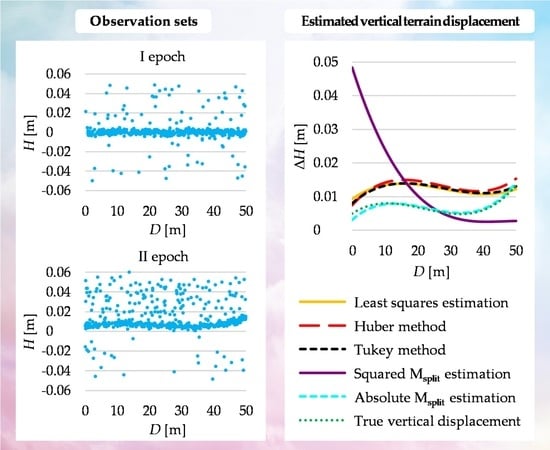
The generated observation sets for these variants are presented in Figure 1 (Variants I–III) and Figure 2 (Variants IV–VI).

Let us estimate the third-degree polynomial coefficients in each epoch separately by applying SMS, AMS estimations, and, for comparison, the conventional methods, namely the LS, Huber, and Tukey methods. Note that in the case of M_split estimation, we always obtain two competitive solutions in each epoch. Considering the terms of the case at hand (namely, the terrain profile estimation), one can choose the solution, namely the polynomial, whose graph is located lower (as it is recommended in such a case in [36,40]). This works effectively when only positive gross errors occur but not if only negative gross errors disturb the observation sets. Hence, one can choose the polynomial, which is better fitted in most TLS points as the M_split solution corresponding to the terrain profile (choosing such m for which ${\displaystyle \sum _{i=1}^n{v}_{i(m)}^2}$ in SMS estimation or ${\displaystyle \sum _{i=1}^n\left|v_{i(m)}^{}\right|}$ in AMS estimation is lower—that approach is applied here). Such a choice would be questionable when the number of terrain observations is smaller than the number of other disturbing observations. Then, the correct solution choice would depend on the analyst’s experience. Note that the second solutions obtained during M_split estimation describe the location of outliers in general. They are of no interest in the problem at hand; hence, they are omitted.

The estimates of the polynomial coefficients allow us to compute each epoch’s estimated profile heights (every meter). One can obtain the terrain displacements at the chosen points by subtracting the respective point heights. Figure 3 presents the height differences between the measurement epochs, namely the estimation results obtained for all variants and methods applied when the observations from two measurement epochs are processed separately. All estimation methods provide similar and correct results for the two first variants. The differences between the methods appear in the four subsequent variants (see Section 4).

The graphical interpretation only provides a general comparison between the methods. The minor differences between the estimation results (especially in Variants I and II) are unnoticeable. In order to compare the results, let us assess how the estimated displacements fit into the theoretical simulated ones. One can evaluate the accuracy of the estimated terrain displacement by using the root-mean-square deviation $RMSD\left(\mathsf{\Delta }\hat{H}\right)$ computed in the following way [36]:

$$RMSD\left(\mathsf{\Delta }\hat{H}\right)=\sqrt{\frac{{\displaystyle \sum _{j=0}^{50}{\left(\mathsf{\Delta }{\hat{H}}_j-\mathsf{\Delta }{H}_j\right)}^2}}{51}}$$

(16)

where $\mathsf{\Delta }{\hat{H}}_j$—estimated displacements, ΔH_j—simulated displacements; displacements are calculated for distances $D_j=j\cdot 1 \mathrm{m}$ $\left(j=0, ..., 50\right)$. One can take more points in the formula of Equation (16); however, the results would be comparable.

The computed RMSDs for all variants are presented in

Table 1. RMSDs of estimated displacements (mm).

Variant	LS	Huber	Tukey	SMS	AMS
I	0.29	0.33	0.30	0.50	0.43
II	0.38	0.20	0.13	0.25	0.15
III	5.62	5.63	5.68	10.13	0.16
IV	1.21	0.30	0.76	18.35	0.26
V	1.24	0.23	1.07	6.54	0.11
VI	5.48	6.27	5.51	14.73	0.62

.

In many practical applications of M_split estimation, we apply only one observation set, namely the set consisting of two (or more) observation groups. Such an approach is natural for M_split estimation and advisable in many surveying problems [15,36,51,52]. It could also be involved in deformation analysis [53,54]. Let us apply such an approach to process the combined simulated TLS data in each variant (presented in the right panels of Figure 1 and Figure 2). In such a case, the polynomial coefficients are estimated in one estimation process. One of the two obtained competitive solutions directly refers to the first measurement epoch, while the other refers to the second one. Thus, this time we do not neglect any M_split estimates (as was the case in the previous approach). Figure 4 presents the estimated vertical terrain displacement from the combined observation set.

AMS estimation only provides correct results in Variants II and IV. The displacements estimated by using the SMS method are distant from the theoretical values in all variants. Generally, the estimated vertical terrain displacements obtained from the combined observation set are worse than those obtained from processing two separate observation sets. Once again, we can supplement the graphical analysis by evaluating the accuracy of the estimated terrain displacement.

Table 2. RMSDs of estimated displacements from the combined observation set (mm).

Variant	SMS	AMS
I	15.17	10.88
II	26.32	1.82
III	28.87	21.18
IV	27.30	0.83
V	24.06	10.97
VI	25.47	17.06

presents the RMSDs of the fit of the estimated displacements to the simulated ones.

The obtained values indicate that the estimation based on the combined observation sets provides much less accurate results than when processing each epoch’s observations separately. It may seem that SMS and AMS estimation cannot handle outliers. However, one may notice that the results obtained in Variant I are also very poor. This means that the magnitude of the terrain displacements is not enough to make the “separation” between regular observations from the first and second epochs easily detectable.

4. Discussion

Considering results from the first approach presented, and based on the processing data from different epochs separately, one can notice that LS estimation provides the best results if there are no outliers. However, the results of robust M-estimation variants are only marginally worse. The results of M_split estimation variants are also comparable (especially for AMS estimation). Interestingly, LS estimation shows robustness against outliers in Variants II or IV and even V. This stems from the outlier distribution and shares within the data sets. Such observations are spread over the whole profile randomly and uniformly. The terrain profiles obtained in each epoch themselves, which are not presented here, are significantly disturbed by outliers; however, after subtracting the results from two epochs, such an effect is eliminated. In Variant II, other methods also seem to not be sensitive to outliers. On one hand, the low share of outliers is not an issue for robust M-estimation; on the other hand, M_split estimation can distinguish two groups of observations (regular and outlying ones) in each measurement epoch.

In the case of Variants IV and V, the best results are obtained for the Huber method and AMS estimation. The accuracies for these two methods are significantly higher than for the remaining methods considered here. LS estimation, as well as the Tukey method, provide marginally worse outcomes. The estimated vertical terrain displacements obtained by using SMS estimation are not correct. One can say that this method cannot handle the shares of outliers (Variant IV) and the combination of positive and negative outliers (Variant V). The significant differences between the methods are in Variants III and VI, wherein only the AMS estimation provides correct results. The AMS estimates are significantly more accurate than the estimates of the other considered methods. LS estimation and SMS estimation are not able to handle the different shares of outlying observations in both measurement epochs.

In contrast, the robust M-estimation cannot handle 30% of outliers at the second measurement epoch. Thus, AMS estimation predominates over conventional robust M-estimation for a higher percentage of outliers. One should also note that AMS estimation overperforms SMS estimation in such cases. Additionally, in the other papers, it was proven that AMS estimation predominates SMS estimation in different applications [36,41].

The numerical tests showed that the second possible approach, namely processing one combined observation set, should not be used in the cases of the observation sets simulated here. As mentioned, the separation between the subsets is not so evident; hence, M_split estimation variants could not separate the subsets successfully. Additionally, at distances from 30 m to 40 m, the terrain profiles from both epochs are very close to each other. Thus, it is difficult to “determine” whether the profiles cross or if one is always above the other (such a disadvantage does not appear in processing each epoch separately). In conclusion, the estimation process is disturbed, resulting in the low accuracy of the outcomes. The exception is the results for AMS estimation for Variants II and IV, which seem rather satisfactory. This results from the location of outliers (they are all positive or all negative). Thus, all outliers are assigned to the regular observations from the second epoch (Variant II) or the first one (Variant IV), and AMS estimations “have” less trouble with distinguishing observations from different epochs (especially at the distances 30–40 m).

What if the terrain displacements were more significant (compared to the measurement accuracy)? Would the M_split estimation provide better results? In order to verify that supposition, we change the observation sets in Variants I, II, and VI by shifting all observations in the second epoch by 5 cm. Then, estimating the terrain displacements by using one combined set, one can obtain the following accuracies: in Variant I, 0.20 mm for SMS estimation and 0.32 mm for AMS estimation; in Variant III, 34.62 mm for SMS estimation and 0.91 mm for AMS estimation; in Variant VI, 37.20 mm for SMS estimation and 0.93 mm for AMS estimation. One can say that when there are no outliers in the observation set, the obtained results are much better; they are even more accurate than the results from separated processing. This is not surprising since the processed set contains two very distinctive subsets; thus, M_split estimation has no problem isolating subsets. However, if outliers occur, only AMS estimation results become more accurate than before. The outcomes confirm the advantages of AMS estimation over SMS estimation in this paper’s context. Analyzing the obtained accuracies, one can say that even if the terrain moved more significantly, it is more advisable to process data from different measurement epochs separately.

The methods described here can also be used for other TLS technique applications. A similar analysis can concern, e.g., a beam deflection or deformation under a changing load [40,50] or landslides [55]. In the case of massive landslides, when the terrain changes significantly, one may consider the second approach presented here.

Here, we focus on the method’s sensitivity to outliers when TLS data are applied in deformation analysis. Thus, it was necessary to know the real surface and its deformation, hence the necessity of data simulation. The applications of M_split estimation to determine terrain profiles or geodetic network deformation using real data can be found in other papers [36,40,53,56].

5. Conclusions

M_split estimation is a contemporary method dedicated to processing observation sets consisting of two (or more) unrecognized observation groups. Such data are characteristic of TLS or, more generally, LiDAR measurements. This paper showed that the method in question could be applicable in analyzing vertical terrain displacement determined from TLS data. The presented example shows that such an approach seems advisable when the share of outlying observations is high, which makes the application of robust M-estimation unsuccessful. One should consider the application of AMS estimation in such a context.

M_split estimation always provides at least two competitive versions of the parameter vector (this depends on the declared a priori number of groups). Thus, one should know which version responds to the terrain profile (or surface). Considering this paper’s context, the latter parameter version that describes possible outliers is of no interest to us. In the case of TLS data, we almost always know which estimated profile (or surface) from two competitive versions we should choose as the outcome. For example, we almost always choose the lower estimated profile as the one which concerns the terrain profile. The exception is the case wherein only negative outliers occur. Negative outliers usually result when laser beams reflect several times before they are detected [11]; hence, one can suppose that such outliers are more likely in ALS techniques, especially in urban areas. When applying the TLS technique in terrain profile determination, one should expect positive outliers to predominate over negative ones. Thus, the choice of a lower estimated profile seems proper from the practical point of view (in the case of any doubt, one can also apply the approach given in the numerical example).

This paper also verifies two approaches to process TLS data from two epochs by applying M_split estimation. Doubtless, processing observation sets from both epochs separately is a much better approach than using the combined observation set if one does not know the magnitude of a terrain displacement.

References

- Gordon, S.J.; Lichti, D.D. Modeling Terrestrial Laser Scanner Data for Precise Structural Deformation Measurement. J. Surv. Eng. 2007, 133, 72–80. [Google Scholar] [CrossRef]
- Wang, C.; Hsu, P.-H. Building Detection and Structure Line Extraction from Airborne LiDAR Data. J. Photogramm. Remote Sens. 2007, 12, 365–379. [Google Scholar]
- Spaete, L.P.; Glenn, N.F.; Derryberry, D.R.; Sankey, T.T.; Mitchell, J.J.; Hardegree, S.P. Vegetation and Slope Effects on Accuracy of a LiDAR-Derived DEM in the Sagebrush Steppe. Remote Sens. Lett. 2011, 2, 317–326. [Google Scholar] [CrossRef]
- Rodríguez-Gonzálvez, P.; Jiménez Fernández-Palacios, B.; Muñoz-Nieto, Á.L.; Arias-Sanchez, P.; Gonzalez-Aguilera, D. Mobile LiDAR System: New Possibilities for the Documentation and Dissemination of Large Cultural Heritage Sites. Remote Sens. 2017, 9, 189. [Google Scholar] [CrossRef] [Green Version]
- Crespo-Peremarch, P.; Tompalski, P.; Coops, N.C.; Ruiz, L.Á. Characterizing Understory Vegetation in Mediterranean Forests Using Full-Waveform Airborne Laser Scanning Data. Remote Sens. Environ. 2018, 217, 400–413. [Google Scholar] [CrossRef]
- Matwij, W.; Gruszczyński, W.; Puniach, E.; Ćwiąkała, P. Determination of Underground Mining-Induced Displacement Field Using Multi-Temporal TLS Point Cloud Registration. Measurement 2021, 180, 109482. [Google Scholar] [CrossRef]
- Haddad, D.E.; Akçiz, S.O.; Arrowsmith, J.R.; Rhodes, D.D.; Oldow, J.S.; Zielke, O.; Toké, N.A.; Haddad, A.G.; Mauer, J.; Shilpakar, P. Applications of Airborne and Terrestrial Laser Scanning to Paleoseismology. Geosphere 2012, 8, 771–786. [Google Scholar] [CrossRef] [Green Version]
- Walicka, A.; Pfeifer, N. Automatic Segmentation of Individual Grains from a Terrestrial Laser Scanning Point Cloud of a Mountain River Bed. IEEE J. Sel. Top. Appl. Earth Obs. Remote Sens. 2022, 15, 1389–1410. [Google Scholar] [CrossRef]
- Mücke, W.; Deák, B.; Schroiff, A.; Hollaus, M.; Pfeifer, N. Detection of Fallen Trees in Forested Areas Using Small Footprint Airborne Laser Scanning Data. Can. J. Remote Sens. 2013, 39, S32–S40. [Google Scholar] [CrossRef]
- Kuzia, K. Application of airborne laser scanning in monitoring of land subsidence caused by underground mining expoloitation. Geoinform. Pol. 2016, 2016, 7–13. [Google Scholar] [CrossRef]
- Matkan, A.A.; Hajeb, M.; Mirbagheri, B.; Sadeghian, S.; Ahmadi, M. Spatial Analysis for Outlier Removal from LiDAR Data. In Proceedings of the The International Archives of the Photogrammetry, Remote Sensing and Spatial Information Sciences, Tehran, Iran, 15–17 November 2014; Copernicus GmbH: Göttingen, Germany, 2014; Volume XL-2-W3, pp. 187–190. [Google Scholar]
- Carrilho, A.C.; Galo, M.; Santos, R.C. Statistical Outlier Detection Method for Airborne LiDAR Data. In Proceedings of the ISPRS TC I Mid-term Symposium “Innovative Sensing—From Sensors to Methods and Applications”, Karlsruhe, Germany, 10–12 October 2018; Volume XLII–1, pp. 87–92. [Google Scholar] [CrossRef]
- Zhang, K.; Chen, S.-C.; Whitman, D.; Shyu, M.-L.; Yan, J.; Zhang, C. A Progressive Morphological Filter for Removing Nonground Measurements from Airborne LIDAR Data. IEEE Trans. Geosci. Remote Sens. 2003, 41, 872–882. [Google Scholar] [CrossRef] [Green Version]
- Chen, Z.; Gao, B.; Devereux, B. State-of-the-Art: DTM Generation Using Airborne LIDAR Data. Sensors 2017, 17, 150. [Google Scholar] [CrossRef] [PubMed] [Green Version]
- Błaszczak-Bąk, W.; Janowski, A.; Kamiński, W.; Rapiński, J. Application of the Msplit Method for Filtering Airborne Laser Scanning Data-Sets to Estimate Digital Terrain Models. Int. J. Remote Sens. 2015, 36, 2421–2437. [Google Scholar] [CrossRef]
- Kraus, K.; Pfeifer, N. Determination of Terrain Models in Wooded Areas with Airborne Laser Scanner Data. ISPRS J. Photogramm. Remote Sens. 1998, 53, 193–203. [Google Scholar] [CrossRef]
- Schnabel, R.; Wahl, R.; Klein, R. Efficient RANSAC for Point-Cloud Shape Detection. Comput. Graph. Forum 2007, 26, 214–226. [Google Scholar] [CrossRef]
- Tóvári, D.; Pfeifer, N. Segmentation Based Robust Interpolation—A New Approach to Laser Data Filtering. Int. Arch. Photogramm. Remote Sens. Spat. Inf. Sci. 2012, 36, 79–84. [Google Scholar]
- Nguyen, A.; Le, B. 3D Point Cloud Segmentation: A Survey. In Proceedings of the 2013 6th IEEE Conference on Robotics, Automation and Mechatronics (RAM), Manila, Philippines, 12–15 November 2013; pp. 225–230. [Google Scholar]
- Nurunnabi, A.; Belton, D.; West, G. Robust Statistical Approaches for Local Planar Surface Fitting in 3D Laser Scanning Data. ISPRS J. Photogramm. Remote Sens. 2014, 96, 106–122. [Google Scholar] [CrossRef] [Green Version]
- Li, L.; Yang, F.; Zhu, H.; Li, D.; Li, Y.; Tang, L. An Improved RANSAC for 3D Point Cloud Plane Segmentation Based on Normal Distribution Transformation Cells. Remote Sens. 2017, 9, 433. [Google Scholar] [CrossRef] [Green Version]
- Zhao, R.; Pang, M.; Liu, C.; Zhang, Y. Robust Normal Estimation for 3D LiDAR Point Clouds in Urban Environments. Sensors 2019, 19, 1248. [Google Scholar] [CrossRef] [Green Version]
- Berber, M.; Hekimoglu, S. What Is the Reliability of Conventional Outlier Detection and Robust Estimation in Trilateration Networks? Surv. Rev. 2003, 37, 308–318. [Google Scholar] [CrossRef]
- Lehmann, R.; Scheffler, T. Monte Carlo-Based Data Snooping with Application to a Geodetic Network. J. Appl. Geod. 2011, 5, 123–134. [Google Scholar] [CrossRef]
- Rofatto, V.F.; Matsuoka, M.T.; Klein, I.; Roberto Veronez, M.; da Silveira, L.G. A Monte Carlo-Based Outlier Diagnosis Method for Sensitivity Analysis. Remote Sens. 2020, 12, 860. [Google Scholar] [CrossRef] [Green Version]
- Hodges, J.L.; Lehmann, E.L. Estimates of Location Based on Rank Tests. Ann. Math. Statist. 1963, 34, 598–611. [Google Scholar] [CrossRef]
- Huber, P.J.; Ronchetti, E.M. Robust Statistics, 2nd ed.; John Wiley & Sons, Ltd.: Hoboken, NJ, USA, 2009; ISBN 978-0-470-43469-7. [Google Scholar]
- Baarda, W. A Testing Procedure for Use in Geodetic Networks; Publications on Geodesy 9; Rijkscommissie voor Geodesie: Delft, The Netherlands, 1968; Volume 2, ISBN 978 90 6132 209. [Google Scholar]
- Pope, A.J. The Statistics of Residuals and the Outlier Detection of Outliers; NOAA Technical Report; National Geodetic Survey: Rockville, MD, USA, 1976; Volume NGS 1.
- Gui, Q.; Zhang, J. Robust Biased Estimation and Its Applications in Geodetic Adjustments. J. Geod. 1998, 72, 430–435. [Google Scholar] [CrossRef]
- Duchnowski, R. Hodges-Lehmann Estimates in Deformation Analyses. J. Geod. 2013, 87, 873–884. [Google Scholar] [CrossRef] [Green Version]
- Ge, Y.; Yuan, Y.; Jia, N. More Efficient Methods among Commonly Used Robust Estimation Methods for GPS Coordinate Transformation. Surv. Rev. 2013, 45, 229–234. [Google Scholar] [CrossRef]
- Lehmann, R. On the Formulation of the Alternative Hypothesis for Geodetic Outlier Detection. J. Geod. 2013, 87, 373–386. [Google Scholar] [CrossRef] [Green Version]
- Wiśniewski, Z. Estimation of Parameters in a Split Functional Model of Geodetic Observations (Msplit Estimation). J. Geod. 2009, 83, 105–120. [Google Scholar] [CrossRef]
- Wiśniewski, Z. Msplit(q) Estimation: Estimation of Parameters in a Multi Split Functional Model of Geodetic Observations. J. Geod. 2010, 84, 355–372. [Google Scholar] [CrossRef]
- Wyszkowska, P.; Duchnowski, R.; Dumalski, A. Determination of Terrain Profile from TLS Data by Applying Msplit Estimation. Remote Sens. 2021, 13, 31. [Google Scholar] [CrossRef]
- Janowski, A.; Rapiński, J. M-Split Estimation in Laser Scanning Data Modeling. J. Indian Soc. Remote Sens. 2013, 41, 15–19. [Google Scholar] [CrossRef]
- Janowski, A. The Circle Object Detection with the Use of Msplit Estimation. E3S Web Conf. 2018, 26, 00014. [Google Scholar] [CrossRef] [Green Version]
- Janicka, J.; Rapiński, J.; Błaszczak-Bąk, W.; Suchocki, C. Application of the Msplit Estimation Method in the Detection and Dimensioning of the Displacement of Adjacent Planes. Remote Sens. 2020, 12, 3203. [Google Scholar] [CrossRef]
- Wyszkowska, P.; Duchnowski, R. Processing TLS Heterogeneous Data by Applying Robust Msplit Estimation. Measurement 2022, 197, 111298. [Google Scholar] [CrossRef]
- Wyszkowska, P.; Duchnowski, R. Msplit Estimation Based on L1 Norm Condition. J. Surv. Eng. 2019, 145, 04019006. [Google Scholar] [CrossRef]
- Kargoll, B. Comparison of Some Robust Parameter Estimation Techniques for Outlier Analysis Applied to Simulated GOCE Mission Data. In Proceedings of the Gravity, Geoid and Space Missions; Jekeli, C., Bastos, L., Fernandes, J., Eds.; Springer: Berlin/Heidelberg, Germany, 2005; pp. 77–82. [Google Scholar]
- Chang, X.-W.; Guo, Y. Huber’s M-Estimation in Relative GPS Positioning: Computational Aspects. J. Geod. 2005, 79, 351–362. [Google Scholar] [CrossRef] [Green Version]
- Labant, S.; Weiss, G.; Kukučka, P. Robust Adjustment of a Geodetic Network Measured by Satellite Technology in the Dargovských Hrdinov Suburb. Acta Montan. Slovaca 2014, 16, 229–237. [Google Scholar]
- Yang, Y. Robust Estimation for Dependent Observations. Manuscr. Geod. 1994, 19, 10–17. [Google Scholar]
- Wiśniewski, Z. Total Msplit Estimation. J. Geod. 2022, 96, 82. [Google Scholar] [CrossRef]
- Wyszkowska, P.; Duchnowski, R. Iterative Process of Msplit(q) Estimation. J. Surv. Eng. 2020, 146, 06020002. [Google Scholar] [CrossRef]
- Forlani, G.; Nardinocchi, C. Adaptive Filtering of Aerial Laser Scanning Data. Int. Arch. Photogramm. Remote Sens. Spat. Inf. Sci. 2007, 36, 130–135. [Google Scholar]
- Costantino, D.; Angelini, M.G. Production of DTM Quality by TLS Data. Eur. J. Remote Sens. 2013, 46, 80–103. [Google Scholar] [CrossRef] [Green Version]
- Cabaleiro, M.; Riveiro, B.; Arias, P.; Caamaño, J.C. Algorithm for Beam Deformation Modeling from LiDAR Data. Measurement 2015, 76, 20–31. [Google Scholar] [CrossRef]
- Nowel, K. Squared Msplit(q) S-Transformation of Control Network Deformations. J. Geod. 2019, 93, 1025–1044. [Google Scholar] [CrossRef]
- Guo, Y.; Li, Z.; He, H.; Zhang, G.; Feng, Q.; Yang, H. A Squared Msplit Similarity Transformation Method for Stable Points Selection of Deformation Monitoring Network. Acta Geod. Cartogr. Sin. 2020, 49, 1419–1429. [Google Scholar] [CrossRef]
- Zienkiewicz, M.H. Determination of Vertical Indicators of Ground Deformation in the Old and Main City of Gdansk Area by Applying Unconventional Method of Robust Estimation. Acta Geodyn. Geomater. 2015, 12, 249–257. [Google Scholar] [CrossRef] [Green Version]
- Zienkiewicz, M.H. Deformation Analysis of Geodetic Networks by Applying Msplit Estimation with Conditions Binding the Competitive Parameters. J. Surv. Eng. 2019, 145, 04019001. [Google Scholar] [CrossRef]
- Lian, X.; Hu, H. Terrestrial Laser Scanning Monitoring and Spatial Analysis of Ground Disaster in Gaoyang Coal Mine in Shanxi, China: A Technical Note. Environ. Earth Sci 2017, 76, 287. [Google Scholar] [CrossRef]
- Zienkiewicz, M.H.; Hejbudzka, K.; Dumalski, A. Multi Split Functional Model of Geodetic Observations in Deformation Analyses of the Olsztyn Castle. Acta Geodyn. Geomater. 2017, 14, 195–204. [Google Scholar] [CrossRef]
Figure 1.
Observation sets for Variants I–III.
Figure 2.
Observation sets for Variants IV–VI.
Figure 3.
Estimated vertical terrain displacement for different variants.
Figure 4.
Estimated vertical terrain displacement (from the combined observation set) for different variants.