
An Integrated InSAR and GNSS Approach to Monitor Land Subsidence in the Po River Delta (Italy)
by
 , , and
Massimo Fabris
1,
Mattia Battaglia
2,
Xue Chen
3,4,5,*,
Andrea Menin
1,
Michele Monego
1 and
Mario Floris
4
1
Department of Civil, Environmental and Architectural Engineering, University of Padua, 35131 Padua, Italy
2
Spektra S.R.L.—A Trimble Company, Via Pellizzari 23/A, 20871 Vimercate, Italy
3
National Institute of Natural Hazards, Ministry of Emergency Management of China, Beijing 100085, China
4
Department of Geosciences, University of Padua, 35131 Padua, Italy
5
School of Land Science and Technology, China University of Geosciences, Beijing 100083, China
*
Author to whom correspondence should be addressed.
Remote Sens. 2022, 14(21), 5578; https://doi.org/10.3390/rs14215578
Submission received: 2 September 2022
/
Revised: 20 October 2022
/
Accepted: 26 October 2022
/
Published: 4 November 2022
(This article belongs to the Special Issue Ground and Structural Deformations Monitoring Systems Integrating Remote Sensing and Ground-Based Data)
Abstract
:Land subsidence affects many areas of the world, posing a serious threat to human structures and infrastructures. It can be effectively monitored using ground-based and remote sensing techniques, such as the Global Navigation Satellite System (GNSS) and Interferometric Synthetic Aperture Radar (InSAR). GNSS provides high precision measurements, but in a limited number of points, and is time-consuming, while InSAR allows one to obtain a very large number of measurement points, but only in areas characterized by a high and constant reflectivity of the signal. The aim of this work is to propose an approach to combine the two techniques, overcoming the limits of each of them. The approach was applied in the Po River Delta (PRD), an area located in Northern Italy and historically affected by land subsidence. Ground-based GNSS data from three continuous stations (CGNSS) and 46 non-permanent sites (NPS) measured in 2016, 2018, and 2020, and Sentinel-1 and COSMO-SkyMed SAR data acquired from 2016 to 2020, were considered. In the first phase of the method, InSAR processing was calibrated and verified through CGNSS measurements; subsequently, the calibrated interferometric data were used to validate the GNSS measurements of the NPS. In the second phase, the datasets were integrated to provide an efficient monitoring system, extracting high-resolution deformation maps. The results showed a good agreement between the different sources of data, a high correlation between the displacement rate and the age of the emerged surfaces composed of unconsolidated fine sediments, and high land subsidence rates along the coastal area (up to 16–18 mm/year), where the most recent deposits outcrop. The proposed approach makes it possible to overcome the disadvantages of each technique by providing more complete and detailed information for a better understanding of the ongoing phenomenon.
1. Introduction
Ground deformation due to land subsidence affects many areas around the world [1]. This phenomenon increases the risk of flooding along with transitional environments, such as river deltas, which are often characterized by a large population and extensive economic activities [2,3]. The consequences of environmental degradation caused by land subsidence are related to coastline and surface changes, services interruption, buildings damage, salinization, and flooding of large areas [4,5,6,7,8,9,10]. In the next few years, rising sea level caused by climatic changes could dramatically increase the negative impact of land subsidence [11,12,13].
Monitoring areas affected by land subsidence is crucial for the implementation of risk mitigation strategies. Various techniques can be used to carry out monitoring activities. In the past, only ground-based precise geometric leveling was used, while at present time the development of high-precision remote sensing techniques, such as InSAR, and ground-based GNSS methodology, can integrate and/or replace the leveling measurements that require high costs and very long execution times. The integration of the two techniques can be used to align the remote sensing data with ground-based measurements, validate each other, and overcome the limits of each methodology by increasing the spatial and the temporal resolution together with the cost-effectiveness of both approaches [14].
Many authors have combined InSAR and GNSS measurements in the management and monitoring of different phenomena. Magnússon et al. [15] integrated InSAR from ERS-1/2 satellites with CGPS measurements to detect localized anomalies in the vertical ice motion of an outlet glacier of Vatnajökull (Iceland). Cheng et al. [16] compared atmospheric delay between GPS and InSAR in both differential and pseudoabsolute modes, demonstrating the potentiality to correct atmospheric errors in SAR interferometry with high-precision GPS meteorological products. Bovenga et al. [17] applied different space-borne SAR data (both in the C-band and in the X-band), and in situ GNSS measurements for the deformation monitoring of the Assisi landslide (Italy). Tapete et al. [18] applied InSAR together with measurements collected by real-time kinematic (RTK) GPS surveying for the structural motion detection of the Roman Aqueducts in Rome (Italy). Gudmundsson et al. [19] used aircraft-based altimetry, satellite photogrammetry, radar interferometry, ground-based GPS, the evolution of seismicity, radioecho soundings of ice thickness, ice flow modeling, and geobarometry to describe and analyze the spatial evolution of land subsidence in the Bárdarbunga caldera volcano (Iceland). Wilkinson et al. [20] used low-cost GNSS receivers located in the Mt. Vettore–Mt. Bove fault system recording the near-field coseismic displacement during the 30 October 2016 Mw 6.6 earthquake (Central Italy) and observing a clear temporal and spatial link between the near-field GNSS record and InSAR, far-field GPS data, regional measurements from the Italian Strong Motion and National Seismic networks, and field measurements of surface ruptures. Saleh and Becker [21] estimated the vertical motion in the Nile Delta (Egypt) through a persistent scatterer (PS) InSAR analysis, using the available CGPS stations to validate the obtained subsidence rates. Farolfi et al. [22] performed the datum alignment of the InSAR products using precise velocity fields derived from the CGNSS stations to provide a detailed map of the movement of the ground in Italy. Benetatos et al. [23] used InSAR and GNSS for a fully integrated and multidisciplinary geological, fluid-flow, and geomechanical numerical modeling approach, developed to reproduce the main geometrical and structural features of the poromechanics processes induced by the storage operations in the Po Plain area (Italy). Grgić et al. [24] analyzed the vertical land motion of the Dubrovnik area (Croatia) using Sentinel-1 InSAR data, continuous GNSS observations, and differences in the sea level change obtained from available satellite altimeter missions and tide gauge measurements. Cenni et al. [14] integrated InSAR Sentinel-1 data with aerial photogrammetry and CGNSS in monitoring the Patigno landslide (Italy). Chen et al. [25] combined InSAR data from Sentinel-1A/B satellites with GNSS multitemporal measurements for the validation of the remote sensing data and the monitoring of ground and structural deformations of buildings located in the Rovegliana landslide (Italy). Maltese et al. [8] used Sentinel-1 images, Landsat 8 thermal infrared sensor (TIRS) images, and CGNSS stations for interpreting the motion of the top of a dam (Italy). Mancini et al. [26] provided a full interferometry processing chain based on dual orbit Sentinel-1 SAR data combined with open source routines from the Sentinel Application Platform (SNAP), Stanford Method for Persistent Scatterers (StaMPS), and additional routines introduced by the authors, using data from CGNSS stations to provide a global reference frame for line-of-sight projected velocities and to validate velocity maps after the decomposition analysis. Many other applications integrating InSAR and GNSS data are available in the literature.
Despite the numerous previous studies, the integration between interferometric data and GNSS can still be improved, thanks to the ever-increasing availability of remote sensing data and the refinement of processing techniques. In the above-mentioned works, the comparison between the two techniques was generally performed using: (i) single SAR datasets, in terms of band and/or resolution; (ii) specific GNSS observations (continuous or non-permanent); (iii) a limited number of GNSS points, making the comparison not fully explored. For these reasons, in this study, different InSAR data: Sentinel-1 and COSMO-SkyMed (CSK), and different GNSS observations (3 CGNSS and 46 NPS GNSS sites) are used, and the comparison between GNSS and InSAR techniques is investigated in detail. Moreover, the availability of 49 GNSS points makes the process statistically stronger. Only after comparison, calibration, and validation, can the satellite- and ground-based data be fully integrated to provide the complete monitoring system of the study area.
In detail, InSAR data derived from Sentinel-1 from 1 October 2016 to 27 December 2020 and CSK from 25 May 2017 to 5 August 2020 were combined with the PODELNET (PO DELta NETwork) GNSS network (surveys performed in 2016, 2018, and 2020) to provide a land subsidence monitoring system of the PRD. The study area, located in northeastern Italy (Figure 1), was characterized in the past by high land subsidence rates, and today the phenomenon, even though it is reduced, is still ongoing [27,28,29,30,31]. In the first phase, data gathered from CGNSS stations (i.e., coordinates and velocities) were used to calibrate InSAR results and process PODELNET measurements (Figure 2); subsequently, space and ground-based data were compared to evaluate: (i) uncertainties, (ii) local deformation effects, and (iii) outliers. Finally, the datasets were integrated, providing the deformation pattern of the study area.
2. The Study Area
The PRD is a complex ecosystem with an extension of about 400 km2 in North-East Italy, where the Po River flows into the Adriatic Sea. It is the result of natural sedimentary processes linked to human activities, such as filling the wetlands area and engineering endeavors [32]. A large part of the delta is characterized mainly by reclaimed territories and is a complex system of shallow water bodies.
This area is inserted in the broad foreland region located between the NE-verging Northern Apennine to the south and the Venetian Plain, limited by the SSE-verging Eastern South-Alpine, to the north. The sedimentary infill is composed of terrigenous Apennine and Alpine sediments up to 2000 m thick, accumulated in different environments during the Pliocene and the Quaternary, mostly made of sandy and silty-clay layers of alluvial and marine deposition. Despite the different thickness, the stratigraphy of the Quaternary soils is quite similar to the well-developed freshwater multi-aquifer systems that are located in the upper 500–600 m. Semi-confined aquifers occur within the Holocene deposits where clayey and sandy layers are discontinuous and heterogeneous [28,31,33].
Land subsidence in this area is due to natural and anthropogenic factors: the natural component is strongly correlated with the age of the highly compressible Holocene deposits that compose the shallowest 30–40 m of the sedimentary sequence [28] and tectonic movements [34,35], and is characterized by rates in the order of 2–4 mm/year [28,33,34]. In terms of contribution to the land subsidence rate, it can be considered that the long-term natural factors (tectonics and glacio-isostasy) are not so crucial, while the natural compaction of recent alluvial fine-grained deposits, which increases from the mainland toward the sea, has a major importance [36].
The anthropogenic component is linked to the extensive exploitation of non-confined, semi-confined, and confined aquifers [37] and can reach velocities from tens to hundreds of mm/year (for more details see [14]).
Currently, a large portion of PRD is below the mean sea level and it has a very low sediment supply due to artificial levees built to prevent flooding [38]. The extensive exploitation of the multi-aquifers system of the Po Plain for anthropic (industrial and agricultural) uses after the Second World War, and the methane–water withdrawals from onshore and offshore reservoirs, led to a significant increase in subsidence in the 1950s. Many researchers [28,29,30,39,40] have estimated subsidence rates of up to 300 mm/year in the period from 1950 to 1957 in the Po plain and PRD, by using geometric leveling measurements. Therefore, at the beginning of the 1960s, the Italian Government suspended the anthropogenic withdrawals leading to a progressive benefit, highlighted by vertical settlement rates of about 30 mm/year from 1962 to 1974 [29,41]. From the late 1970s to the present time, land subsidence rates have continued to decline to values less than 10 mm/year [4,14,27,36,40,42,43], demonstrating the successful policies applied 50 years ago to reduce the effects of anthropogenic factors.
3. Materials and Methods
3.1. SAR Data and Processing
The SAR data used in this study included X-band CSK and C-band Sentinel-1 images. CSK has a short wavelength (3.1 cm) and a higher spatial resolution (about 3 m), and thus it can achieve high-density and precise measurements in monitoring buildings, structures, and infrastructures. Sentinel-1 satellites have provided free accessible images since 2014. The longer C-band wavelength (5.55 cm) satisfy the demand for monitoring a larger land subsidence rate. In addition, the wide width of the swath (250 km) makes it easy to find a stable point as a reference point.
Two stacks of CSK data covered the study area. The east stack (E) included 128 images acquired from 13 March 2012 to 10 August 2020 from descending orbit in the Stripmap Himage mode at horizontal transmit and horizontal receive (HH) polarization, with an incidence angle of 34° and a heading angle of 194°. The west (W) one included 57 images acquired from 25 May 2017 to 5 August 2020, in the same mode and polarization, with an incidence angle of 26° and a heading angle of 194°. The spatial resolution was 3 × 3 m.
Sentinel-1 dataset consisted of 180 images spanning from 1 October 2016 to 27 December 2020, acquired along the descending orbit 95, in terrain observation with progressive scans (TOPS) mode at vertical transmit and vertical receive (VV) polarization, with an incidence angle of 39°, a heading angle of 194°, and about a 10 × 5 m spatial resolution.
The CSK images were connected to a reference image dated 21 February 2016 (east stack) and 25 May 2017 (west stack), respectively. The maximum temporal baseline was 1632 days, and the maximum spatial baseline was 1786 m for the east stack, and 1168 days and 1761 m for the west stack. All available CSK data in the east stack from 13 March 2012 to 10 August 2020, were processed. Then, the time series deformation in the period 12 June 2016–10 August 2020 (overlapping the PODELNET GNSS surveys) was extracted from the long-term time series displacement and fitted into a linear model to obtain the linear deformation rate. Sentinel-1 images were connected to the reference image dated 7 January 2019, with a maximum temporal baseline of 828 days and a maximum spatial baseline of 178.2 m (Figure 3).
Multi-temporal InSAR (MT-InSAR) techniques have become a widely used tool for monitoring land surface deformation. The two main classes of MT-InSAR techniques are PS [44,45,46] and small baseline subsets (SBAS) [47]. The PS technique is usually used in urban areas to identify buildings and man-made structures as PS candidates. All the images are referenced to one primary image. The deformation rate and height correction are usually solved by a linear function. The SBAS technique establishes points by multi-look processing, identifying points both in urban and nonurban areas [48]. The connection is built according to small temporal and spatial baselines to maintain good coherence. Then, singular value decomposition (SVD) is applied to calculate the linear rate of deformation. The atmospheric phase is regarded as spatially correlated and temporally uncorrelated and filtered in spatial scale.
In this case study, the PS technique was adopted, because (i) the land subsidence rate in this area is near-linear; (ii) the low urbanization with a large area of lagoons has a very low coherence even after multi-look processing using the SBAS technique.
PS processing was achieved by applying the interferometric point target analysis (IPTA) implemented in GAMMA software (https://www.gamma-rs.ch/software, accessed on 1 September 2022) [36,49]. The IPTA steps are as follows. A single reference interferometric network is built considering a primary image in the center (or at the beginning) of the period. The PS candidates are identified by considering points with low spectral diversity and low temporal backscatter variability. For spectral diversity, the minimum average spectral correlation is usually set to 0.4, and the minimum average mean to sigma ratio is usually 0.8; for temporal intensity variability, generally, the minimum temporally mean to standard derivation ratio is 1.4 and the minimum intensity relative to spatial average is 1.5. A digital elevation model (DEM) is applied for the initial topographic estimation and later for geocoding. In this case study, a DEM of 1 arc-second (approximately 30 m) resolution from NASA’s Shuttle Radar Topographic Mission (SRTM), was used. The interferometric phase in each candidate point is imported from single-look complex (SLC) images and unwrapped using the minimum cost flow algorithm (MCF) [50] with respect to a reference point located in the center of the images. A two-dimensional linear regression concerning the baseline, time interval, and a phase constant is applied to initially estimate a height correction and the deformation rate. The phase unwrapping errors are checked in the residual phase and corrected using the MCF algorithm. The least squares (LS) algorithm [51] is applied to correct the orbital phase ramp. A two-dimensional linear regression is iteratively applied concerning the baseline, time interval, and a phase constant to calculate the height and the deformation rate. A spatial filter with a spatial window of about 3600 m is applied in the residual phase to obtain the atmospheric phase. The discrimination of the atmospheric phase, deformation, and error terms is based on their spatial and temporal differences. The atmospheric phase is spatially correlated but temporally uncorrelated. The non-linear deformation is assumed to be temporally correlated. The noise phase is random in both spatial and temporal dimensions. A final mask was generated using a temporal coherence threshold of 0.35 to maintain high quality PS points.
3.2. The PODELNET Network
Ground-based GNSS data were derived from surveys of the low-cost PODELNET network. It is made up of 46 non-permanent sites (NPS) and the 3 CGNSS of Taglio di Po (TGPO), Porto Tolle (PTO1), and Codigoro (CODI) (Figure 1). The network, developed in 2016 in agreement with the Italian Military Geographic Institute (IGMI) and the Veneto Region, is measured every two years and the sites are uniformly distributed in the PRD, both in urbanized and vegetated areas (Figure 4) (for more details on the characteristics of this network, see [14]). In this work, data collected in June/July 2016, 2018, and 2020, were considered (Figure 3). The acquisitions were designed to reduce the impact of the measurement conditions on the estimation of the 46 NPS positions. In detail, the three surveys were carried out measuring the same 130 baselines (highlighted in Figure 1 and characterized by an average distance of 6.4 km), with the same sampling rates, minimum time stationing, and instruments when possible: GNSS receivers that collect GPS and GLONASS and others that collect GPS, GLONASS, GALILEO, and BEIDOU constellations were used. Anyway, TGPO and CODI are permanent stations where receivers that collect only the GPS constellation are placed: for these reasons, in the processing of the baselines, all the available constellations were selected. Finally, many baselines are GNSS, and some baselines are GPS. The observations were made with a sampling rate of 15 s and a minimum observation time at each site for each baseline of 3 h.
GNSS observations of the PODELNET network were processed considering the data of the 3 CGNSS stations. In the first phase, the coordinates of the 3 permanent stations in the ITRF2014 reference frame, and in particular to the ETRF2014 realization, where the horizontal Eurasian plate motion was removed [52], were calculated; the Bernese software was used in the processing of the observations acquired during the 3 PODELNET surveys (that required about 2 weeks each time) and the Italian GNSS network (a network composed of about 600 stations located on the Italian territory and surrounding areas). Subsequently, for each survey, the baselines between the PODELNET points of the network were calculated. Using the baselines related to the minimum distance between the NPS and the CGNSS, which generate the 130 sides of the triangles (Figure 1), and the coordinates of the 3 CGNSS calculated for each campaign, the network was adjusted and georeferenced. From the computed coordinates of each point (both for continuous and NPS) the velocities were extracted by means of the multi-temporal comparisons.
3.3. Integration between InSAR and GNSS Data
In order to solve the uncertainties that characterized the two techniques, a comparison between the GNSS points and the PSs located at a distance up to 200 m from them was performed. It was necessary to consider an increasing distance due to the different ground conditions: CGNSS stations are located in urban areas and many close PSs can be found; on the contrary, most of the NPS sites of the PODELNET network are located in a vegetated area and it is often difficult to find PSs in proximity of the GNSS station (see Figure 4c,d). In the first phase, the vertical velocities measured at the CGNSS stations were projected along the line of sight (LOS) of the satellites and compared with the mean velocities of the nearest PSs. In the case that there was a difference between the velocities of PSs and the CGNSS measurements, the interferometric data were calibrated, considering the ground-based CGNSS measurements more reliable. In the second phase, to validate the NPS measurements, the LOS component projected from the vertical rates was compared with the calibrated interferometric data. After comparison, calibration, and validation, data were integrated to provide a complete monitoring system and to build up the land subsidence map of the PRD.
4. Results
4.1. Processing of the GNSS Data
Vertical velocities derived from CGNSS data are reported in Table 1 where negative values indicate downward movements. The second column of Table 1 shows the velocities calculated by [53] considering the entire observation period: 2007–2019 (CODI), 2010–2019 (PTO1), and 2008–2019 (TGPO). The third column shows the velocities during the first two years of the PODELNET survey; they were extracted from the complete time series using a velocity moving window approach (VMWA). The last two columns report the estimation made in this work using data acquired in 2016, 2018, and 2020 during the measurements of the PODELNET network. The results show a very good agreement between the previous and current approach. The CODI dataset provided a vertical velocity of about 3 mm/year and PTO1 and TGPO of about 5 mm/year.
Fixing the coordinates of the three CGNSS stations, the baselines obtained were used in the adjustment of the PODELNET network, providing the coordinates of the 46 NPS sites for each survey. By comparing the 3-D coordinates in time for each point, the displacements and the velocities were obtained (Figure 5). The general trend of NPS points shows land subsidence rates greater than the CGNSS stations: this was probably due to anomalies in ground displacements related to local anthropic activities and/or geological features. However, NPS points around TGPO and PTO1 provided similar values, confirming the order of magnitude of the land subsidence rate in the central area of PRD measured using NPS and CGNSS stations.
The results show a general subsidence of the delta with increasing vertical velocities from the inland to the coast, with values up to 18 mm/year. Only two points can be considered stable, in the northeastern part and around the CODI station. Significant displacement rates were estimated in the western sector.
4.2. Comparisons between the GNSS and Interferometric Data
The first step of the approach used in this work was to compare the interferometric data with the measurements of the three permanent stations. Even if the analyzed datasets did not cover perfectly the same period, the obtained velocities could be directly compared thanks to the linearity of the land subsidence phenomenon that characterizes the PRD (Table 1, [28,53]). Vertical velocities derived from CGNSS data using all the available time series in the period 2016–2020 were obtained from the processing and projected along the LOS of the satellites. The east and north components were not considered due to the absence of deformation in the east–west direction and the low values in the displacement rate along the north–south direction (in the order of 1.5 mm/year; [53]). Moreover, as is well known, deformation in the north–south direction, which is close to the flight direction, cannot be measured by InSAR [54].
The LOS velocity measured by CGNSS data was compared with the mean velocities of the PS located up to 200 m from the permanent stations (Table 2). Good agreement was found between the CGNSS and Sentinel-1 data. In the case of CSK data, a difference was observed in the order of −2 mm/year with the CGNSS points; then, considering the CGNSS technique more precise and reliable, the PS velocities were calibrated through the TGPO CGNSS station, located in the center of the study area. In other words, the difference between the PS velocities and the CGNSS results at the TGPO CGNSS station was calculated and subtracted from all the PS velocities. After calibration, the interferometric data showed good agreement with the measures derived from the other two permanent stations (Table 2) with differences of less than 1 mm, below the precision of the InSAR techniques.
In the second phase, the PS velocities were compared with the velocities of the PODELNET sites in the LOS of the satellites to test the precision of the NPS measurements. In this case, because non-permanent stations are mostly located in non-urban areas, all PS points within a circle centered on the NPS and with a radius of 200 m were considered. The research radius was reasonable as the current subsidence is mainly connected with the presence of superficial geological bodies that have been deposited in the last 1000 years [28]. Table 3 shows, for each NPS site, the GNSS velocity in the LOS of the satellite, the mean and standard deviation of the PS velocity, the number of PS points within each circle, and the differences between the velocities estimated using the two techniques. The comparison shows that the differences in the velocities were acceptable considering the precision of the GNSS survey, as examined in detail in the Discussion section.
To highlight the velocities distribution, the GNSS and InSAR points were then classified based on the LOS velocities considering only the points located in the same reference area of the PRD highlighted in Figure 1b and Figure 5, where the coverage of GNSS, Sentinel-1, and CSK points overlapped, making direct comparisons of the data. Figure 6 shows the results assuming six different classes, from 0 mm/year to −18 mm/year (in detail, from 0 to −3 mm/year, from −3 to −6 mm/year, from −6 to −9 mm/year, from −9 to −12 mm/year, from −12 to −15 mm/year, and from −15 to −18 mm/year).
The displacement time series of three NPS GNSS points, characterized by different LOS velocities and located in different portions of the PRD area (065708, 077904, and 077902, Figure 1) were compared with the closest Sentinel-1 and CSK points (Figure 7), to test the reliability of the PODELNET network. The dashed lines show the linear deformation rate between the subsequent NPS GNSS observations, which were consistent with the trend of the InSAR time series.
4.3. Integrated Monitoring System
The obtained GNSS, Sentinel-1, and CSK LOS velocities provide an integrated and effective land subsidence monitoring system for the PRD area. Figure 8 shows the distribution of PS velocities and GNSS vertical velocities projected along the LOS of each satellite. Negative values indicate that the displacement is away from the satellites (i.e., land subsidence) and values near zero indicate stability conditions. The PS-InSAR results show a general increase in land subsidence from west to east, with rates of less than 3 mm/year in the inland areas and more than 9 mm/year in the coastal areas. This trend, already detected by the measurements of the PODELNET network, was clearly visible thanks to the good coverage of PS both in the case of CSK and Sentinel-1 data; however, there were vast vegetated areas with a complete absence of PS. In these areas, it was possible to have an estimate of land subsidence thanks to the GNSS measurement network. As highlighted in Table 3, the velocities estimated through the two methods were very similar, but in some cases the presence of anomalous high values in the GNSS points compared with the surrounding PS was evident, as visible in the central–south and southeastern sectors of the PRD. Presumably, these values are related to anthropic actions (pumping by water wells and/or construction of new structures) that have locally accelerated the process of soil consolidation and can be considered outliers with respect to the land subsidence pattern currently in place in the PRD. Thanks to the integration of the results of the two techniques, it is possible to hypothesize the causes of the land subsidence, both on a territorial and local scale.
The areas indicated as A, B, and C in Figure 8 are zoomed in Figure 9 to show the different performance of the Sentinel-1 and CSK data. Area A (Figure 9a,b) presented a high density of Sentinel-1 PS and only one CSK PS, due to the high displacement rate suffered by the breakwater shown in the figure, which could hardly be estimated using X-band data. The same occurred in the case of area B (Figure 9c,d), where the levee shown in the figure was affected by a displacement rate greater than −12 mm/year that could not be easily detected using CSK data. Sentinel-1’s performance was also better in the case of area C (Figure 9e,f), even if the estimated velocities were moderate. In this case, the low density of CSK PS on the levee shown in the figure may have been caused by a sudden acceleration after some documented remediation works on the infrastructure, which might have induced large displacements (greater than the X-band limits) between some subsequent intermediate observations.
To find the correlation between the distribution of the velocities and the land subsidence of the study area, displacement data were linked to the age of the deposits. Figure 10 shows the obtained LOS kinematic pattern combining GNSS and Sentinel-1 data (Figure 10a) and GNSS and CSK points (Figure 10b) on the highstand PRD lobe map (modified from [55]). For each portion of the PRD expansion, using only the points enclosed by the polylines that identify the different ages, average LOS velocities were calculated together with the related standard deviation. Increasing velocities were found from west to east, in agreement with the expansion of the PRD area and the degree of compaction of recent sediments.
Finally, the obtained LOS kinematic pattern, both for GNSS-Sentinel-1 and GNSS-CSK data, were interpolated over the whole study area following a strategy similar to that proposed by Tosi et al. [36]: (i) overlapping the InSAR data (both for Sentinel-1 and CSK) and the GNSS points (both continuous and NPS) on a common map; (ii) removal of the NPS GNSS points which are located at a distance less than 10 m (similar to the characteristic pixel size of the Sentinel-1 data) from a Sentinel-1 point; similarly, removal of the NPS GNSS points which are located at a distance less than 3 m (the characteristic pixel size of the CSK data) from a CSK point, on account of the higher accuracy of the C-band and X-band derived information respectively compared with the NPS points; (iii) on the contrary, removal of the Sentinel-1 and CSK points closed to the three CGNSS stations using the same approach, due to the highest accuracy of the CGNSS compared with the InSAR data; (iv) removal of the values outside the interval (Mean + RMS, Mean – RMS) for each polygon that characterizes the age of sediments (Figure 10), to eliminate outliers, both for InSAR and GNSS points; (v) interpolating the generated “improved” datasets using the Kriging method [56] on a 10 m and 150 m regular grid sizes for local and regional scale respectively (Figure 11). The interpolated data provided a full coverage of the PRD and showed a uniform increasing trend from west to east of the velocities. Some exceptions are shown with localized high velocities (more in Figure 11a) probably due to errors or local effects that the interpolation algorithm propagated in the surroundings.
5. Discussion
The main results obtained in this work clearly demonstrate the effectiveness of a monitoring system based on the integration of SAR data with GNSS data, especially in the case of a poorly urbanized areas such as the Po Delta. Integration of data derived from InSAR and GNSS techniques requires first a validation of interferometric data, possibly using CGNSS data. Subsequently, to overcome the limits of InSAR techniques in non-urban areas, additional data are needed. However, the availability of GNSS data in the Po Delta, as in many other areas, is spatially limited. For this reason, a GNSS network based on surveys in non-permanent stations was implemented in the study area to provide measurements in those sectors that are not covered by interferometric data. It is a network, called PODELNET, that shows wide development possibilities and low costs. One of the objectives successfully achieved in this work was to verify the accuracy of the PODELNET using the interferometric data calibrated in the first phase of work.
After alignment and validation of InSAR LOS velocities using three CGNSS stations (Table 2), Sentinel-1 and high-resolution CSK data were compared with the vertical velocities of the 46 GNSS NPS points projected along the LOS of each satellite (Table 3). Assuming vertical uncertainties of the PODELNET GNSS measurements in the order of 2–2.5 cm, corresponding to a velocity of about 10 mm/year and a displacement error of 4 cm in 4 years, all observed differences between InSAR and GNSS data can be considered acceptable. If an optimistic uncertainty of 1–1.5 cm is assumed, which corresponds to a velocity of about 5 mm/year for a displacement error of 2 cm in 4 years, the obtained results showed differences of less than 5 mm/year in about 85% of cases. Differences greater than 5 mm/year could be due to: (i) real uncertainty of the techniques; (ii) local subsidence of the NPS due to the compaction of soil foundation; (iii) technical problems in data acquisition during the survey, probably due to the GNSS data because all the anomalous NPS points show large differences both with Sentinel-1 and CSK data. The comparison between GNSS and interferometric data was not always possible because of the lack of PS in the surrounding of NPS sites. This is a demonstration of the advantage of the GNSS technique to acquire information in vegetated areas not covered by the InSAR data, which means that InSAR and GNSS techniques can complement each other [57].
It should be noted that for Sentinel-1 data near the 077703, 077912, and 077801 NPS, the InSAR points had significantly different velocities, in some cases similar to the GNSS (Table 3). This condition, confirmed by the high standard deviations of PS velocities around the NPS, could indicate: (i) the general correctness of the GNSS data with very localized settlements of some elements (structures) separated by other more consolidated portions, and, in general, the complexity of the deformation phenomenon that characterizes these areas; (ii) the high noise of the data in these sectors.
In particular, the Sentinel-1 PS point closest to the 077703 NPS site had a velocity of −7.7 mm/year, providing a difference from the GNSS data of −4.9 mm/year (less than 5 mm/year). Furthermore, point 077911 is located on a recent structure that is probably characterized by deformation caused by the soil consolidation due to its load. Similarly, the point 077721 is located on a gate valve where multi-temporal images show an area subject by increasing backwater compared with the surrounding sectors, which could indicate a very local phenomenon of increased deformation, confirming the high value of the NPS site. In the next surveys, particular attention will be paid to these sites to better understand the deformation process in progress and/or the quality of data acquisition.
The classification of the GNSS-InSAR points in six classes based on the LOS velocities (Figure 6) showed that most of PS (about 93% and 94% respectively) belongs to the classes 0–−3 mm/year and −3–−6 mm/year, while only 43% of the GNSS points belongs to the same classes; this effect seems to indicate a better ability of the GNSS data to describe very local land subsidence. Moreover, 2.5% of the Sentinel-1 points belongs to the last three classes (from −9 mm/year to −18 mm/year) reduced to 0.5% for the CSK data, but it has to be noted that the CSK data, operating in X-band, could hardly identify high velocities. This effect was confirmed by areas A, B, and C indicated in Figure 8: in many cases, due to high marine erosion (Figure 9a,b) and documented anthropic works for levees reinforcements (Figure 9c–f), large displacements between subsequent multi-temporal SAR images were identified, generating the loss of points during the processing, especially for the CSK data due to the limitations of the shorter wavelength and longer revisit time.
The kinematic patterns derived by the InSAR and GNSS surveys (Figure 8) as well as the time series of the displacements (Figure 7), were very similar. Integrating the two datasets, it was possible to obtain full coverage of the PRD (Figure 11). The spatial distribution of velocities clearly indicated an increasing deformation rate from west to east, towards the Adriatic Sea. This finding is consistent with the results obtained by [53] using Sentinel-1 data integrated with GNSS points, Teatini et al. [28] using ERS-1/2 data and Tosi et al. [36] using CSK and ALOS-PALSAR InSAR data. This evidence has been correlated with the consolidation of the late Holocene sediments [28,38,40,58]. Overlapping the land subsidence rate with the highstand PRD lobe map (Figure 10), a good correlation between the evolution and expansion of the study area with the emergence of new surfaces and the increased LOS velocities that characterized unconsolidated recent sediments was shown. The displacement rate increased from 2 mm/year on sandy beach ridges (in the west portion of the PRD) up to 10–15 mm/year in the eastern area, in correspondence with the younger deposits, as also observed by [28].
The approach proposed in this work presents several aspects that can significantly contribute to a more effective investigation methodology in coastal areas affected by land subsidence and can be of interest to the scientific community. One of the main elements of interest concerns the design and construction of a dense network of GNSS measurement points (PODELNET) and its contribution to the evaluation of land subsidence at the scale of the entire PRD. The proposed solutions concerning how to integrate network data with SAR data and permanent GNSS stations, even if not high innovative, represent new information, providing a clear address for the evaluation of the land subsidence in contexts such as that of the PRD, geological and geomorphological contexts very common all over the world. The creation and measurement of a network such as the PODELNET requires great effort and time, in fact, previous works have generally considered a limited number of GNSS observations [8,15,20,21,24,26]. Demonstrating the actual usefulness of a dense network is, in our opinion, an advance in the knowledge of the approaches to land subsidence assessment. Another aspect to consider in this work concerns the results obtained using different SAR datasets: these results enhance the fact that the effectiveness of the data relates to several factors that concern both their characteristics and those of the investigated territory. Our observations show that a priori choice of a given dataset based on the band and/or resolution of the sensors is not possible, providing guidance information for their use.
6. Conclusions
In this work, the integration between the GNSS and InSAR data, for monitoring land deformations, was thoroughly investigated. Sentinel-1, CSK SAR data, and ground-based GNSS measurements were used for the monitoring of land subsidence in the Po Delta area from 2016 to 2020.
Three CGNSS stations were analyzed to establish the validation method for the interferometric data based on the comparison between the LOS velocities, testing the different sizes of the buffer area centered on the continuous station. After the alignment and validation of the remote sensing data with the ground measurements, the comparison of the LOS velocities was performed on the 46 NPS of the PODELNET network, a low-cost network measured in 2016, 2018, and 2020. The results provided differences of less than 5 mm/year for about 85% of the GNSS NPS sites, with a maximum value of about 10 mm/year. Subsequently, the datasets were integrated providing full coverage LOS velocities maps of the study area.
Sentinel-1 and CSK data are characterized by high accuracies, high spatial and temporal coverage, cost effectiveness but loss of information on vegetated areas, measurements restricted to the LOS (in this work) and influenced by the ground image resolution, and the need for ground-based data for the calibration. On the other hand, the PODELNET network provides good accuracies, homogeneous coverage of the study area, including the vegetated portions, 3D displacement, low-cost measurements, but is characterized by a limited number of points (low resolution). For these reasons, the two techniques were integrated, increasing the spatial coverage of the study area, providing information in the portions not acquired by the InSAR processing, and overcoming the limitations of each other.
In coastal environments, the proposed monitoring approach can find large applications for the protection of natural ecosystems and anthropogenic activities. Moreover, for areas largely below the mean sea level, such as the PRD, the defense system against flooding is crucial. Therefore, future developments will be linked to the monitoring of more than 350 km of the primary earthen levee network for the protection of the eastern portion of PRD using also the data obtained in this study, in particular the high-resolution CSK data. New information will be available for policies related to risk mitigation strategies on the effects of land subsidence and sea level rise (SLR), which is expected to increase in the coming years.
Author Contributions
Conceptualization, M.F. (Massimo Fabris) and M.F. (Mario Floris); methodology, M.F. (Massimo Fabris), M.F. (Mario Floris) and X.C.; software, M.B. and X.C.; validation, M.F. (Massimo Fabris) and M.B.; formal analysis, M.F. (Massimo Fabris); investigation, M.F. (Massimo Fabris), M.B., A.M. and M.M.; resources, M.F. (Massimo Fabris), A.M., M.M., X.C. and M.F. (Mario Floris); data curation, M.F. (Massimo Fabris) and X.C.; writing—original draft preparation, M.F. (Massimo Fabris) and X.C.; writing—review and editing, M.F. (Massimo Fabris), M.B., X.C., A.M., M.M. and M.F. (Mario Floris); visualization, M.F. (Massimo Fabris); supervision, M.F. (Massimo Fabris) and M.F. (Mario Floris); project administration, M.F. (Massimo Fabris); funding acquisition, M.F. (Massimo Fabris) and M.F. (Mario Floris). All authors have read and agreed to the published version of the manuscript.
Funding
This research was funded by the Department of Civil, Environmental and Architectural Engineering of the Padova University (Italy) with the Projects “Integration of Satellite and Ground-Based InSAR with Geomatic Methodologies for Detection and Monitoring of Structures Deformations” and “High Resolution Geomatic Methodologies for Monitoring Subsidence and Coastal Changes in the Po Delta area”, and co-funded by the Department of Geosciences of the Padua University, project ID FLOR_SID17_01, P.I. Mario Floris.
Data Availability Statement
Not applicable.
Acknowledgments
Sentinel-1 SAR data were downloaded from Copernicus Open Access Hub (https://scihub.copernicus.eu/, accessed on 1 November 2022). The authors would like to thank the following Institutions: EUREF Permanent GNSS Network, FOGER (Fondazione dei Geometri e Geometri Laureati dell’Emilia Romagna), LEICA-HxGN SmartNet; Italian Space Agency (ASI) for providing the COSMO SkyMed data (ID771); the “Unità di Progetto per il Sistema Informativo Territoriale e la Cartografia”and “U.O. Genio Civile di Rovigo” (Veneto Region) for the contribution in the PODELNET survey activities.
Conflicts of Interest
The authors declare no conflict of interest.
References
- Zhou, C.; Gong, H.; Chen, B.; Gao, M.; Cao, Q.; Cao, J.; Duan, L.; Zuo, J.; Shi, M. Land Subsidence Response to Different Land Use Types and Water Resource Utilization in Beijing-Tianjin-Hebei, China. Remote Sens. 2020, 12, 457. [Google Scholar] [CrossRef] [Green Version]
- Ericson, J.P.; Vörösmarty, C.J.; Dingman, S.L.; Ward, L.G.; Meybeck, M. Effective sea-level rise and deltas: Causes of change and human dimension implications. Glob. Planet. Change 2006, 50, 63–82. [Google Scholar] [CrossRef]
- Syvitski, J.; Kettner, A.; Overeem, I.; Hutton, E.; Hannon, M.; Brakenridge, G.; Day, J.; Vörösmarty, C.; Saito, Y.; Giosan, L.; et al. Sinking deltas due to human activities. Nat. Geosci. 2009, 2, 681–686. [Google Scholar] [CrossRef]
- Fiaschi, S.; Fabris, M.; Floris, M.; Achilli, V. Estimation of land subsidence in deltaic areas through differential SAR interferometry: The Po River Delta case study (Northeast Italy). Int. J. Remote Sens. 2018, 39, 8724–8745. [Google Scholar] [CrossRef]
- Fabris, M. Coastline evolution of the Po River Delta (Italy) by archival multi-temporal digital photogrammetry. Geomat. Nat. Hazards Risk 2019, 10, 1007–1027. [Google Scholar] [CrossRef] [Green Version]
- Gido, N.A.A.; Bagherbandi, M.; Nilfouroushan, F. Localized Subsidence Zones in Gävle City Detected by Sentinel-1 PSI and Leveling Data. Remote Sens. 2020, 12, 2629. [Google Scholar] [CrossRef]
- Declercq, P.-Y.; Gérard, P.; Pirard, E.; Walstra, J.; Devleeschouwer, X. Long-Term Subsidence Monitoring of the Alluvial Plain of the Scheldt River in Antwerp (Belgium) Using Radar Interferometry. Remote Sens. 2021, 13, 1160. [Google Scholar] [CrossRef]
- Maltese, A.; Pipitone, C.; Dardanelli, G.; Capodici, F.; Muller, J.-P. Toward a Comprehensive Dam Monitoring: On-Site and Remote-Retrieved Forcing Factors and Resulting Displacements (GNSS and PS–InSAR). Remote Sens. 2021, 13, 1543. [Google Scholar] [CrossRef]
- Chen, X.; Achilli, V.; Cenni, N.; Fabris, M.; Menin, A.; Monego, M.; Floris, M. Monitoring land subsidence and element at risk in the Po Delta area (Northern Italy) through MT-InSAR and GNSS surveys. In Proceedings of the EGU General Assembly Conference Abstracts, Online, 19–30 April 2021; p. EGU21-15859. [Google Scholar]
- Alcaras, E.; Falchi, U.; Parente, C.; Vallario, A. Accuracy evaluation for coastline extraction from Pléiades imagery based on NDWI and IHS pan-sharpening application. Appl. Geomat. 2022. [Google Scholar] [CrossRef]
- Antonioli, F.; Anzidei, M.; Amorosi, A.; Lo Presti, V.; Mastronuzzi, G.; Deiana, G.; De Falco, G.; Fontana, A.; Fontolan, G.; Lisco, S.; et al. Sea-level rise and potential drowning of the Italian coastal plains: Flooding risk scenarios for 2100. Quat. Sci. Rev. 2017, 158, 29–43. [Google Scholar] [CrossRef]
- Kulp, S.A.; Strauss, B.H. New elevation data triple estimates of global vulnerability to sea-level rise and coastal flooding. Nat. Commun. 2019, 10, 4844. [Google Scholar] [CrossRef] [Green Version]
- Fabris, M. Monitoring the Coastal Changes of the Po River Delta (Northern Italy) since 1911 Using Archival Cartography, Multi-Temporal Aerial Photogrammetry and LiDAR Data: Implications for Coastline Changes in 2100 A.D. Remote Sens. 2021, 13, 529. [Google Scholar] [CrossRef]
- Cenni, N.; Fiaschi, S.; Fabris, M. Integrated use of archival aerial photogrammetry, GNSS, and InSAR data for the monitoring of the Patigno landslide (Northern Apennines, Italy). Landslides 2021, 18, 2247–2263. [Google Scholar] [CrossRef]
- Magnússon, E.; Björnsson, H.; Rott, H.; Roberts, M.J.; Pálsson, F.; Guđmundsson, S.; Bennett, R.A.; Geirsson, H.; Sturkell, E. Localized uplift of Vatnajökull, Iceland: Subglacial water accumulation deduced from InSAR and GPS observations. J. Glaciol. 2011, 57, 475–484. [Google Scholar] [CrossRef] [Green Version]
- Cheng, S.; Perissin, D.; Lin, H.; Chen, F. Atmospheric delay analysis from GPS meteorology and InSAR APS. J. Atmos. Sol. -Terr. Phys. 2012, 86, 71–82. [Google Scholar] [CrossRef]
- Bovenga, F.; Nitti, D.O.; Fornaro, G.; Radicioni, F.; Stoppini, A.; Brigante, R. Using C/X-band SAR interferometry and GNSS measurements for the Assisi landslide analysis. Int. J. Remote Sens. 2013, 34, 4083–4104. [Google Scholar] [CrossRef]
- Tapete, D.; Morelli, S.; Fanti, R.; Casagli, N. Localising deformation along the elevation of linear structures: An experiment with space-borne InSAR and RTK GPS on the Roman Aqueducts in Rome, Italy. Appl. Geogr. 2015, 58, 65–83. [Google Scholar] [CrossRef] [Green Version]
- Gudmundsson, M.T.; Jónsdóttir, K.; Hooper, A.; Holohan, E.P.; Halldórsson, S.A.; Ófeigsson, B.G.; Cesca, S.; Vogfjörd, K.S.; Sigmundsson, F.; Högnadóttir, T.; et al. Gradual caldera collapse at Bárdarbunga volcano, Iceland, regulated by lateral magma outflow. Science 2016, 353, aaf8988. [Google Scholar] [CrossRef] [Green Version]
- Wilkinson, M.W.; McCaffrey, K.J.W.; Jones, R.R.; Roberts, G.P.; Holdsworth, R.E.; Gregory, L.C.; Walters, R.J.; Wedmore, L.; Goodall, H.; Iezzi, F. Near-field fault slip of the 2016 Vettore Mw 6.6 earthquake (Central Italy) measured using low-cost GNSS. Sci. Rep. 2017, 7, 4612. [Google Scholar] [CrossRef]
- Saleh, M.; Becker, M. New estimation of Nile Delta subsidence rates from InSAR and GPS analysis. Environ. Earth Sci. 2018, 78, 6. [Google Scholar] [CrossRef]
- Farolfi, G.; Bianchini, S.; Casagli, N. Integration of GNSS and satellite InSAR data: Derivation of fine-scale vertical surface motion maps of Po Plain, Northern Apennines, and Southern Alps, Italy. IEEE Trans. Geosci. Remote Sens. 2019, 57, 319–328. [Google Scholar] [CrossRef]
- Benetatos, C.; Codegone, G.; Ferraro, C.; Mantegazzi, A.; Rocca, V.; Tango, G.; Trillo, F. Multidisciplinary Analysis of Ground Movements: An Underground Gas Storage Case Study. Remote Sens. 2020, 12, 3487. [Google Scholar] [CrossRef]
- Grgić, M.; Bender, J.; Bašić, T. Estimating Vertical Land Motion from Remote Sensing and In-Situ Observations in the Dubrovnik Area (Croatia): A Multi-Method Case Study. Remote Sens. 2020, 12, 3543. [Google Scholar] [CrossRef]
- Chen, X.; Achilli, V.; Fabris, M.; Menin, A.; Monego, M.; Tessari, G.; Floris, M. Combining Sentinel-1 interferometry and ground-based geomatics techniques for monitoring buildings affected by mass movements. Remote Sens. 2021, 13, 452. [Google Scholar] [CrossRef]
- Mancini, F.; Grassi, F.; Cenni, N. A Workflow Based on SNAP–StaMPS Open-Source Tools and GNSS Data for PSI-Based Ground Deformation Using Dual-Orbit Sentinel-1 Data: Accuracy Assessment with Error Propagation Analysis. Remote Sens. 2021, 13, 753. [Google Scholar] [CrossRef]
- Baldi, P.; Casula, G.; Cenni, N.; Loddo, F.; Pesci, A. GPS-based monitoring of land subsidence in the Po Plain (Northern Italy). Earth Planet. Sci. Lett. 2009, 288, 204–212. [Google Scholar] [CrossRef]
- Teatini, P.; Tosi, L.; Strozzi, T. Quantitative evidence that compaction of Holocene sediments drives the present land subsidence of the Po Delta, Italy. J. Geophys. Res. 2011, 116. [Google Scholar] [CrossRef]
- Caputo, C.; Pieri, M.; Unguendoli, R. Geometric Investigation of the Subsidence in the Po Delta; Consiglio Nazionale delle Ricerche, Laboratorio per lo Studio Della Dinamica Delle Grandi Masse: Roma, Italy, 1970. [Google Scholar]
- Caputo, M. Survey and Geometric Analysis of the Phenomena of Subsidence in the Region of Venice and Its Hinterland; Consiglio Nazionale delle Ricerche, Laboratorio per lo Studio Della Dinamica Delle Grandi Masse: Roma, Italy, 1971. [Google Scholar]
- Borgia, G.C.; Brighenti, G.; Vitali, D. La Coltivazione dei Pozzi Metaniferi del BACINO polesano e Ferrarese: Esame Critico Della Vicenda; Georise International Co., Ltd.: Shanghai, China, 1982. [Google Scholar]
- Carlo, C. Physical Processes and Human Activities in the Evolution of the Po Delta, Italy. J. Coast. Res. 1998, 14, 775–793. [Google Scholar]
- Carminati, E.; Martinelli, G. Subsidence rates in the Po Plain, northern Italy: The relative impact of natural and anthropogenic causation. Eng. Geol. 2002, 66, 241–255. [Google Scholar] [CrossRef]
- Carminati, E.; Martinelli, G.; Severi, P. Influence of glacial cycles and tectonics on natural subsidence in the Po Plain (Northern Italy): Insights from 14C ages. Geochem. Geophys. Geosystems 2003, 4. [Google Scholar] [CrossRef]
- Picotti, V.; Pazzaglia, F.J. A new active tectonic model for the construction of the Northern Apennines mountain front near Bologna (Italy). J. Geophys. Res. Solid Earth 2008, 113. [Google Scholar] [CrossRef]
- Tosi, L.; Da Lio, C.; Strozzi, T.; Teatini, P. Combining L-and X-band SAR interferometry to assess ground displacements in heterogeneous coastal environments: The Po River Delta and Venice Lagoon, Italy. Remote Sens. 2016, 8, 308. [Google Scholar] [CrossRef] [Green Version]
- Martinelli, G.; Chahoud, A.; Dadomo, A.; Fava, A. Isotopic features of Emilia-Romagna region (North Italy) groundwaters: Environmental and climatological implications. J. Hydrol. 2014, 519, 1928–1938. [Google Scholar] [CrossRef]
- Correggiari, A.; Cattaneo, A.; Trincardi, F. The modern Po Delta system: Lobe switching and asymmetric prodelta growth. Mar. Geol. 2005, 222–223, 49–74. [Google Scholar] [CrossRef]
- Simeoni, U.; Corbau, C. A review of the Delta Po evolution (Italy) related to climatic changes and human impacts. Geomorphology 2009, 107, 64–71. [Google Scholar] [CrossRef]
- Corbau, C.; Simeoni, U.; Zoccarato, C.; Mantovani, G.; Teatini, P. Coupling land use evolution and subsidence in the Po Delta, Italy: Revising the past occurrence and prospecting the future management challenges. Sci. Total Environ. 2019, 654, 1196–1208. [Google Scholar] [CrossRef]
- Bondesan, M.; SIMEONI, V. Dinamica e analisi mortologica statistica dei litorali del delta del Po e alle foci dell'Adige e del Brenta. Mem. Degli Ist. Geol. Mineral. Dell'Universita Padova 1983, 36, 1–48. [Google Scholar]
- Cenni, N.; Mantovani, E.; Baldi, P.; Viti, M. Present kinematics of Central and Northern Italy from continuous GPS measurements. J. Geodyn. 2012, 58, 62–72. [Google Scholar] [CrossRef]
- Cenni, N.; Viti, M.; Baldi, P.; Mantovani, E.; Bacchetti, M.; Vannucchi, A. Present vertical movements in Central and Northern Italy from GPS data: Possible role of natural and anthropogenic causes. J. Geodyn. 2013, 71, 74–85. [Google Scholar] [CrossRef]
- Ferretti, A.; Prati, C.; Rocca, F. Nonlinear subsidence rate estimation using permanent scatterers in differential SAR interferometry. IEEE Trans. Geosci. Remote Sens. 2000, 38, 2202–2212. [Google Scholar] [CrossRef] [Green Version]
- Ferretti, A.; Prati, C.; Rocca, F. Permanent scatterers in SAR interferometry. IEEE Trans. Geosci. Remote Sens. 2001, 39, 8–20. [Google Scholar] [CrossRef]
- Crosetto, M.; Monserrat, O.; Cuevas-González, M.; Devanthéry, N.; Crippa, B. Persistent scatterer interferometry: A review. ISPRS J. Photogramm. Remote Sens. 2016, 115, 78–89. [Google Scholar] [CrossRef]
- Berardino, P.; Fornaro, G.; Lanari, R.; Sansosti, E. A new algorithm for surface deformation monitoring based on small baseline differential SAR interferograms. IEEE Trans. Geosci. Remote Sens. 2002, 40, 2375–2383. [Google Scholar] [CrossRef] [Green Version]
- Chen, X.; Tessari, G.; Fabris, M.; Achilli, V.; Floris, M. Comparison between PS and SBAS InSAR techniques in monitoring shallow landslides. In Understanding and Reducing Landslide Disaster Risk; ICL Contribution to Landslide Disaster Risk Reduction; Springer Nature: Berlin, Germany, 2021; pp. 155–161. [Google Scholar]
- Werner, C.; Wegmüller, U.; Strozzi, T.; Wiesmann, A. Gamma SAR and interferometric processing software. In Proceedings of the ERS-Envisat Symposium, Gothenburg, Sweden, 16–20 October 2000; p. 1620. [Google Scholar]
- Costantini, M. A novel phase unwrapping method based on network programming. IEEE Trans. Geosci. Remote Sens. 1998, 36, 813–821. [Google Scholar] [CrossRef]
- Small, D.; Werner, C.; Nuesch, D. Baseline modelling for ERS-1 SAR interferometry. In Proceedings of the IGARSS'93-IEEE International Geoscience and Remote Sensing Symposium, Tokyo, Japan, 18–21 August 1993; pp. 1204–1206. [Google Scholar]
- Altamimi, Z.; Rebischung, P.; Métivier, L.; Collilieux, X. ITRF2014: A new release of the International Terrestrial Reference Frame modeling nonlinear station motions. J. Geophys. Res. Solid Earth 2016, 121, 6109–6131. [Google Scholar] [CrossRef] [Green Version]
- Cenni, N.; Fiaschi, S.; Fabris, M. Monitoring of Land Subsidence in the Po River Delta (Northern Italy) Using Geodetic Networks. Remote Sens. 2021, 13, 1488. [Google Scholar] [CrossRef]
- Hu, X.; Lu, Z.; Pierson, T.C.; Kramer, R.; George, D.L. Combining InSAR and GPS to Determine Transient Movement and Thickness of a Seasonally Active Low-Gradient Translational Landslide. Geophys. Res. Lett. 2018, 45, 1453–1462. [Google Scholar] [CrossRef]
- Stefani, M.; Vincenzi, S. The interplay of eustasy, climate and human activity in the late Quaternary depositional evolution and sedimentary architecture of the Po Delta system. Mar. Geol. 2005, 222, 19–48. [Google Scholar] [CrossRef]
- Alcaras, E.; Parente, C.; Vallario, A. Comparison of different interpolation methods for DEM production. Int. J. Adv. Trends Comput. Sci. Eng. 2019, 6, 1654–1659. [Google Scholar] [CrossRef]
- Motagh, M.; Djamour, Y.; Walter, T.R.; Wetzel, H.-U.; Zschau, J.; Arabi, S. Land subsidence in Mashhad Valley, northeast Iran: Results from InSAR, levelling and GPS. Geophys. J. Int. 2007, 168, 518–526. [Google Scholar] [CrossRef]
- Meckel, T.A.; ten Brink, U.S.; Williams, S.J. Current subsidence rates due to compaction of Holocene sediments in southern Louisiana. Geophys. Res. Lett. 2006, 33. [Google Scholar] [CrossRef]
Figure 1.
(a) Location of the study area with the coverage of Sentinel-1, CSK West, and CSK East stacks; (b) the Po River Delta (PRD) and PODELNET network with the indication of the CGNSS stations and the NPS points. The 130 measured baselines are also shown.
Figure 1.
(a) Location of the study area with the coverage of Sentinel-1, CSK West, and CSK East stacks; (b) the Po River Delta (PRD) and PODELNET network with the indication of the CGNSS stations and the NPS points. The 130 measured baselines are also shown.

Figure 2.
Scheme of the approach proposed in this work to estimate the land subsidence affecting the PRD area.
Figure 2.
Scheme of the approach proposed in this work to estimate the land subsidence affecting the PRD area.
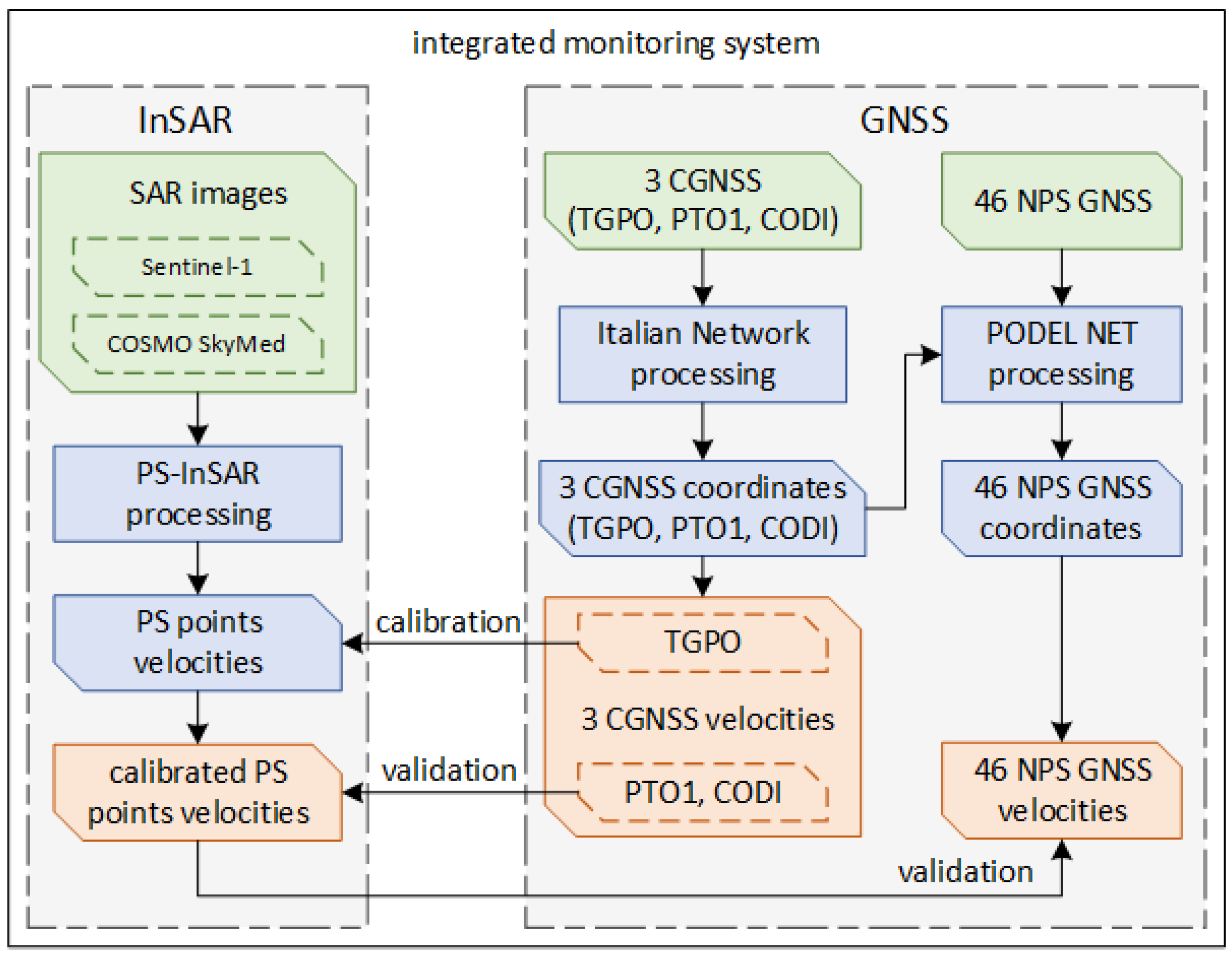
Figure 3.
Spatial and temporal distribution of CSK in the east (a) and west (b) stacks, and Sentinel-1 (c): the pentagrams representing the primary images and other symbols indicating the secondary images. (d) Temporal distribution of non-permanent GNSS. CGNSS data of TGPO, PTO1, and CODI stations were available continuously in the analyzed period.
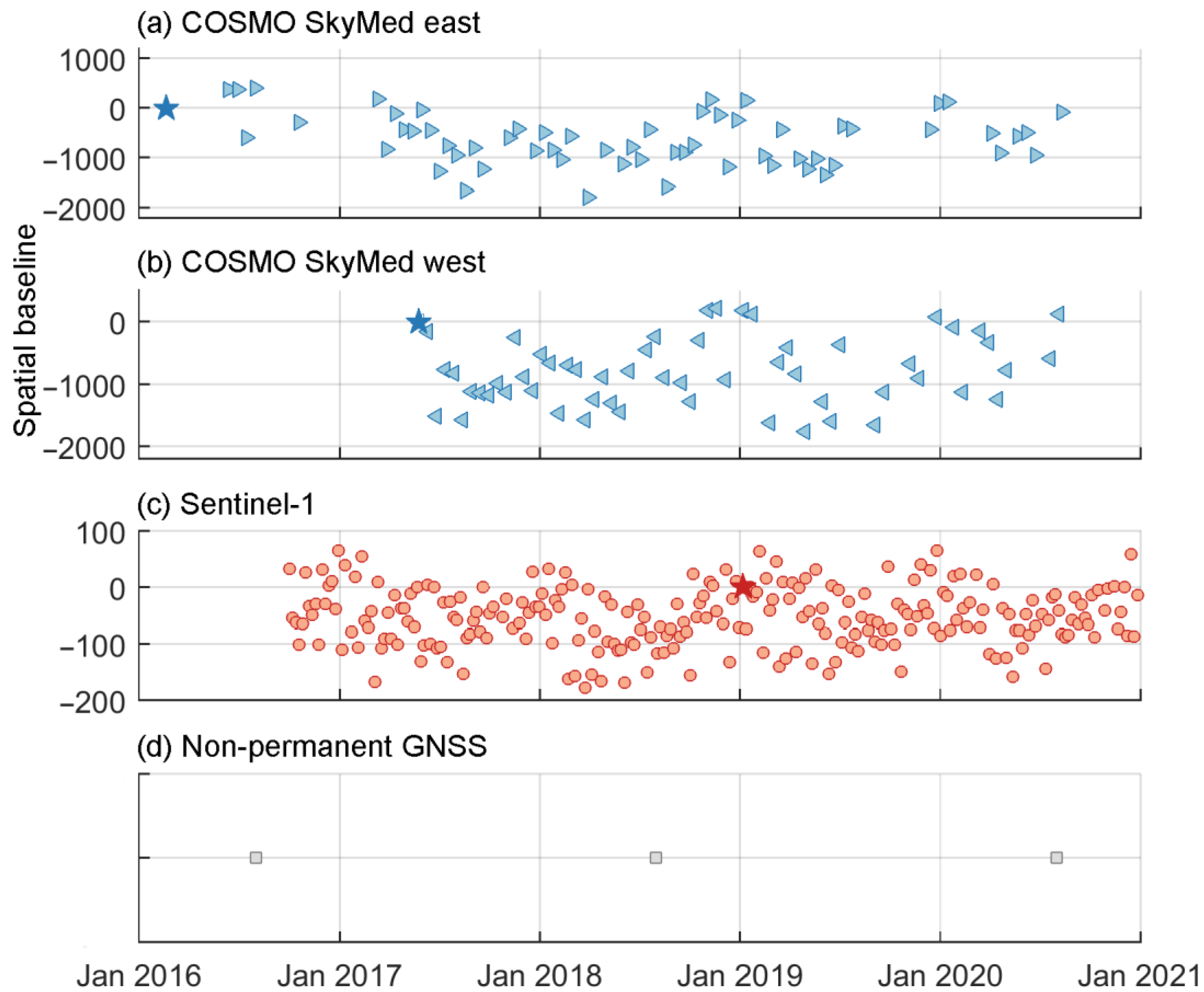
Figure 4.
Examples of NPS sites of the PODELNET network located in urbanized (a,b) and vegetated (c,d) areas.
Figure 4.
Examples of NPS sites of the PODELNET network located in urbanized (a,b) and vegetated (c,d) areas.

Figure 5.
Vertical velocities of the PODELNET GNSS network obtained from the surveys performed in 2016, 2018, and 2020.
Figure 5.
Vertical velocities of the PODELNET GNSS network obtained from the surveys performed in 2016, 2018, and 2020.
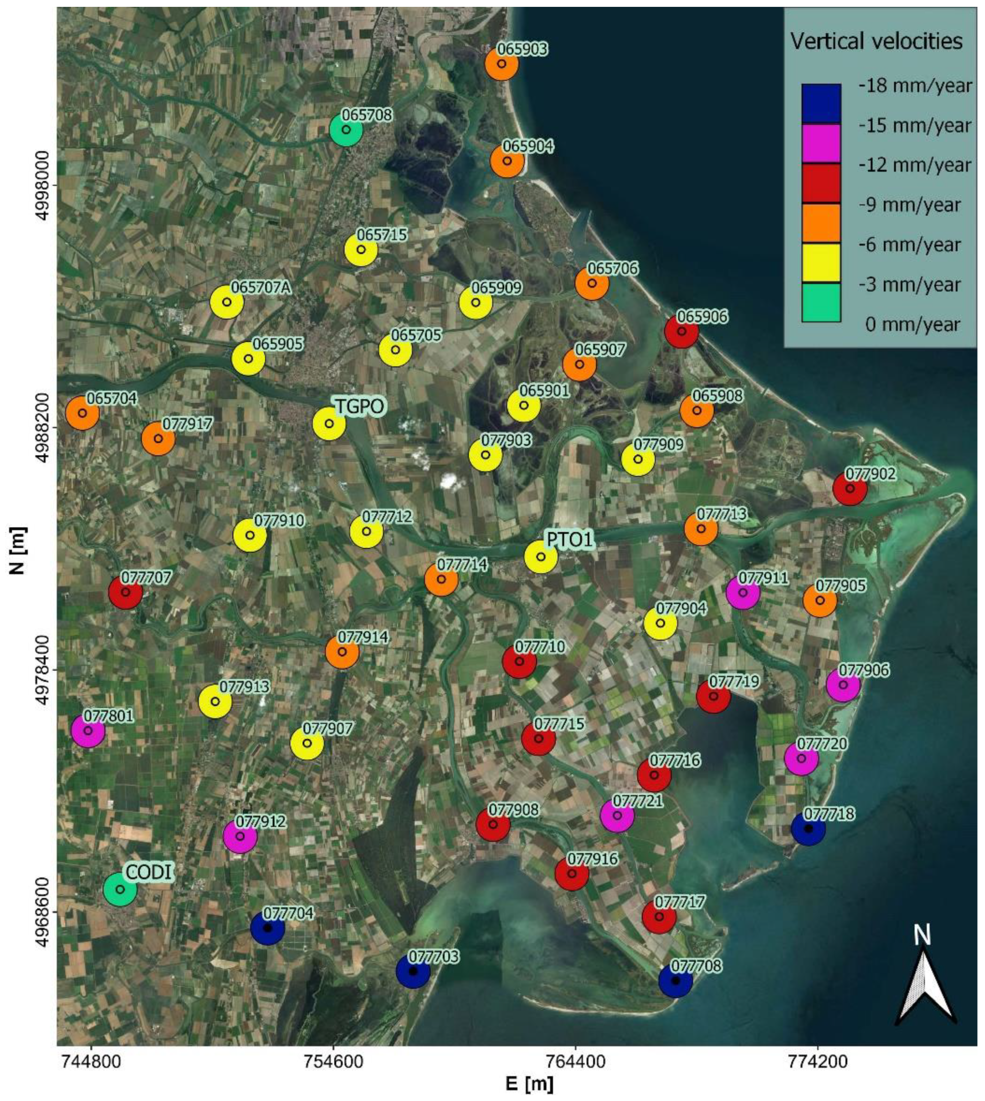
Figure 6.
Classification of the GNSS and InSAR points based on the LOS velocities considering six classes from 0 mm/year to −18 mm/year: (a) GNSS and Sentinel-1 points; (b) GNSS and CSK points.
Figure 6.
Classification of the GNSS and InSAR points based on the LOS velocities considering six classes from 0 mm/year to −18 mm/year: (a) GNSS and Sentinel-1 points; (b) GNSS and CSK points.
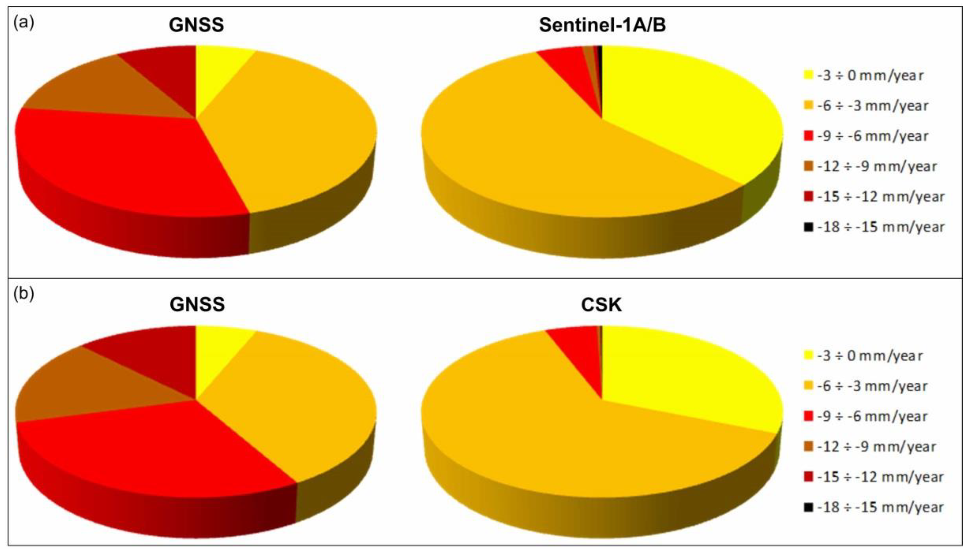
Figure 7.
Comparison between the LOS displacements time series of three NPS GNSS sites characterized by different velocities (065708, 077904, and 077902, Figure 1, Table 3) and the closest Sentinel-1 (left) and the CSK (right) points.
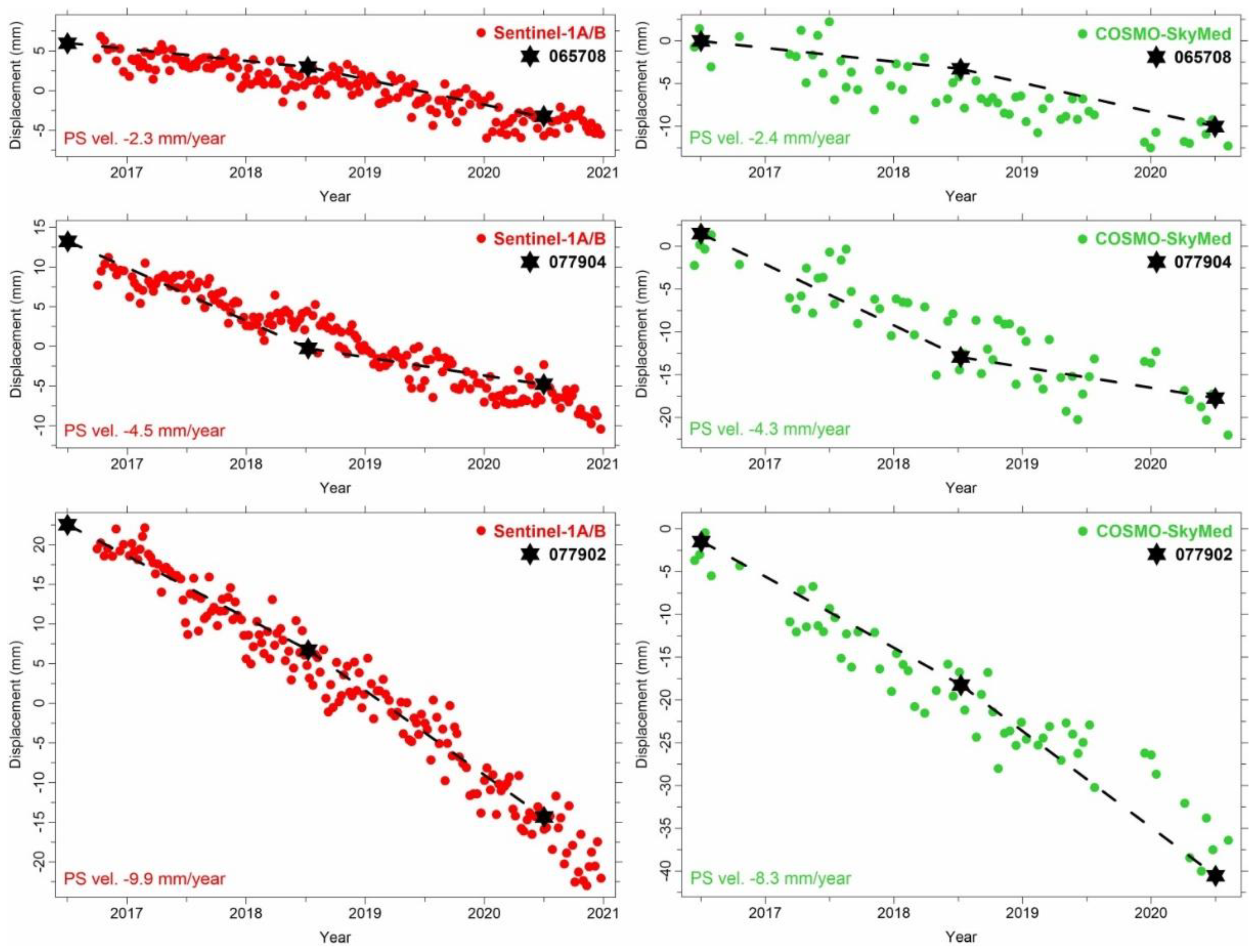
Figure 8.
Kinematic pattern of the LOS velocities in the study area: (a) GNSS and Sentinel-1 points; (b) GNSS and CSK points. The A, B, and C areas are shown in detail in Figure 9.
Figure 8.
Kinematic pattern of the LOS velocities in the study area: (a) GNSS and Sentinel-1 points; (b) GNSS and CSK points. The A, B, and C areas are shown in detail in Figure 9.
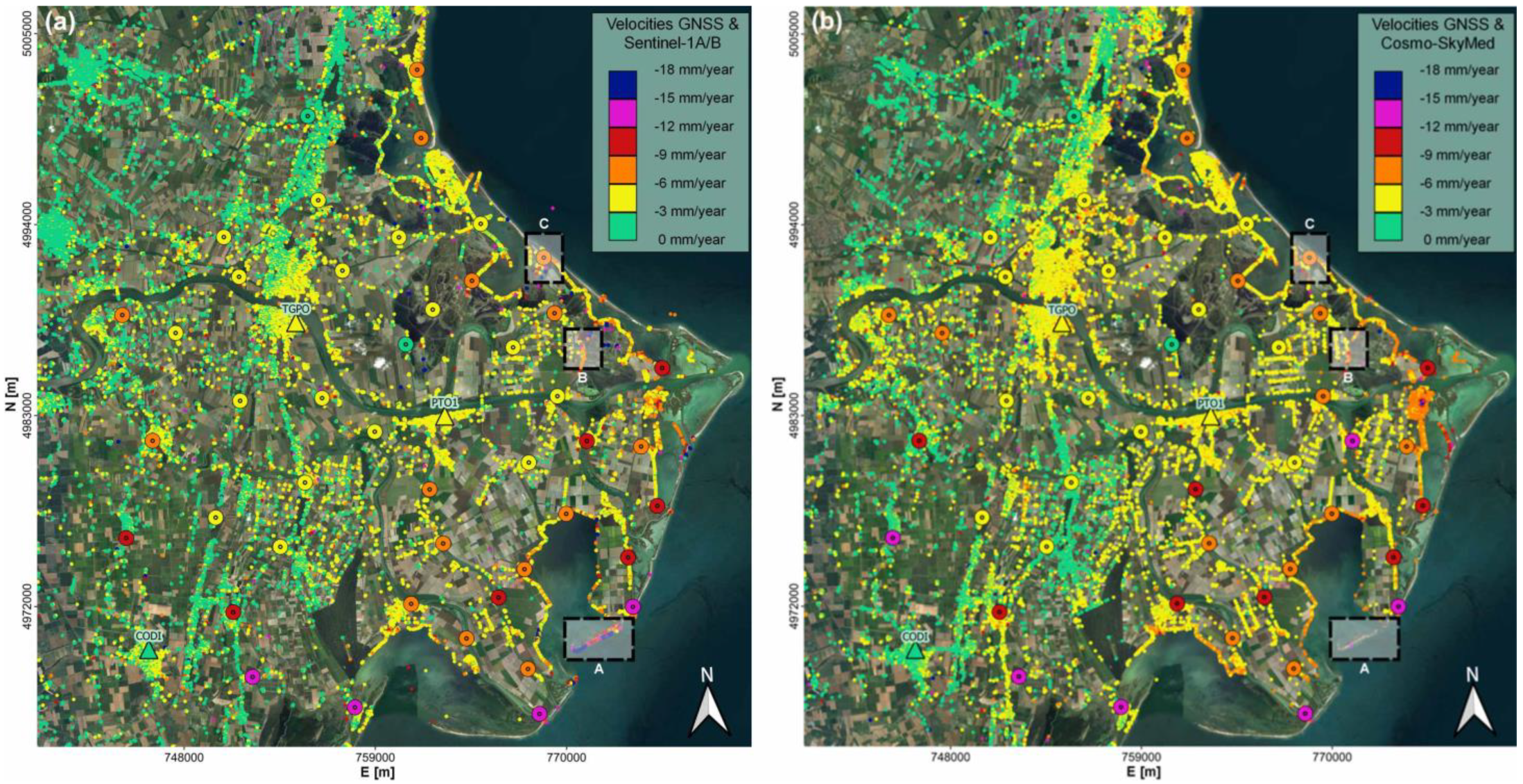
Figure 9.
Comparison between Sentinel-1 and CSK PS data. Due to the high subsidence rates caused by marine erosion (a,b), and/or documented anthropogenic activities on levees (reinforcement works) (c–f), Sentinel-1 data showed a better performance.
Figure 9.
Comparison between Sentinel-1 and CSK PS data. Due to the high subsidence rates caused by marine erosion (a,b), and/or documented anthropogenic activities on levees (reinforcement works) (c–f), Sentinel-1 data showed a better performance.
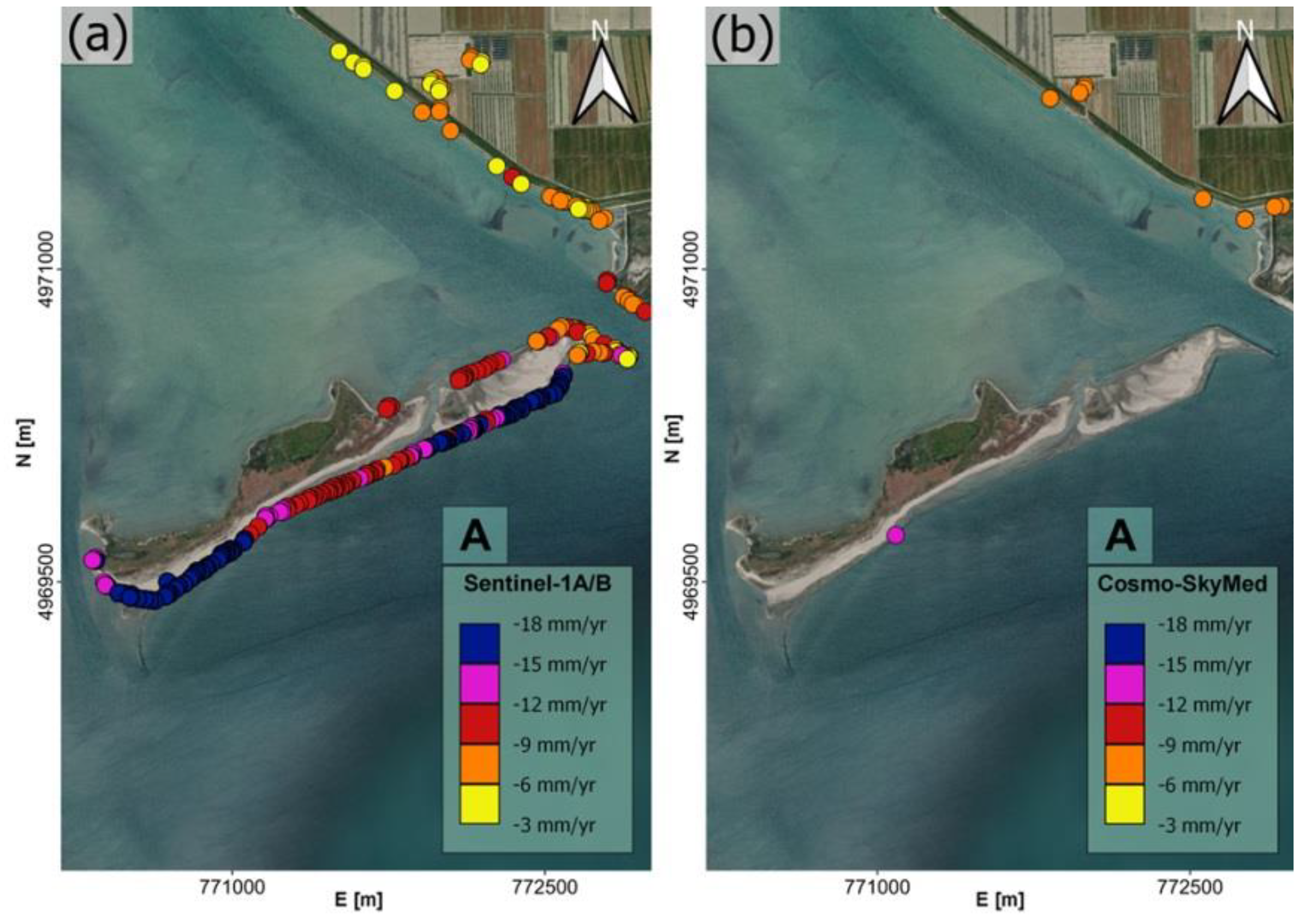
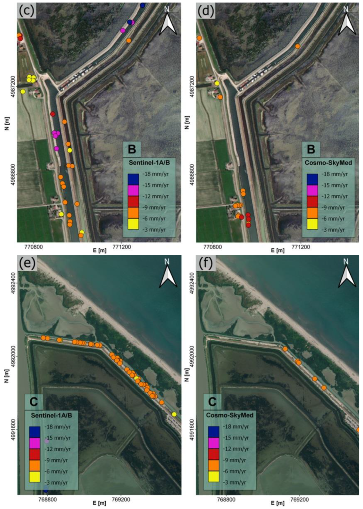
Figure 10.
Distribution of the LOS velocities in the study area overlapped to the highstand PRD lobe map (modified from [55]). For each sector enclosed by the polylines that highlight the expansion of the PRD over time, the LOS velocities and the related standard deviations were obtained by averaging the values of the available points. (a) GNSS and Sentinel-1 points; (b) GNSS and CSK points.

Figure 11.
Interpolation of the available GNSS-Sentinel-1 (a) and GNSS-CSK (b) data over the study area using the Kriging method with a grid size of 150 m (regional scale).
Figure 11.
Interpolation of the available GNSS-Sentinel-1 (a) and GNSS-CSK (b) data over the study area using the Kriging method with a grid size of 150 m (regional scale).


Table 1.
Vertical velocities of the 3 CGNSS stations estimated by [53] and during the present work (see text for more details).
Table 1.
Vertical velocities of the 3 CGNSS stations estimated by [53] and during the present work (see text for more details).
| Code | * Vv (mm/Year) (Period) | * Vv (2016–2018) (mm/Year) | ** Vv (2016–2018) (mm/Year) | ** Vv (2016–2020) (mm/Year) |
|---|---|---|---|---|
| CODI | −3.5 ± 0.7 (2007–2019) | −3.1 ± 0.4 | −2.8 ± 1.7 | −2.8 ± 1.8 |
| PTO1 | −5.8 ± 1.0 (2010–2019) | −5.8 ± 0.4 | −5.1 ± 2.2 | −5.1 ± 2.0 |
| TGPO | −5.6 ± 0.8 (2008–2019) | −6.5 ± 0.4 | −5.0 ± 1.8 | −5.1 ± 1.9 |
* [53]. ** This work.
Table 2.
Comparison between the vertical velocities of CODI, PTO1, and TGPO CGNSS measurements projected along the LOS of the satellites and PS points located up to 200 m from the permanent stations. In the case of CSK, the velocities before and after calibration are reported (see text for more details).
| CGNSS Station Code | Distance from the Station (m) | Sentinel-1 | COSMO-SkyMed | |||||
|---|---|---|---|---|---|---|---|---|
| N. of PS | PS Vel. (mm/Year) | CGNSS Vel. (mm/Year) | N. of PS | * PS Vel. (mm/Year) | ** PS Vel. (mm/Year) | CGNSS Vel. (mm/Year) | ||
| CODI | - | 1 | −2.7 | −2.2 ± 0.4 | 1 | −5.0 | −3.0 | −2.5 ± 0.4 |
| - | 2 | −2.6 ± 0.1 | 2 | −4.7 ± 0.3 | −2.7 ± 0.3 | |||
| - | 3 | −2.7 ± 0.2 | 3 | −4.7 ± 0.2 | −2.7 ± 0.2 | |||
| 50 | 4 | −2.7 ± 0.2 | 6 | −4.4 ± 1.1 | −2.4 ± 1.1 | |||
| 100 | 32 | −3.0 ± 0.4 | 44 | −4.5 ± 0.5 | −2.5 ± 0.5 | |||
| 150 | 55 | −3.1 ± 0.4 | 92 | −4.6 ± 0.7 | −2.6 ± 0.7 | |||
| 200 | 71 | −3.2 ± 0.5 | 147 | −4.6 ± 0.7 | −2.6 ± 0.7 | |||
| PTO1 | - | 1 | −4.5 | −4.0 ± 0.5 | 1 | −6.8 | −4.8 | −4.2 ± 0.5 |
| - | 2 | −4.5 ± 0.0 | 2 | −7.3 ± 0.6 | −5.3 ± 0.6 | |||
| - | 3 | −4.5 ± 0.0 | 3 | −7.3 ± 0.5 | −5.3 ± 0.5 | |||
| 50 | 10 | −4.5 ± 0.3 | 31 | −6.9 ± 0.4 | −4.9 ± 0.4 | |||
| 100 | 38 | −4.5 ± 0.3 | 171 | −7.2 ± 0.5 | −5.2 ± 0.5 | |||
| 150 | 62 | −4.4 ± 0.9 | 315 | −7.2 ± 0.5 | −5.2 ± 0.5 | |||
| 200 | 102 | −4.4 ± 0.8 | 461 | −7.2 ± 0.8 | −5.2 ± 0.8 | |||
| TGPO | - | 1 | −4.1 | −4.0 ± 0.5 | 1 | −6.4 | −4.4 | −4.2 ± 0.5 |
| - | 2 | −3.9 ± 0.1 | 2 | −6.5 ± 0.0 | −4.5 ± 0.0 | |||
| - | 3 | −4.0 ± 0.1 | 3 | −6.6 ± 0.2 | −4.6 ± 0.2 | |||
| 50 | 3 | −3.9 ± 0.1 | 16 | −6.4 ± 0.4 | −4.4 ± 0.4 | |||
| 100 | 21 | −3.9 ± 0.4 | 75 | −6.2 ± 0.6 | −4.2 ± 0.6 | |||
| 150 | 42 | −4.0 ± 0.3 | 128 | −6.2 ± 0.6 | −4.2 ± 0.6 | |||
| 200 | 60 | −4.1 ± 1.2 | 199 | −6.2 ± 0.6 | −4.2 ± 0.6 | |||
* Before calibration. ** after calibration.
Table 3.
Comparison between the LOS velocities of the PODELNET sites and the mean velocities of PS points within a circle centered on the NPS and with a radius of 200 m.
Table 3.
Comparison between the LOS velocities of the PODELNET sites and the mean velocities of PS points within a circle centered on the NPS and with a radius of 200 m.
| NPS Code | Sentinel-1 | COSMO-SkyMed | ||||||
|---|---|---|---|---|---|---|---|---|
| GNSS Velocity (mm/Year) | Number of PS | PS Velocity (mm/Year) | Difference (mm/Year) | GNSS Velocity (mm/Year) | Number of PS | PS Velocity (mm/Year) | Difference (mm/Year) | |
| 065704 | −6.8 | 3 | −3.2 ± 0.1 | −3.6 | −7.9 | 3 | −3.1 ± 0.4 | −4.8 |
| 065705 | −3.9 | 5 | −3.3 ± 0.1 | −0.6 | −4.2 | 6 | −3.5 ± 0.5 | −0.7 |
| 065706 | −5.3 | 49 | −4.1 ± 0.9 | −1.2 | −5.7 | 139 | −5.5 ± 1.6 | −0.2 |
| 065707A | −3.6 | 26 | −3.8 ± 1.6 | 0.2 | −4.2 | 28 | −3.2 ± 1.5 | −1.0 |
| 065708 | −2.3 | 29 | −3.3 ± 1.9 | 1.0 | −2.5 | 166 | −3.2 ± 1.0 | 0.7 |
| 065715 | −3.2 | 18 | −2.7 ± 0.4 | −0.5 | −3.4 | 22 | −3.2 ± 0.6 | −0.2 |
| 065901 | −4.4 | 11 | −5.3 ± 1.4 | 0.9 | −4.7 | 19 | −4.8 ± 1.1 | 0.1 |
| 065903 | −6.8 | 39 | −5.6 ± 1.1 | −1.2 | −7.2 | 172 | −5.7 ± 1.0 | −1.5 |
| 065904 | −6.3 | 3 | −3.2 ± 0.3 | −3.1 | −6.8 | 8 | −3.3 ± 0.2 | −3.5 |
| 065905 | −4.2 | 7 | −4.6 ± 0.8 | 0.4 | −4.8 | 18 | −4.6 ± 0.8 | 0.2 |
| 065906 | −8.3 | 4 | −6.1 ± 1.7 | −2.2 | −8.9 | - | - | - |
| 065907 | −6.4 | 34 | −4.2 ± 1.3 | −2.2 | −6.9 | 65 | −5.3 ± 0.8 | −1.6 |
| 065908 | −6.4 | 10 | −4.8 ± 0.8 | −1.6 | −6.9 | 17 | −4.9 ± 1.4 | −2.0 |
| 065909 | −3.1 | 3 | −1.3 ± 1.3 | −1.8 | −3.3 | 59 | −3.5 ± 0.5 | 0.2 |
| 077703 | −12.6 | 20 | −3.9 ± 1.3 | −8.7 | −13.4 | 161 | −3.8 ± 0.7 | −9.6 |
| 077704 | −12.3 | 2 | −4.7 ± 0.3 | −7.6 | −13.2 | - | - | - |
| 077707 | −7.8 | 60 | −3.1 ± 0.6 | −4.7 | −9.0 | 125 | −2.6 ± 0.6 | −6.4 |
| 077708 | −13.4 | - | - | - | −14.3 | - | - | - |
| 077710 | −8.5 | 3 | −3.9 ± 1.0 | −4.6 | −9.1 | 8 | −4.8 ± 0.3 | −4.3 |
| 077712 | −3.5 | 17 | −3.3 ± 0.6 | −0.2 | −3.7 | 72 | −3.3 ± 0.9 | −0.4 |
| 077713 | −5.6 | - | - | - | −6.0 | - | - | - |
| 077714 | −5.2 | 11 | −3.4 ± 0.2 | −1.8 | −5.6 | 39 | −4.2 ± 0.4 | −1.4 |
| 077715 | −7.2 | - | - | - | −7.6 | - | - | - |
| 077716 | −7.5 | 12 | −4.9 ± 1.2 | −2.6 | −8.0 | 27 | −5.1 ± 1.5 | −2.9 |
| 077717 | −7.2 | 5 | −4.3 ± 0.5 | −2.9 | −7.7 | 8 | −5.1 ± 0.7 | −2.6 |
| 077718 | −11.6 | 8 | −6.7 ± 2.7 | −4.9 | −12.9 | 1 | −6.7 ± 0.0 | −6.2 |
| 077719 | −8.1 | 15 | −4.5 ± 0.7 | −3.6 | −8.6 | 33 | −5.7 ± 0.7 | −2.9 |
| 077720 | −9.2 | 7 | −4.3 ± 1.0 | −4.9 | −10.1 | 24 | −5.8 ± 0.7 | −4.3 |
| 077721 | −10.9 | 11 | −3.8 ± 0.3 | −7.1 | −11.6 | 21 | −4.6 ± 0.4 | −7.0 |
| 077801 | −11.4 | 36 | −2.7 ± 1.3 | −8.7 | −13.2 | 93 | −2.6 ± 0.9 | −10.6 |
| 077902 | −9.2 | 4 | −5.6 ± 2.5 | −3.6 | −9.8 | 2 | −8.4 ± 0.8 | −1.4 |
| 077903 | −2.7 | 11 | −3.6 ± 1.3 | 0.9 | −2.8 | 24 | −3.4 ± 0.6 | 0.6 |
| 077904 | −4.5 | 18 | −4.7 ± 1.8 | 0.2 | −4.8 | 61 | −4.6 ± 0.6 | −0.2 |
| 077905 | −6.2 | 8 | −5.5 ± 1.8 | −0.7 | −6.6 | 45 | −6.2 ± 1.9 | −0.4 |
| 077906 | −9.5 | 8 | −5.0 ± 0.6 | −4.5 | −10.2 | 9 | −5.2 ± 0.8 | −5.0 |
| 077907 | −3.6 | 30 | −2.4 ± 0.5 | −1.2 | −3.9 | 133 | −2.6 ± 0.5 | −1.3 |
| 077908 | −8.5 | 57 | −4.0 ± 1.0 | −4.5 | −9.1 | 378 | −4.2 ± 0.7 | −4.9 |
| 077909 | −3.7 | 2 | −4.2 ± 0.2 | 0.5 | −4.0 | 9 | −5.0 ± 1.3 | 1.0 |
| 077910 | −3.7 | 7 | −2.3 ± 0.8 | −1.4 | −4.2 | 7 | −2.1 ± 1.9 | −2.1 |
| 077911 | −11.5 | 23 | −3.4 ± 1.0 | −8.1 | −12.3 | 142 | −4.8 ± 0.8 | −7.5 |
| 077912 | −9.7 | 55 | −2.9 ± 1.6 | −6.8 | −10.4 | 188 | −1.9 ± 0.7 | −8.5 |
| 077913 | −3.4 | 2 | −1.9 ± 0.1 | −1.5 | −3.9 | 10 | −3.5 ± 1.1 | −0.4 |
| 077914 | −5.5 | 71 | −3.2 ± 0.8 | −2.3 | −5.9 | 319 | −4.5 ± 0.7 | −1.4 |
| 077916 | −7.9 | - | - | - | −8.4 | 4 | −6.9 ± 0.6 | −1.5 |
| 077917 | −5.6 | - | - | - | −6.5 | - | - | - |
| 065704 | −6.8 | 3 | −3.2 ± 0.1 | −3.6 | −7.9 | 3 | −3.1 ± 0.4 | −4.8 |
| 065705 | −3.9 | 5 | −3.3 ± 0.1 | −0.6 | −4.2 | 6 | −3.5 ± 0.5 | −0.7 |
Publisher’s Note: MDPI stays neutral with regard to jurisdictional claims in published maps and institutional affiliations. |
© 2022 by the authors. Licensee MDPI, Basel, Switzerland. This article is an open access article distributed under the terms and conditions of the Creative Commons Attribution (CC BY) license (https://creativecommons.org/licenses/by/4.0/).
Share and Cite
MDPI and ACS Style
Fabris, M.; Battaglia, M.; Chen, X.; Menin, A.; Monego, M.; Floris, M. An Integrated InSAR and GNSS Approach to Monitor Land Subsidence in the Po River Delta (Italy). Remote Sens. 2022, 14, 5578. https://doi.org/10.3390/rs14215578
AMA Style
Fabris M, Battaglia M, Chen X, Menin A, Monego M, Floris M. An Integrated InSAR and GNSS Approach to Monitor Land Subsidence in the Po River Delta (Italy). Remote Sensing. 2022; 14(21):5578. https://doi.org/10.3390/rs14215578
Chicago/Turabian StyleFabris, Massimo, Mattia Battaglia, Xue Chen, Andrea Menin, Michele Monego, and Mario Floris. 2022. "An Integrated InSAR and GNSS Approach to Monitor Land Subsidence in the Po River Delta (Italy)" Remote Sensing 14, no. 21: 5578. https://doi.org/10.3390/rs14215578
Note that from the first issue of 2016, this journal uses article numbers instead of page numbers. See further details here.