


Spatial Validation of Spectral Unmixing Results: A Case Study of Venice City


Research Institute for Geo-Hydrological Protection (IRPI), National Research Council (CNR), 06128 Perugia, Italy
Remote Sens. 2022, 14(20), 5165; https://doi.org/10.3390/rs14205165
Submission received: 8 September 2022
/
Revised: 4 October 2022
/
Accepted: 11 October 2022
/
Published: 15 October 2022
(This article belongs to the Special Issue Optical Remote Sensing Applications in Urban Areas II)
Abstract
:Since remote sensing images offer unique access to the distribution of land cover on earth, many countries are investing in this technique to monitor urban sprawl. For this purpose, the most widely used methodology is spectral unmixing which, after identifying the spectra of the mixed-pixel constituents, determines their fractional abundances in the pixel. However, the literature highlights shortcomings in spatial validation due to the lack of detailed ground truth knowledge and proposes five key requirements for accurate reference fractional abundance maps: they should cover most of the area, their spatial resolution should be higher than that of the results, they should be validated using other ground truth data, the full range of abundances should be validated, and errors in co-localization and spatial resampling should be minimized. However, most proposed reference maps met two or three requirements and none met all five. In situ and remote data acquired in Venice were exploited to meet all five requirements. Moreover, to obtain more information about the validation procedure, not only reference spectra, synthetic image, and fractional abundance models (FAMs) that met all the requirements, but also other data, that no previous work exploited, were employed: reference fractional abundance maps that met four out of five requirements, and fractional abundance maps retrieved from the synthetic image. Briefly summarizing the main results obtained from MIVIS data, the average of spectral accuracies in root mean square error was equal to 0.025; using FAMs, the average of spatial accuracies in mean absolute error (MAEk-Totals) was equal to 1.32 and more than 78% of these values were related to sensor characteristics; using reference fractional abundance maps, the average MAEk-Totals value increased to 1.97 because errors in co-localization and spatial-resampling affected about 29% of these values. In conclusion, meeting all requirements and the exploitation of different reference data increase the spatial accuracy, upgrade the validation procedure, and improve the knowledge of accuracy.
1. Introduction
The spatial resolution (i.e., the ability to resolve two adjacent points as separate in the image) is one of the features of remote sensing imaging systems [1]. Some researchers highlight that, no matter how high the spatial resolution might be, the instantaneous field of view of image sensors always includes several discrete elements and no image pixel is completely homogeneous in spectral characteristics [2,3,4]. Therefore, the spectrum of each pixel is caused by a mixture of spectral signals (mixed pixels) and image processing techniques that are based on spatial analysis are not applicable [2,3,4,5]. In any case, since 1979, there has been a combined research effort to retrieve mixed pixel information from remote sensing images [6]. This effort has made possible the development of a systematic methodology that was given several slightly different names: linear mixing, spectral mixing models, spectral mixture analysis, spectral mixture modeling, and spectral unmixing [7,8,9,10,11,12]. In this paper, the term spectral unmixing was chosen from these. This methodology can be decomposed in two consecutive procedures: the first compares the spectrum of each mixed pixel with reference spectra to decompose it into a collection of constituent spectra (called endmembers); the second determines the proportion of each endmember present in the pixel (called fractional abundance) [4,12,13]. Since the number of endmembers must be less than the number of bands [7], some authors associated the development and use of spectral unmixing only with hyperspectral data [3,12,13,14]. However, the literature shows that, for over 40 years, spectral unmixing has been the most commonly used procedure for analyzing not only hyperspectral, but also multispectral images (e.g., [15]). Additionally, it is used for more and more applications from monitoring terrestrial environments (e.g., [16]) to extraterrestrial ones (e.g., [7]). One among these applications is urban land cover mapping which is now, more than ever, essential to understanding the impact of growing urban areas on the environment [12,17,18,19,20]. Spectral unmixing was exploited to distinguish urban surface materials from each other and from the background using hyperspectral (e.g., [21]) and multispectral (e.g., [22]) images at high spatial resolution and using hyperspectral (e.g., [18]) and multispectral (e.g., [23]) images at moderate spatial resolution, whereas it was exploited to distinguish urban area from the background using multispectral images at coarse spatial resolution (e.g., [20]).
To separate mixed pixel spectra into a collection of endmembers (i.e., the first procedure of spectral unmixing), the literature highlights two main models: linear (LMM) and nonlinear mixture models (NLMM). They assume two different behaviors of radiation reflected from each constituent material of the mixed pixel [4,12,24]. The light is completely separated before being mixed within the sensor in LMM’s case, whereas it is multiply scattered in NLMM’s case [4]. The choice between LMM or NLMM is still disputed; some authors pointed out that it might depend on the scale of the endmembers and the accuracy of the fractional abundance required [4]. However, LMM was the most widely employed in many scenarios [4,24], whereas NLMM was mainly applied to retrieve fractional abundance of minerals in soils [4]. To solve the inverse method which estimates the fractional abundances of each endmember (i.e., the second procedure), many solutions were proposed (e.g., Gram–Schmidt orthogonalization [25], least square methods [26], minimum variance methods [4], singular value decomposition [27], and variable endmember methods [4]). The least squares methods employed in LMM are the most utilized approaches because they provide an acceptable approximation of the light scattering mechanisms by minimizing errors [4,12].
Since 1986, many spectral unmixing techniques have been introduced to upgrade the mathematical validity of the model (e.g., [14,28]), but spatial and spectral validation of the results with ground truth data is still difficult to achieve (e.g., [4,24]). The spectral accuracy of spectral unmixing results can be evaluated using spectral signatures that were acquired in situ and/or in the laboratory and/or obtained from images. The previous works employed the spectra as reference spectral library to determine the endmembers present in the pixel and validate the results measuring their spectral accuracy (e.g., [14,20]). The flowchart of this spectral validation method is shown in Figure 1a. In the flowchart, reference data utilized as input into a process is connected to it by a red arrow, whereas reference data used for the validation process are connected to it by a green arrow (Figure 1a). The selection of an accurate and complete reference spectral library is essential because the key to spectral unmixing is the determination of endmembers [4,24,29,30]. Some authors created a synthetic image exploiting these spectra and the reference map in order to test the proposed procedure and/or to validate endmember extraction [14,31,32,33] and/or fractional abundance estimation (Figure 1b) [31,32,34,35]. Among these authors, only Dobigeon et al. [32] and Jia and Qian [31] exploited synthetic images to validate spectral unmixing results both spectrally and spatially.
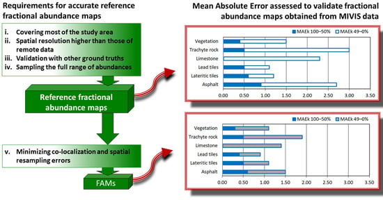
The lack of detailed knowledge of the ground truth was identified as the main reason for the many shortcomings in spatial validation of spectral unmixing results [4,18,24]. The authors detected and addressed five requirements for an accurate reference map: (i) these data should cover most of the study area rather than just a few pixels to characterize the overall accuracy of the results [6]; (ii) the spatial resolutions of these maps should be higher than those of fractional abundance maps that need to be validated [18,36,37]; (iii) these maps should be validated using other ground truth data to properly become ground truth data [36,38,39]. Because no map can fully and completely map the ground truth (i.e., territory [40]), it is more correct to call them reference maps than ground truth maps [41]; (iv) these maps should include accurate detail of fractional abundances to validate the full range of their values that were obtained by spectral unmixing [12,33,37,39]; (v) these data should minimize errors in co-localization and spatial resampling due to the comparison of different data at different spatial resolutions (i.e., remote data and reference maps) in the spatial validation procedures [33,42]. In Figure 2, the flowchart of the spatial validation model highlights the five requirements identified for accurate reference maps, highlighting that previous papers did not meet all requirements at the same time, but most papers met two or three requirements.
The first and second requirements were shared by most authors. Some created reference maps of the study area by exploiting high spatial resolution aerial imagery in order to validate spectral unmixing results that were obtained from coarse spatial resolution imagery (e.g., [18,37]). Dobigeon et al. [32] extracted information of the ground cover fraction distributions from digital photographs. Other authors exploited the data that were acquired during the field surveys in order to photo-interpret IKONOS image [23,33] or aerial photos [43] and created reference maps of the study area. In order to validate the fractional abundances obtained from MODIS images, Kim et al. [44] utilized a Landsat image classified with three different approaches. Kruse [45] performed the same procedures on AVIRIS (at spatial resolution equal to 20 m) and Hyperion (at spatial resolution equal to 30 m) images and exploited the results of the first data to evaluate the accuracy of the second. In order to validate the fractional abundances obtained from NOAA-AVHRR data, Puyou-Lascassies et al. [46] utilized SPOT-HRV images classified and aerial photographs. Williams et al. [36,39] spatially resampled a NEON D17 image at 0.25 m to validate the fractional abundances obtained from AVIRIS imagery. It is interesting to note that most of these reference maps represent urban contexts [18,23,31,33,37,38].
The third requirement was only met by Walton [38] and Williams et al. [36,39] which validated the reference map using airborne images and associated the error with it. The four requirements were met by few authors [12,33,37,39]. The reference fractional abundance maps ranking from 100 to 0% were produced by [12,33,37,39] in order to compare the results of the spectral unmixing proposed and by [43] in order to validate the results of three machine learning regression techniques. However, the authors started from knowledge of only a few abundance values and interpolated the rest of the range (e.g., [33]). The fifth requirement was only fulfilled by Cavalli [33] who compared the histograms of fractional abundance that were obtained from reference maps (FAMs) and fractional abundance maps. Table 1 summarizes the requirements and the authors that proposed and met them. In conclusion, most papers met two or three requirements of the reference maps and not all five (Figure 2).
Therefore, this work created reference fractional abundance maps, meeting all requirements, in order to analyze their advantages in improving the spatial validation of spectral unmixing results. Moreover, in order to gain more information about result accuracy, it employed not only FAMs that met five out of five requirements, but also other data: reference spectra, reference fractional abundance maps that meet four out of five requirements, synthetic images, and fractional abundance maps retrieved from synthetic images. Therefore, this paper not only fulfilled all the requirements for an accurate reference map that no other previous paper satisfied, but also, it utilized other data that no previous work exploited: reference fractional abundance maps that meet four out of five requirements, and fractional abundance maps retrieved from synthetic images. For this purpose, ground truth data of the historical center of Venice and a MIVIS image which was acquired simultaneously with an in situ campaign were exploited [47]. The results of this work emphasize that reference maps that meet all requirements and their integrated use with different types of reference data increase the spatial accuracy, improve the knowledge of accuracies, and upgrade the validation procedure.
2. Materials and Methods
2.1. Reference Map and Reference Spectra
2.1.1. In Situ and Remote Data
An urban area was chosen as the study area for two reasons: firstly, the spectral unmixing is the methodology most often employed to map urban cover materials (e.g., [20]); secondly, the urban pattern facilitates the creation of fractional reference abundance maps (e.g., [37]). Among many urban areas, the historical center of Venice was preferred because several field campaigns were carried out to spatially and spectrally characterize urban surface materials [23,47]. On 26 July 2001 at 10:45 a.m. (GMT), in conjunction with an in situ campaign, MIVIS (Multispectral Infrared and Visible Imaging Spectrometer) airborne data were acquired with a scan rate of 25 scans/sec at an altitude of 4000 m, corresponding to a ground resolution of 8 m (Table 2).
Moreover, in a previous work, different classifiers that were also applied to these remote data and a reference map that met only the first two requirements was utilized to validate their results [23]. Their comparison pointed out that the most consistent results were obtained from the spectral unmixing followed by the results obtained from a spectral angle mapper (SAM) supervised classification algorithm [23].
The city of Venice, known worldwide, is located inside a large lagoon in the northwestern Adriatic Sea which is named after the city (Figure 3a). One hundred and eighteen small islands, on which Venice is built, and three hundred and fifty-five bridges, that connect them together, are two of the special characteristics of Venice (Figure 3b). A bridge also connects the mainland to the western part of the city, which is the only portion accessible by wheeled vehicles. In the rest of the city, the movement of people and things is by pedestrian way or by boats. In the islands, the buildings arise close to one another and are separated by narrow streets (called “calli”), squares with different shapes (called “campi”), streams, and canals.
2.1.2. Reference Map Meeting All Requirements
In order to validate the fractional abundance maps retrieved from the MIVIS image, the reference map of Venice’s historical center, previously created by photo-interpreting a panchromatic IKONOS image [23,33], was exploited (i.e., the first and second requirements of reference maps, e.g., [36]). In order to meet the third requirement (e.g., [38]), this reference map was validated using other ground truth data. The city and lagoon portals of Venice supplied these additional ground truth data to validate it (i.e., the edges of pavement and canals, the ground limits of buildings and bridges, the map of houses of worship and public and private buildings, and limits and features of public green space [48,49]). These data were obtained integrating data that were derived from different methodologies (i.e., traditional topography, the GPS satellite system, and laser scanner [49]) and their characteristics of precision and spatial distribution generated ground truth maps at a spatial resolution of 0.02 m with a maximum error of 10%.
These data allowed us to validate four types of land covers: vegetation, pavement, and public and private roofs. Photointerpretation and knowledge of the area allowed us to differentiate between pavement materials and to eliminate all those areas whose cover material was uncertain. These steps led to the creation of six validated reference maps (Figure 4): (i) Asphalt, that paves the western part of the city and harbor areas; (ii) Lateritic tiles, that cover most buildings; (iii) Lead plates, that cover the public buildings and domes; (iv) Limestone, that came from the quarries of Pietra d’Istria (Italy), that decorates the pavement of the historical center, but only the decorations of the squares facing St. Mark’s Basilica and the train station were considered; (v) Trachyte rock, that came from quarries in the Euganean Hills (Italy), that paves pedestrian streets; (vi) Vegetation. Many uncertain areas were not included in the reference map to minimize the error as much as possible; however, it is impossible for the maps to totally match the ground truth [40].
In order to meet the fourth requirement (i.e., the characterization of the entire range of fractional abundances, e.g., [37]), the previous works started from the assumptions that when spatially resampling a mask, where all pixels are characterized by 100% abundance, at lower resolution, only some defined pixels will be characterized by 100% abundance; the abundances of the other pixels of the starting mask will decrease linearly with increasing distance from pixels having 100% abundance; and the distance between pixels with 100% abundance and those with 0% abundance will be equal to the spatial resolution of the remote image [12,33,37]. By knowing only a few abundance values, the previous papers interpolated the rest of the range, whereas the present work aims to best sample the entire range using more known values. For this purpose, the choice of spatial resolution of the starting reference maps was very important. The spatial resolution of 0.20 m was chosen to validate the results obtained from MIVIS image because the starting maps at this resolution allowed us to sample the range from 100 to 0% with 40 known values (i.e., 40 pixels with spatial resolution of 0.20 m is the same as 8 m). The ground truth data that were exploited to validate the previous reference map allowed us to achieve this spatial resolution [48,49]. Therefore, the reference map at spatial resolution of 0.20 m was divided into 6 masks corresponding to the 6 selected endmembers, and these data were used as input for the procedure of fractional abundance determining. Figure 5a shows a portion of previous reference map (white) [33] and validated reference map (green) of the trachyte endmember at the spatial resolution of 0.20 m. In Figure 3b, the area examined in Figure 5 is highlighted with a yellow square.
The proposed procedure, starting from the one previously presented, upgrades and complements it, since the previous procedure started from only three known values and interpolated the rest of the range considering a linear trend [33]. The new one involves two steps: the first step identifies the pixels that should have 100% abundance of each endmember. For this purpose, firstly, the starting reference maps were spatially resampled to the spatial resolution of the remote image by applying the nearest neighbor method; secondly, these resampled maps were spatially resampled to the resolution of the starting reference map by applying the bilinear convolution method; finally, the pixels remaining after the two spatial resamples were selected (red pixels in Figure 5b).
The literature highlights that nearest-neighbor resampling is the method most commonly employed in the ortho-rectification, resampling to a north–south grid process and aligning coarse-scale images on fine-scale ones (e.g., [50]). In any case, in order to identify the methods that best minimize error in spatial sampling, the results of the main image resampling methods (i.e., pixel aggregate, nearest neighbor, bilinear and cubic convolution methods) were compared (Figure 6 shows the same portion of the trachyte reference mask shown in Figure 5). In these figures, the starting mask (blue) is covered by a twice-resampled reference map which has two different colors: pixels are colored cyan when they fall within the boundaries of the source map, whereas they are colored red when they erroneously cross the boundaries of the source map. Figure 6a shows a smaller number of red pixels than the other figures, indicating that the application of nearest neighbor and bi-linear convolution methods, in this time order, minimizes errors due to image resampling.
The second step evaluates pixels that should have less than 100% abundance of the endmember. With regard to the portions of the mask surrounding the areas with 100% abundance, a set of areas equidistant from the 100% abundance pixels, within the higher resolution reference map, was created. A first area was created at a distance of one pixel, the second at a distance of two pixels, and so on until the distance was equal to the spatial resolution of the remote image (Figure 5c). These areas are associated with gradually decreasing abundance from 99 to 0%. With regard to the portions of the mask not surrounding the areas with 100% abundance, the directional filters at horizontal (0°) and vertical (90°) orientations were applied to this portion of the reference mask. A set of areas that were equidistant from the pixels identified with the filters was created within the higher-resolution reference map (Figure 5d). These areas are associated with gradually increasing abundance from 1 to 99%. In conclusion, all pixels associated with the 100 to 0% abundances of each endmember were identified and mapped to form the corresponding reference fractional abundance map (Figure 5d).
Lastly, to minimize co-localization and spatial resampling errors due to the comparison of different data (i.e., remote data and reference maps) at different spatial resolution (i.e., to meet the five requirements), the reference and retrieved fractional abundance maps were not compared, but the method proposed by Cavalli was exploited: the comparison of the abundance histograms of the reference fractional abundance maps and the fractional abundance maps obtained by spectral unmixing [33]. The histogram of reference fractional abundance maps was called the fractional abundance models (FAMs) [33].
2.1.3. Reference Spectra
Spectral characterization of the six identified materials was performed at several sites in the historical center to sample natural spectral variability and in the laboratory to better evaluate the spectral characteristics of the materials [23]. The field campaigns were conducted using a portable field spectrometer Analytical Spectral Devices FieldSpec Full-Range Pro [47]. The spectrometer sampled spectral range from 350 to 2500 nm using two detectors: one covered from 350 to 1050 nm with a spectral sampling interval of 1.4 nm, and the other covered from 1000 to 2500 nm with a spectral sampling interval of 2.0 nm. The field measurements were collected within 2 h of solar noon sets by acquiring 4–5 measures for each target from a height of 1 m using a field of view of 25° to fulfil the target dimension. A Spectralon reference standard (i.e., National Institute of Standards and Technology calibrated panel) was employed to derive absolute reflectance spectra [23,47]. Therefore, the created spectral library was spectral resampled according to the spectral characteristics of the MIVIS data to become the reference spectra.
2.2. Preprocessing and Spectral Unmixing Processing Chains
As regards radiometric calibration, MIVIS data were pre-processed employing an improved radiometric correction procedure [51]. Since the determination of the endmember was performed by exploiting reflectances that were acquired in situ and/or in the laboratory, radiance data were atmospherically corrected to obtain reflectance images. MIVIS radiance data were atmospherically corrected by means of the MODTRAN4 radiative transfer code [52,53]. Atmospheric correction data were validated using in situ spectral measurements [54]. After applying the spectral unmixing processing chain [55], the fractional abundance maps were geometrically corrected by exploiting an improved geometric correction procedure [56]. In order to compare the reference maps with the fractional abundance maps that were retrieved from MIVIS data, a set of ground control points (GCPs) was extracted from the IKONOS panchromatic image, and resampled to 0.20 m, to which the ground truth data used to validate the reference map [48,49] were superimposed. The MIVIS image yielded RMS errors of 0.064 pixels.
For most authors, the spectral unmixing processing chain applied to hyperspectral data includes not only endmember determination and inversion, but also dimension reduction (e.g., [12,13]). Therefore, minimum noise fraction (MNF) transformation [57] was applied to both datasets by using the forward MNF transform implemented in the ENVI 5.6 software package. In conclusion, MIVIS’s 92 bands were reduced to 47 bands.
Because multiple endmember spectral mixture analysis (MESMA) is the most widely used spectral unmixing methodology in the urban context (e.g., [17,18,37]), it was applied to the corrected MIVIS image exploiting an open-source software application ‘VIPER2-tools’ that is an ENVI add-on. MESMA, introduced by Roberts et al. [58], allows us to vary the number and types of endmembers for each pixel because spectral unmixing assumes that the set of endmembers present in a pixel is invariable. MESMA searches, among all possible combinations, the best combination of endmembers for each mixed pixel [58].
Since MESMA is based on LMM, mixed spectrum measured at pixel i can be denoted as a linear combination of endmember spectra:
where N is the number of the endmembers, fk is the fractional abundance of the endmember k, Sk is the spectrum of the endmember k, and ε is the residual error that takes into account the spectral and spatial characteristic of the sensor, noise and errors of the preprocessing and processing chains [4,12,13]. In the LMM, fractional abundances are subject to the following constraints:
2.3. Validation Methods of the Spectral Unmixing Results
The remote and in situ data of Venice historical center allowed us to spatially and spectrally validate the spectral unmixing results using five different reference data: reference spectra, synthetic image, reference fractional abundance maps that met four out of five requirements, fractional abundance maps retrieved from synthetic image, and FAMs that met all the requirements. A validation method was associated with each reference datum employed. Firstly, to validate the endmembers, the differences between the reference spectra and the spectra of the pixel constituents were measured for each pixel (called the first method, Figure 1a). This spectral validation method was employed by many authors (e.g., [20]). Secondly, to validate the endmembers, the similarity measures between the reference spectra and the pixel spectra of the real and synthetic image were compared (called the second method, Figure 7a). This spectral validation method was proposed by some authors (e.g., [31]); however, these authors created the synthetic images from reference maps that did not meet all the requirements (Figure 1b), whereas the reference fractional abundance maps that were employed to create the synthetic image met four out of five requirements (Figure 7a). Third, to validate the endmembers, the same spectral unmixing procedure was applied to both the true and synthetic images, and the differences between the reference spectra and the spectra of the pixel constituents, that were obtained from the true and synthetic images, were compared (called the third method, Figure 7b). Fourth, to spatially validate the results, the differences between the fractional abundance maps, that were obtained from the true and synthetic images, and the reference ones were calculated and compared (called the fourth method, Figure 7c). Lastly, to spatially validate the results, the differences between the fractional abundance maps, that were obtained from the true and synthetic images, and the FAMs were calculated and compared (called the fifth method, Figure 7d). In conclusion, the results of all these methods were compared. In the flowcharts of five validation methods shown in Figure 1a and Figure 7, the reference data are shown in green color and those utilized are highlighted with a yellow rectangle with a green border, whereas additional data utilized are highlighted with an orange rectangle.
Among these methods, four employ a synthetic image to spatially and spectrally validate the results (Figure 7a–d). In order to build the synthetic images, the six reference maps and spectral library were utilized and the procedure proposed by [33] was exploited in order to simulate the internal spectral variability of each endmember in the synthetic images. Each reference mask was multiplied by the corresponding endmember spectrum and its internal spectral variability [33] (i.e., imagining a chessboard of the same size and shape as the mask, its pixels that were associated with the black chessboard squares were multiplied by the mean spectrum plus the standard deviation, whereas those that were associated with the white chessboard squares were multiplied by the mean spectrum minus the standard deviation). The area previously mapped as a water body [33] was multiplied by the spectra of lagoon waters exploiting the same procedure again. In order to consider the spectral variability of all materials characterized in situ, the area remaining after removing the endmembers masks and that of the water body was multiplied by two average spectra utilizing the procedure proposed by [33]: imagining a checkerboard of the same size and shape as mask, one pixel as yes and one as no were multiplied by the average spectrum of the six identified endmembers plus the average spectrum of lagoon waters, and one pixel as no and one as yes were multiplied by the average spectrum of some ancillary materials (e.g., wood, cloth, plastic, and metal) plus the average spectrum of lagoon waters. Therefore, the starting hyperspectral image at a spatial resolution of 0.30 m with 47 bands was spatially resampled at 8 m to simulate the MIVIS image. This spatial resolution, different from that identified to create the reference maps and FAMs (i.e., 0.20 m), was chosen to maintain spectral variability in the synthetic image since the pixels at a resolution of 8 m did not contain an integer or an even number of pixels at a resolution of 0.30 m. Simulating the internal spectral variability of endmembers and preserving it during spatial resampling is important because in high-spatial-resolution images, spectral unmixing results are also driven by internal spectral variability [33].
Spectral and spatial accuracy were previously assessed not only using differences between the retrieved and reference data (i.e., bias [59], mean absolute error [19], mean of all [36], mean square error [32], Pearson correlation coefficient [15], reconstruction error [60], root mean square error [14], and systematic error [19]), but also using spectral similarity measures (i.e., Euclidean distance [31], maximum likelihood algorithm [36], spectral angular distance [14], and spectral information divergence [31]). Both approaches were also utilized in this work to spatially and spectrally validate the spectral unmixing results (Table 3).
Since the root mean square error (RMS) of the residual errors (e.g., [20]) and mean absolute error (MAE) (e.g., [19]) were the most commonly used, they were selected to validate the pixel constituent spectra and fractional abundance maps, respectively. The average value of the residual errors of all pixels i within endmember mask k (RMSk) was given as:
where ni is the number of pixels i within endmember mask k; RMSk values were calculated by applying “VIPER2-tools” which determines the best set of endmembers by minimizing the RMS value for each pixel.
The MAE calculated for all pixels within endmember mask k (MAEk) was given as:
where the Aclassified and Areference are fractional abundances of the same pixel that were retrieved from remote and reference data, respectively. MAEk was calculated in the range of abundances from 100 to 0% (MAEk-Totals), in the range from 100 to 50% (MAEk-100–50%), and in the range from 49 to 0% (MAEk-49–0%). This distinction of abundance range was performed since it divides pixels that are assigned to an endmember from those that are not assigned [61].
As regards the similarity measures performed for spectral validation, spectral angular distance (SAD) was chosen because it is the most widely employed (e.g., [14]). The average value of SAD calculated of all pixels i within endmember mask k (SADk) was given as [62]:
where nb is the number of the bands j, and Sk are spectra of the pixel and reference endmember. Therefore, the spectral similarity measurement is close to the value 0 when the pixel spectrum is spectrally similar to the reference spectra and it is close to the value 1 when the spectrum is not spectrally similar.
The metrics previously utilized to evaluate the similarity between the pixel spectrum and reference spectra (i.e., Euclidean distance [31], maximum likelihood algorithm [36], spectral angular distance [14], and spectral information divergence [31]) were also exploited by four supervised classifiers (i.e., minimum distance, maximum likelihood, spectral angular mapper, and spectral information divergence, respectively). Since every supervised classifier successfully uses a different algorithm to measure the similarity between the pixel spectrum and reference spectra, spectral similarity measurements achieved by the main supervised classifiers (i.e., binary encoding, minimum distance, maximum likelihood, spectral angular mapper, and spectral information divergence) were taken into consideration to better assess the spectral similarity [63]. Therefore, these supervised classifiers were applied to the input images utilizing the same reference spectra, that were exploited to determine the spectra of the pixel constituents; five different spectral similarity measurements within each endmember mask were evaluated and the average of their values were normalized. The normalized average of spectral similarity measures (aSSMn), that were calculated for all pixels within endmember mask k is expressed as
where nc is the number of the supervised classification C, SSMCi is spectral similarity measurement that was calculated at pixel i within endmember mask by the supervised classifier C, and SSMCmin_k and SSMCmax_k are the minimum and maximum values of the spectral similarity measurements that were calculated by the supervised classifier C within endmember mask k. Therefore, when the pixel spectrum is spectrally similar to the reference spectrum, the normalized average value of spectral similarity measurements is close to the value 1, and when the pixel spectrum is not spectrally similar, it is close to the value 0. In conclusion, for each endmember, mean and standard deviation of SADk and aSSMnk values, that were evaluated within the corresponding mask, were calculated (i.e., SADk, aSSMnk, σSADk, and σaSSMnk).
Since the reference fractional abundance maps created meet four out of five requirements and the FAMs derived from these maps meet all requirements, also FAMs were exploited to spatially validate the fractional abundance maps. Kling–Gupta efficiency (KGE) was exploited to evaluate similarity between the FAM and the histogram of retrieved fractional abundances to the same endmember within its mask. KGE is given as [64]:
where R is linear correlation between the FAMs and retrieved fractional abundance histogram relative to the same endmember, σ is their standard deviation, and µ is their mean values. The KGE value is used to calibrate and evaluate not only the hydrological models, but also the bio-optical models [65]. The literature grouped the KGE values into three classes: values equal to 1, positive and negative values that indicate equal, approximately similar, and non-comparable distributions, respectively [64,65].
3. Results
3.1. Fractional Abundance Models (FAMs)
As mentioned above, the reference fractional abundance maps at a spatial resolution of 0.20 m allowed us to retrieve FAMs at a spatial resolution of 8 m: starting from the reference fractional abundance maps at spatial resolutions of 0.20 m, the range of the FAMs from 100 to 0% at the spatial resolution of 8 m was sampled with 40 known values in order to validate the results obtained from the MIVIS data. Figure 8 compares the FAMs of each selected endmember.
The analysis of the FAMs highlights that urban surface materials of Venice historical center which are characterized by large and non-jagged shapes (i.e., asphalt, lateritic tiles, and lead plates) show an initial linear trend and then tend to be zero confirming the results as reported by [12,33,37], whereas the other surface materials which are characterized by small and jagged shapes show a non-linear trend (i.e., limestone, trachyte rock, and vegetation).
3.2. Methods for Spectral Validating the Pixel Constituent Spectra
As mentioned in the previous section, the endmembers (i.e., pixel constituent spectra) were spectrally validated by measuring the difference (i.e., error) and similarity between the reference spectra and the spectrum of each image pixel (Table 3), which was placed within the reference mask of the corresponding endmember. The errors were calculated using RMSk values (Equation (4)); the values obtained by applying the first and third methods (Figure 1a and Figure 7b) are shown in the first and second columns of Table 4, respectively. The absolute differences between the RMSk (ΔRMSk) values that were retrieved from the true and synthetic images are shown in the third column of Table 4.
Since the focus of spectral unmixing is the determination of endmembers (e.g., [13]), the residual error values (ε, Equation (1)) and, consequently, the RMSk value (Equation (4)) attest to the accuracy of its results. With reference to the previous works (e.g., [66]), an RMS value smaller than 0.045 attests to good accuracy in determining endmembers. The RMSk values obtained from the MIVIS image ranged from 0.029 to 0.020 and the values obtained from the synthetic image ranged from 0.026 to 0.011. Therefore, the RMSk values obtained attest to good accuracy of the spectral unmixing procedure performed since they are below the previously proposed threshold (Figure 9).
The absolute differences between the RMSk values obtained from true and synthetic images (ΔRMSk) range from 0.015 to 0.002. It is important to mention that the spectral and spatial characteristics of the synthetic image are the same as those of the remote image and the procedure used to make the synthetic image is the same spectral unmixing procedure as that applied to the remote image. In other words, each spectrum of the synthetic image is the weighted sum of the reference spectra of the endmembers, whose weights are determined by the reference fractional abundance maps. Therefore, because differences between the RMSk values obtained from the true and synthetic images are equal to about 30% of the RMSk value obtained from the true image, the remaining 70% can be attributed to the spectral and spatial characteristics of the MIVIS image and confirms the choice of not only the set of endmembers, but also the linear mixture model.
In detail, the choices of the reference endmember set and the LMM are more accurate for the endmembers of building roofing materials and vegetation (i.e., more than 91% of the RMSk values, Figure 10) than for the ones of street paving materials (i.e., less than 62% of the RMSk values, respectively, Figure 10), where the effect of multiple scattering and the occurrence of other surface materials (i.e., the surface of street paving materials was mapped as totally empty of people and things) may be slightly greater.
As regards similarity measures between the reference spectra and the spectrum of each image pixel placed within the corresponding reference mask, they were evaluated using the SADk and aSSMnk values (Equation (6) and Equation (7), respectively) and their standard deviation values. However, it is important to remember that, when the pixel spectrum is similar to the reference spectrum, the SAD value is close to 0 whereas the SSMn value is close to 1. Conversely, when the pixel spectrum is not similar to the reference spectrum, the value of SAD is close to 1, while the value of SSMn is close to 0. The SADk, σSADk, aSSMnk, and σaSSMnk values obtained from true and synthetic images are shown in the first and second four rows of Table 5, respectively. The absolute differences between the values that were retrieved from true and synthetic images are shown in the third four rows of Table 5.
The spectra of the MIVIS image within the reference masks are slightly less similar to the corresponding reference spectra than those of the synthetic image (i.e., the average values of SADi and aSSMnk obtained from the true image are equal to 0.345 and 0.595, respectively, and the average values of SADk and aSSMnk obtained from the synthetic image are equal to 0.279 and 0.681, respectively). In the true and synthetic images’ processing, the endmembers showing the greatest values were lead plates, lateritic tiles and vegetation, whereas the ones showing the smallest values were the endmembers of street paving materials. As regards true image processing, the standard deviation of the SADk and aSSMnk values calculated for endmembers of street paving materials (i.e., the average values of σSADk and σaSSMnk were equal to 0.132 and 0.514, respectively) were greater than the ones that were calculated for building roofing materials (i.e., the average values of σSADk and saSSMnk were equal to 0.077 and 0.251, respectively). Contrastingly, in the synthetic image processing, the standard deviation of the SADk and aSSMnk values calculated for endmembers of street paving materials (i.e., the average values of σSADk and σaSSMnk values were equal to 0.052 and 0.219, respectively) were quite similar to the ones that were calculated for building roofing materials (i.e., the average values of σSADk and σaSSMnk values were equal to 0.053 and 0.283, respectively). In conclusion, the pixels within the reference masks of the street paving materials are less similar to the corresponding reference spectra than those inside the reference masks of the building roofing materials. Therefore, the similarity measures also confirmed what was evidenced by the error measures: the effect of multiple scattering and the presence of other surface materials affect the pixels of street paving materials more than the pixels of building roofing materials.
3.3. Methods for Spatial Validating the Fractional Abundance Maps
The error and similarity measures were also evaluated to spatially validate the spectral unmixing results. In the fourth method (Figure 7c), the spatial accuracy of fractional abundance maps was evaluated by measuring the differences between the fractional abundance retrieved from true and synthetic images and the fractional abundance of the corresponding reference map that met four out of five requirements. For each endmember, only the errors of pixels placed within the corresponding reference mask were considered. The errors were calculated with MAEk-Totals, MAEk-100–50%, and MAEk-49–0% values (Equation (5)) and these values obtained from true and synthetic images are shown in Figure 11.
The MAEk-Totals values obtained from the processing of the MIVIS image using reference fractional abundance maps were less than 3.0 (Figure 11). In detail, the endmembers of trachyte rock and asphalt showed the greatest errors, followed by limestone and then vegetation; lastly, the endmembers of building roofing materials showed the smallest values. Moreover, MAEk-Totals values calculated from true images were about two times greater than ones calculated from synthetic images (i.e., the average value of MAEk-Totals obtained from the true image was equal to 1.97, whereas the average value of MAEk-Totals obtained from the synthetic image was equal to 0.99). Therefore, about 50% of MAEk-Totals was due to sensor characteristics, the reference endmember set and LMM (Figure 12). In detail, the choices of the reference endmember set and the LMM were more accurate for the endmembers of building roofing materials and vegetation (i.e., more than 68% of the MAEk-Totals values, Figure 12) than for ones of street paving materials (i.e., less than 48% of the MAEk-Totals values, Figure 12).
As regards MAEk-100–50% and MAEk-49–0% values calculated from the MIVIS image, the MAEk-49–0% values were about three times greater than the MAEk-100–50% values (i.e., the average value of MAEk-100–50% was equal to 0.48 whereas the average value of MAEk-49–0% was equal to 1.48, Figure 11). As regards MAEk-100–50% and MAEk-49–0% values calculated from the synthetic image, MAEk-49–0% values were about 2.5 times greater than MAEk-100–50% values (i.e., the average value of MAEk-100–50% obtained was equal to 0.29 whereas the average value of MAEk-49–0% was equal to 0.69, Figure 11). These values show that fractional abundances from 49 to 0% are overestimated by maps retrieved from true and synthetic images [33], and this overestimation is more in maps retrieved from true images than in maps retrieved from synthetic images.
The fifth method (Figure 7d) aims to minimize errors in co-localization and spatial resampling due to the comparison of different data at different spatial resolutions in the spatial validation procedures. Therefore, the histograms of fractional abundances retrieved from true and synthetic images were compared with the FAMs in order to evaluate spatial accuracy using error and similarity measurements. Error measures calculated from true and synthetic images were measured with MAEk-Totals, MAEk-100–50%, and MAEk-49–0% values and these values are shown in Figure 13.
In general, the MAEk-Totals values obtained from the MIVIS image using FAMs were less than 1.9, whereas the values obtained from the synthetic images were less than 1.4 (Figure 13). In detail, as regards true image processing, the endmember of trachyte rock showed the greatest values, followed by asphalt and limestone, respectively; lastly, the endmembers of building roofing materials and vegetation showed the smallest values. As regards error values in the abundance ranges from 100 to 50% and from 49 to 0% that were calculated from true and synthetic images, MAEk-49–0% values were about 2.5 times greater than MAEk-100–50% values (i.e., the average values of ΔMAEk-100–50% obtained from true and synthetic images were equal to 0.39 and 0.27, respectively, whereas the average values of ΔMAEk-49–0% were equal to 0.93 and 0.72, respectively, Figure 13). In other words, the proportion by which fractional abundance maps recovered from the MIVIS image overestimating abundances from 49 to 0% was the same as that by which fractional abundance maps recovered from the synthetic image overestimating abundances from 49 to 0%.
The comparison of the results of the fourth and fifth methods shows that the MAEk-Totals values obtained by exploiting reference fractional abundance maps ranged from 3.0 to 1.1 (Figure 11), whereas the MAEk-Totals values obtained by exploiting FAMs ranges from 1.9 to 0.9 (Figure 13). Therefore, fractional abundance maps that were spatially validated using FAMs exhibit smaller error values than the same results that were spatially validated using reference fractional abundance maps. Since the reference fractional abundance maps meet four out of five requirements and the FAMs meet five out of five requirements, the error in co-localization and spatial resampling, due to the comparison of different data at different spatial resolutions in the spatial validation procedures, is equal to the differences between the MAEk-Totals, MAEk-100–50%, and MAEk-49–0% values that were calculated with the reference maps and those that were assessed with the FAMs, and the percentages of these difference were called ErrorTotal, Error100–50%, and Error49–0% values (Table 6).
The average values of Error Total, Error100–50%, and Error49–0% are equal to 29, 16, and 30%, respectively. In detail, the endmembers of street paving materials show greater errors in co-localization and spatial resampling (i.e., the average values of Error Total, Error100–50%, and Error49–0% are equal to 40, 11, and 44%, respectively) than values those that were evaluated to retrieve the fractional abundance maps of building roofing material and vegetation endmembers (i.e., the average values are equal to 18, 21, and 15%, respectively). Moreover, the Error49–0% values evaluated for the endmembers of street paving materials are two times greater than the Error100–50% values evaluated for the other endmembers.
The similarity between the histogram obtained from each fractional abundance map and the FAM of the same endmember was measured using KGE values. Table 7 shows also the absolute differences between these values. However, it is important to remember that the literature highlights three KGE value ranges [64,65]: when the distributions are equal, the KGE value is equal to 1; when the distributions are comparable, the KGE value is positive or close to zero; when the distributions are not comparable, the KGE value is negative.
In general, the endmembers of building roofing materials and vegetation (i.e., KGE values are positive) show histograms more comparable with the FAMs than those of street paving materials (i.e., KGE values are negative). In detail, the vegetation endmember shows the greatest value, followed by lead plates and then lateritic tiles; the trachyte rock endmember shows the smallest value, followed by limestone and then asphalt.
4. Discussion and Conclusions
The literature shows that the most widely employed methodology for mapping urban land cover by remote sensing imagery is spectral unmixing (e.g., [20]). However, many authors pointed out the many shortcomings in the spatial validation of spectral unmixing results, identifying the lack of detailed knowledge of the ground truth as the primary reason (e.g., [24]). Keshava and Mustard [4] stated that, for this reason, the main focus is the determination of endmembers (i.e., the first procedure of spectral unmixing), rather than the retrieval of fractional abundance maps (i.e., the second procedure). Therefore, detailed knowledge of ground truth data is the main challenge to improve the spatial validation of spectral unmixing results.
A careful review of the literature allowed us to identify five requirements for providing detailed knowledge of the ground truth (e.g., [37]). However, most proposed reference maps met two or three requirements and none met all five (Table 1). The present work fulfilled all of them to determine an accurate reference map of Venice. This site was chosen because, on the one hand, the urban pattern (e.g., [20]) and, on the other hand, the extensive in situ surveys [23,47] provide favorable conditions for determining an accurate reference map. The first and second requirements of the reference map were met by most of the authors (e.g., [18]): this map should cover most of study area and its spatial resolution should be higher than that of the image to be analyzed. However, these authors did not choose the spatial resolution to better characterize the range of abundances (i.e., the fourth requirement), in contrast to the present work, which purposely chose the resolution of the reference map used for this reason. The third requirement was met by a few authors (e.g., [36]): the reference map should be validated with other ground truth data. In this work, the starting reference map at the spatial resolution of 0.50 m [33] was validated with other ground truth data that were characterized by the spatial resolutions of 0.02 m with a maximum error of 10% [48,49]. These characteristics allowed us to create the reference map at the spatial resolution of 0.20 m that were exploited to validate the results obtained from the MIVIS image. This resolution was chosen to fulfill the fourth requirement that was considered by some authors (e.g., [12]): since the pixel values of fractional abundance maps vary from 100 to 0%, the pixels of the reference map should represent the same range of abundances to properly validate them. The literature shows two shared assumptions (e.g., [33]): starting with pixels with 100% abundance that are derived from a mask (i.e., where each pixel has 100% abundance) at high resolution sampled at lower resolution, (i) the abundances of the remaining pixels within the starting mask decrease linearly with increasing distance from the pixel with 100% abundance and (ii) the distance between pixel with 100% and those with 0% is equal to the spatial resolution of the sensor. Therefore, the reference map that met three out of five requirements allowed us to create reference fractional abundance maps where the range from 100 to 0% was sampled with 40 known values. Finally, the fifth requirement aims to minimize errors in co-localization and spatial resampling due to the comparison of different data at different spatial resolutions (i.e., remote data and reference maps) in the procedures of the spatial validation [33,42]. For this purpose, the retrieved and reference fractional abundance maps were not compared, but their histograms of fractional abundances were compared. It is important to note that the analysis of the histograms obtained from reference fractional abundance maps (i.e., FAMs) shows that the number of pixels decreases linearly as the abundance values decrease only for the endmembers characterized by large and non-jagged shapes. Therefore, the number of known value abundances should increase and the number of interpolated abundance values should decrease, since the linear correlation between the number of pixels and their abundances cannot be taken for granted.
The sources of error in the application of spectral unmixing are many (e.g., [28]). As pointed out by Keshava and Mustard [4], most authors spectrally validated the results by obtaining an overall accuracy in determining endmembers. Similarly, to spatially validate the spectral unmixing results, previous authors utilized only one reference datum, achieving an overall accuracy in the validation of fractional abundance maps. In contrast, more reference data provide not only an overall value of the spectral and spatial accuracy, but also other information that can help minimize error in the validation procedure. This work employed five data: (i) FAMs that met all the requirements; (ii) reference spectra; (iii) reference fractional abundance maps that met four out of five requirements; (iv) a synthetic image; (v) fractional abundance maps retrieved from the synthetic image. It is important to note that no previous work has exploited reference fractional abundance maps that meet four of the five requirements, and fractional abundance maps retrieved from synthetic images in order to obtain more information about the validation procedure. A validation method was associated with each reference datum employed: three spectral validation methods and two spatial validation methods were performed. Therefore, performing these validation methods provided not only the spatial and spectral accuracies, but also the percentages of these values due to the errors in co-localization and spatial resampling and the percentages due the spatial and spectral characteristics of the image, the accuracies of reference endmember set employed, and the spectral unmixing model applied (i.e., LMM or NLMM). The comparison of results obtained with FAMs and reference fractional abundance maps quantifies the percentages of these values due to errors in co-localization and spatial resampling. As regards the other percentages, many works successfully utilized synthetic images to test and validate spectral unmixing procedures and their results (e.g., [14]): each spectrum of the synthetic image is the weighted sum of the reference spectra of the endmembers, whose weights are determined by the reference fractional abundance maps. However, no work applied the same spectral unmixing procedure to synthetic and true remote sensing images and compared their results. However, their comparison quantifies the percentage of accuracy related to spatial and spectral characteristics of the remote sensor, the reference endmember employed, and the spectral unmixing model applied. Analysis of the results, evaluated from the MIVIS image of Venice by exploiting the five reference data, shows the following details on accuracy values:
- The average spectral accuracy evaluated with RMSk values is equal to 0.025 and the sensor characteristics and the accuracy of the reference endmember set and LMM affect about of 73% of these values;
- The average spectral accuracies evaluated with the SADk and aSSMnk values are equal to 0.345 and 0.595 and the sensor characteristics and the accuracy of the reference endmember set and LMM affect more than 82% of these values;
- The average spatial accuracy evaluated with MAEk-Totals values by using FAMs is equal to 1.32 and the sensor characteristics and the accuracy of the reference endmember set and LMM affect about of 78% of these values;
- The average spatial accuracy evaluated with MAEk-Totals values by using reference fractional abundance maps is equal to 1.97 and the sensor characteristics and the accuracy of the reference endmember set and LMM affect about of 58% and the errors in co-localization and spatial resampling affect about of 29% of these values.
In conclusion, this work, on the one hand, researched and implemented all requirements for increasing ground truth knowledge and, on the other hand, researched and exploited various reference data; the integrated use of these two research tracks increased spatial accuracy, improved the knowledge of accuracies, and upgraded the validation procedure, emphasizing the importance of detailed knowledge of ground truth and minimization of co-localization and spatial resampling error.
One important aspect is that any proposed methodology should be replicable by others and that its results should be comparable with those of others. In order to measure the spatial and spectral accuracy of the spectral unmixing results, many metrics were proposed, but their outcomes are not easily comparable with those obtained from other data, because there are many different features (e.g., sensor and site characteristics) that drive the results. For this purpose, spatial and spectral accuracies of each endmember were calculated by considering only those values of the pixels that fall within the corresponding reference mask, because analysing only the area in which the presence of the endmember is verified reduces the variables related to that site and facilitates comparison of the results obtained with other data.
Incidentally, meeting all the requirements and exploiting different references are essential to improve the accuracy of the results and the quality of the validation procedure, but they are time-consuming.
Increasing the spatial accuracy of fractional abundance maps and upgrading the validation procedure of spectral unmixing results are the main challenges for monitoring urban sprawl using remote sensing techniques. In order to test this proposed procedure, it is planned to apply it to data with the same characteristics acquired on the same or different urban sites and compare the results obtained, while continuing to analyse the literature to seek new requirements for accurate reference fractional maps and for minimizing the errors.
Funding
This research received no external funding.
Data Availability Statement
Not applicable.
Acknowledgments
Field campaigns were partially conducted within the framework of the NASA-JPL contract (NRA-99-0ES-01). Special thanks are given to the reviewers for their constructive comments and suggestions.
Conflicts of Interest
The authors declare no conflict of interest. The founding sponsors had no role in the design of the study; in the collection, analyses, or interpretation of data; in the writing of the manuscript; or in the decision to publish the results.
References
- Sabins, F.F., Jr. Remote Sensing: Principles and Interpretation; Chevron Oil Field Research Co.: San Ramon, CA, USA, 1986. [Google Scholar]
- Cracknell, A.P. Review Article Synergy in Remote Sensing-What’s in a Pixel? Int. J. Remote Sens. 1998, 19, 2025–2047. [Google Scholar] [CrossRef]
- Jimenez, L.I.; Martin, G.; Plaza, A. A New Tool for Evaluating Spectral Unmixing Applications for Remotely Sensed Hyperspectral Image Analysis. In Proceedings of the International Conference Geographic Object-Based Image Analysis (GEOBIA), Rio de Janeiro, Brazil, 7–9 May 2012; pp. 1–5. [Google Scholar]
- Keshava, N.; Mustard, J.F. Spectral Unmixing. IEEE Signal Process. Mag. 2002, 19, 44–57. [Google Scholar] [CrossRef]
- Somers, B.; Asner, G.P.; Tits, L.; Coppin, P. Endmember Variability in Spectral Mixture Analysis: A Review. Remote Sens. Environ. 2011, 115, 1603–1616. [Google Scholar] [CrossRef]
- Ichoku, C.; Karnieli, A. A Review of Mixture Modeling Techniques for Sub-Pixel Land Cover Estimation. Remote Sens. Rev. 1996, 13, 161–186. [Google Scholar] [CrossRef]
- Adams, J.B.; Smith, M.O.; Johnson, P.E. Spectral Mixture Modeling: A New Analysis of Rock and Soil Types at the Viking Lander 1 Site. J. Geophys. Res. 1986, 91, 8098. [Google Scholar] [CrossRef]
- Settle, J.; Drake, N. Linear Mixing and the Estimation of Ground Cover Proportions. Int. J. Remote Sens. 1993, 14, 1159–1177. [Google Scholar] [CrossRef]
- Borel, C.C.; Gerstl, S.A.W. Nonlinear Spectral Mixing Models for Vegetative and Soil Surfaces. Remote Sens. Environ. 1994, 47, 403–416. [Google Scholar] [CrossRef]
- Gillespie, A. Interpretation of Residual Images: Spectral Mixture Analysis of AVIRIS Images, Owens Valley, California. In Proceedings of the Second Airborne Visible/Infrared Imaging Spectrometer (AVIRIS) Workshop, 4–5 June 1990; Jet Propulsion Laboratory: La Cañada Flintridge, CA, USA, 1990; pp. 243–270. [Google Scholar]
- Sabol, D.E.; Adams, J.B.; Smith, M.O. Quantitative Subpixel Spectral Detection of Targets in Multispectral Images. J. Geophys. Res. 1992, 97, 2659. [Google Scholar] [CrossRef]
- Shi, C.; Wang, L. Incorporating Spatial Information in Spectral Unmixing: A Review. Remote Sens. Environ. 2014, 149, 70–87. [Google Scholar] [CrossRef]
- Bioucas-Dias, J.M.; Plaza, A.; Dobigeon, N.; Parente, M.; Du, Q.; Gader, P.; Chanussot, J. Hyperspectral Unmixing Overview: Geometrical, Statistical, and Sparse Regression-Based Approaches. IEEE J. Sel. Top. Appl. Earth Obs. Remote Sens. 2012, 5, 354–379. [Google Scholar] [CrossRef]
- Shahid, K.T.; Schizas, I.D. Spatial-Aware Hyperspectral Nonlinear Unmixing Autoencoder With Endmember Number Estimation. IEEE J. Sel. Top. Appl. Earth Obs. Remote Sens. 2022, 15, 20–41. [Google Scholar] [CrossRef]
- Yu, J.; Chen, D.; Lin, Y.; Ye, S. Comparison of Linear and Nonlinear Spectral Unmixing Approaches: A Case Study with Multispectral TM Imagery. Int. J. Remote Sens. 2017, 38, 773–795. [Google Scholar] [CrossRef]
- Cavalli, R.M.; Pascucci, S.; Pignatti, S. Optimal Spectral Domain Selection for Maximizing Archaeological Signatures: Italy Case Studies. Sensors 2009, 9, 1754–1767. [Google Scholar] [CrossRef] [Green Version]
- Rashed, T.; Weeks, J.R.; Roberts, D.; Rogan, J.; Powell, R. Measuring the Physical Composition of Urban Morphology Using Multiple Endmember Spectral Mixture Models. Photogramm. Eng. Remote Sens. 2003, 69, 1011–1020. [Google Scholar] [CrossRef] [Green Version]
- Demarchi, L.; Canters, F.; Chan, J.C.-W.; Van de Voorde, T. Multiple Endmember Unmixing of CHRIS/Proba Imagery for Mapping Impervious Surfaces in Urban and Suburban Environments. IEEE Trans. Geosci. Remote Sens. 2012, 50, 3409–3424. [Google Scholar] [CrossRef]
- Deng, C.; Wu, C. The Use of Single-Date MODIS Imagery for Estimating Large-Scale Urban Impervious Surface Fraction with Spectral Mixture Analysis and Machine Learning Techniques. ISPRS J. Photogramm. Remote Sens. 2013, 86, 100–110. [Google Scholar] [CrossRef]
- Wang, H.; Zhang, X.; Du, S.; Bai, L.; Liu, B. Mapping Annual Urban Evolution Process (2001–2018) at 250 m: A Normalized Multi-Objective Deep Learning Regression. Remote Sens. Environ. 2022, 278, 113088. [Google Scholar] [CrossRef]
- Malleswara Rao, J.; Siddiqui, A.; Maithani, S.; Kumar, P. Hyperspectral and Multispectral Data Fusion Using Fast Discrete Curvelet Transform for Urban Surface Material Characterization. Geocarto Int. 2022, 37, 2018–2030. [Google Scholar] [CrossRef]
- Tooke, T.R.; Coops, N.C.; Goodwin, N.R.; Voogt, J.A. Extracting Urban Vegetation Characteristics Using Spectral Mixture Analysis and Decision Tree Classifications. Remote Sens. Environ. 2009, 113, 398–407. [Google Scholar] [CrossRef]
- Cavalli, R.; Fusilli, L.; Pascucci, S.; Pignatti, S.; Santini, F. Hyperspectral Sensor Data Capability for Retrieving Complex Urban Land Cover in Comparison with Multispectral Data: Venice City Case Study (Italy). Sensors 2008, 8, 3299–3320. [Google Scholar] [CrossRef]
- Heylen, R.; Parente, M.; Gader, P. A Review of Nonlinear Hyperspectral Unmixing Methods. IEEE J. Sel. Top. Appl. Earth Obs. Remote Sens. 2014, 7, 1844–1868. [Google Scholar] [CrossRef]
- Shimabukuro, Y.; Carvalho, V.; Rudorff, B. NOAA-AVHRR Data Processing for the Mapping of Vegetation Cover. Int. J. Remote Sens. 1997, 18, 671–677. [Google Scholar] [CrossRef] [Green Version]
- Shimabukuro, Y.E.; Smith, J.A. The Least-Squares Mixing Models to Generate Fraction Images Derived from Remote Sensing Multispectral Data. IEEE Trans. Geosci. Remote Sens. 1991, 29, 16–20. [Google Scholar] [CrossRef]
- Boardman, J.W. Inversion of Imaging Spectrometry Data Using Singular Value Decomposition. In Proceedings of the 12th Canadian Symposium on Remote Sensing Geoscience and Remote Sensing Symposium, Vancouver, BC, Canada, 10–14 July 1989; IEEE: Piscataway, NJ, USA, 1989; Volume 4, pp. 2069–2072. [Google Scholar]
- Wei, J.; Wang, X. An Overview on Linear Unmixing of Hyperspectral Data. Math. Probl. Eng. 2020, 2020, 3735403. [Google Scholar] [CrossRef]
- Nidamanuri, R.R.; Ramiya, A.M. Spectral Identification of Materials by Reflectance Spectral Library Search. Geocarto Int. 2014, 29, 609–624. [Google Scholar] [CrossRef]
- Matoušková, E.; Pavelka, K.; Ibrahim, S. Creating a Material Spectral Library for Plaster and Mortar Material Determination. Materials 2021, 14, 7030. [Google Scholar] [CrossRef] [PubMed]
- Jia, S.; Qian, Y. Spectral and Spatial Complexity-Based Hyperspectral Unmixing. IEEE Trans. Geosci. Remote Sens. 2007, 45, 3867–3879. [Google Scholar]
- Dobigeon, N.; Tits, L.; Somers, B.; Altmann, Y.; Coppin, P. A Comparison of Nonlinear Mixing Models for Vegetated Areas Using Simulated and Real Hyperspectral Data. IEEE J. Sel. Top. Appl. Earth Obs. Remote Sens. 2014, 7, 1869–1878. [Google Scholar] [CrossRef] [Green Version]
- Cavalli, R.M. Capability of Remote Sensing Images to Distinguish the Urban Surface Materials: A Case Study of Venice City. Remote Sens. 2021, 13, 3959. [Google Scholar] [CrossRef]
- Halimi, A.; Bioucas-Dias, J.M.; Dobigeon, N.; Buller, G.S.; McLaughlin, S. Fast Hyperspectral Unmixing in Presence of Nonlinearity or Mismodeling Effects. IEEE Trans. Comput. Imaging 2016, 3, 146–159. [Google Scholar] [CrossRef] [Green Version]
- Debba, P.; Carranza, E.J.; van der Meer, F.D.; Stein, A. Abundance Estimation of Spectrally Similar Minerals by Using Derivative Spectra in Simulated Annealing. IEEE Trans. Geosci. Remote Sens. 2006, 44, 3649–3658. [Google Scholar] [CrossRef]
- Williams, M.; Parody, R.; Fafard, A.; Kerekes, J.; van Aardt, J. Validation of Abundance Map Reference Data for Spectral Unmixing. Remote Sens. 2017, 9, 473. [Google Scholar] [CrossRef] [Green Version]
- Yang, J.; He, Y.; Oguchi, T. An Endmember Optimization Approach for Linear Spectral Unmixing of Fine-Scale Urban Imagery. Int. J. Appl. Earth Obs. Geoinf. 2014, 27, 137–146. [Google Scholar] [CrossRef]
- Walton, J.T. Subpixel Urban Land Cover Estimation. Photogramm. Eng. Remote Sens. 2008, 74, 1213–1222. [Google Scholar] [CrossRef] [Green Version]
- Williams, M.D.; Kerekes, J.P.; Aardt, J.V. Application of Abundance Map Reference Data for Spectral Unmixing. Remote Sens. 2017, 9, 793. [Google Scholar] [CrossRef] [Green Version]
- Milella, M. Saperi Della Cultura e Agire Formativo; Morlacchi Editore: Perugia, Italy, 2003. [Google Scholar]
- Congalton, R.G.; Green, K. Assessing the Accuracy of Remotely Sensed Data: Principles and Practices; CRC Press: Boca Raton, FL, USA, 2019. [Google Scholar]
- Olofsson, P.; Foody, G.M.; Stehman, S.V.; Woodcock, C.E. Making Better Use of Accuracy Data in Land Change Studies: Estimating Accuracy and Area and Quantifying Uncertainty Using Stratified Estimation. Remote Sens. Environ. 2013, 129, 122–131. [Google Scholar] [CrossRef]
- Schwieder, M.; Leitão, P.; Suess, S.; Senf, C.; Hostert, P. Estimating Fractional Shrub Cover Using Simulated EnMAP Data: A Comparison of Three Machine Learning Regression Techniques. Remote Sens. 2014, 6, 3427–3445. [Google Scholar] [CrossRef] [Green Version]
- Kim, S.M.; Yoon, S.H.; Ju, S.; Heo, J. Monitoring and Analyzing Water Area Variation of Lake Enriquillo, Dominican Republic by Integrating Multiple Endmember Spectral Mixture Analysis and MODIS Data. Ecol. Resilient Infrastruct. 2018, 5, 59–71. [Google Scholar]
- Kruse, F.A. Comparison of AVIRIS and Hyperion for Hyperspectral Mineral Mapping. In Proceedings of the 11th JPL Airborne Geoscience Workshop, Pasadena, CA, USA, 4–8 March 2002; Volume 4. [Google Scholar]
- Puyou-Lascassies, P.; Flouzat, G.; Gay, M.; Vignolles, C. Validation of the Use of Multiple Linear Regression as a Tool for Unmixing Coarse Spatial Resolution Images. Remote Sens. Environ. 1994, 49, 155–166. [Google Scholar] [CrossRef]
- Abrams, M.; Cavalli, R.; Pignatti, S. Intercalibration and Fusion of Satellite and Airborne Multispectral Data over Venice. In Proceedings of the 2003 2nd GRSS/ISPRS Joint Workshop on Remote Sensing and Data Fusion over Urban Areas, Berlin, Germany, 22–23 May 2003; IEEE: Piscataway, NJ, USA, 2003; pp. 241–242. [Google Scholar]
- Dati.Venezia.It|Dati Della Città Di Venezia. Available online: https://dati.venezia.it/ (accessed on 18 May 2022).
- Ramses: A Preservation and Protection Project for Venice. Available online: http://smu.insula.it/index.php@option=com_content&view=article&id=15&Itemid=111.html (accessed on 16 May 2022).
- Parker, J.A.; Kenyon, R.V.; Troxel, D.E. Comparison of Interpolating Methods for Image Resampling. IEEE Trans. Med. Imaging 1983, 2, 31–39. [Google Scholar] [CrossRef] [PubMed]
- Bassani, C.; Cavalli, M.; Palombo, A.; Pignatti, S.; Madonna, F. Laboratory Activity for a New Procedure of MIVIS Calibration and Relative Validation with Test Data. 2006. Available online: https://www.annalsofgeophysics.eu/index.php/annals/article/view/3148 (accessed on 2 May 2022).
- Berk, A.; Bernstein, L.; Anderson, G.; Acharya, P.; Robertson, D.; Chetwynd, J.; Adler-Golden, S. MODTRAN Cloud and Multiple Scattering Upgrades with Application to AVIRIS. Remote Sens. Environ. 1998, 65, 367–375. [Google Scholar] [CrossRef]
- Bassani, C.; Cavalli, R.M.; Antonelli, P. Influence of Aerosol and Surface Reflectance Variability on Hyperspectral Observed Radiance. Atmos. Meas. Tech. 2012, 5, 1193–1203. [Google Scholar] [CrossRef]
- Bassani, C.; Cavalli, R.M.; Pignatti, S. Aerosol Optical Retrieval and Surface Reflectance from Airborne Remote Sensing Data over Land. Sensors 2010, 10, 6421–6438. [Google Scholar] [CrossRef] [PubMed] [Green Version]
- Townshend, J.R.; Justice, C.O.; Gurney, C.; McManus, J. The Impact of Misregistration on Change Detection. IEEE Trans. Geosci. Remote Sens. 1992, 30, 1054–1060. [Google Scholar] [CrossRef] [Green Version]
- Avanzi, G.; Bianchi, R.; Cavalli, R.M.; Fiumi, L.; Marino, C.M.; Pignatti, S. Use of MIVIS Navigational Data for Precise Aircraft Positioning and Attitude Estimation. In Proceedings of the Remote Sensing for Geography, Geology, Land Planning, and Cultural Heritage, Taormina, Italy, 23–26 September 1996; International Society for Optics and Photonics: Bellingham, WA, USA, 1996; Volume 2960, pp. 184–192. [Google Scholar]
- Boardman, J.; Kruse, F. Automated Spectral Analysis: A Geological Example Using AVIRIS Data, North Grapevine Mountains, Nevada. In Proceedings of the Tenth Thematic Conference on Geologic Remote Sensing, Environmental Research Institute of Michigan, San Antonio, TX, USA, 9–12 May 1994; pp. 1407–1418. [Google Scholar]
- Roberts, D.A.; Gardner, M.; Church, R.; Ustin, S.; Scheer, G.; Green, R.O. Mapping Chaparral in the Santa Monica Mountains Using Multiple Endmember Spectral Mixture Models. Remote Sens. Environ. 1998, 65, 267–279. [Google Scholar] [CrossRef]
- Cavalli, R. Retrieval of Sea Surface Temperature from MODIS Data in Coastal Waters. Sustainability 2017, 9, 2032. [Google Scholar] [CrossRef] [Green Version]
- Altmann, Y.; Halimi, A.; Dobigeon, N.; Tourneret, J.-Y. Supervised Nonlinear Spectral Unmixing Using a Postnonlinear Mixing Model for Hyperspectral Imagery. IEEE Trans. Image Process. 2012, 21, 3017–3025. [Google Scholar] [CrossRef] [Green Version]
- Adams, J.B. Imaging Spectroscopy: Interpretation Based on Spectral Mixture Analysis. In Remote Geochemical Analysis: Elemental and Mineralogical Composition; Pieters, C.M., Englert, P.A.J., Eds.; Cambridge University Press: New York, NY, USA, 1993; pp. 145–166. [Google Scholar]
- Kruse, F.A.; Lefkoff, A.; Boardman, J.; Heidebrecht, K.; Shapiro, A.; Barloon, P.; Goetz, A. The Spectral Image Processing System (SIPS)—Interactive Visualization and Analysis of Imaging Spectrometer Data. Remote Sens. Environ. 1993, 44, 145–163. [Google Scholar] [CrossRef]
- Cavalli, R.; Betti, M.; Campanelli, A.; Cicco, A.; Guglietta, D.; Penna, P.; Piermattei, V. A Methodology to Assess the Accuracy with Which Remote Data Characterize a Specific Surface, as a Function of Full Width at Half Maximum (FWHM): Application to Three Italian Coastal Waters. Sensors 2014, 14, 1155–1183. [Google Scholar] [CrossRef]
- Gupta, H.V.; Kling, H.; Yilmaz, K.K.; Martinez, G.F. Decomposition of the Mean Squared Error and NSE Performance Criteria: Implications for Improving Hydrological Modelling. J. Hydrol. 2009, 377, 80–91. [Google Scholar] [CrossRef] [Green Version]
- Cavalli, R.M. Local, Daily, and Total Bio-Optical Models of Coastal Waters of Manfredonia Gulf Applied to Simulated Data of CHRIS, Landsat TM, MIVIS, MODIS, and PRISMA Sensors for Evaluating the Error. Remote Sens. 2020, 12, 1428. [Google Scholar] [CrossRef]
- Deng, Y.; Wu, C. Development of a Class-Based Multiple Endmember Spectral Mixture Analysis (C-MESMA) Approach for Analyzing Urban Environments. Remote Sens. 2016, 8, 349. [Google Scholar] [CrossRef]
Figure 1.
The flowcharts of validation methods: (a) spectral validation method; (b) spectral and spatial validation methods using synthetic image.
Figure 1.
The flowcharts of validation methods: (a) spectral validation method; (b) spectral and spatial validation methods using synthetic image.
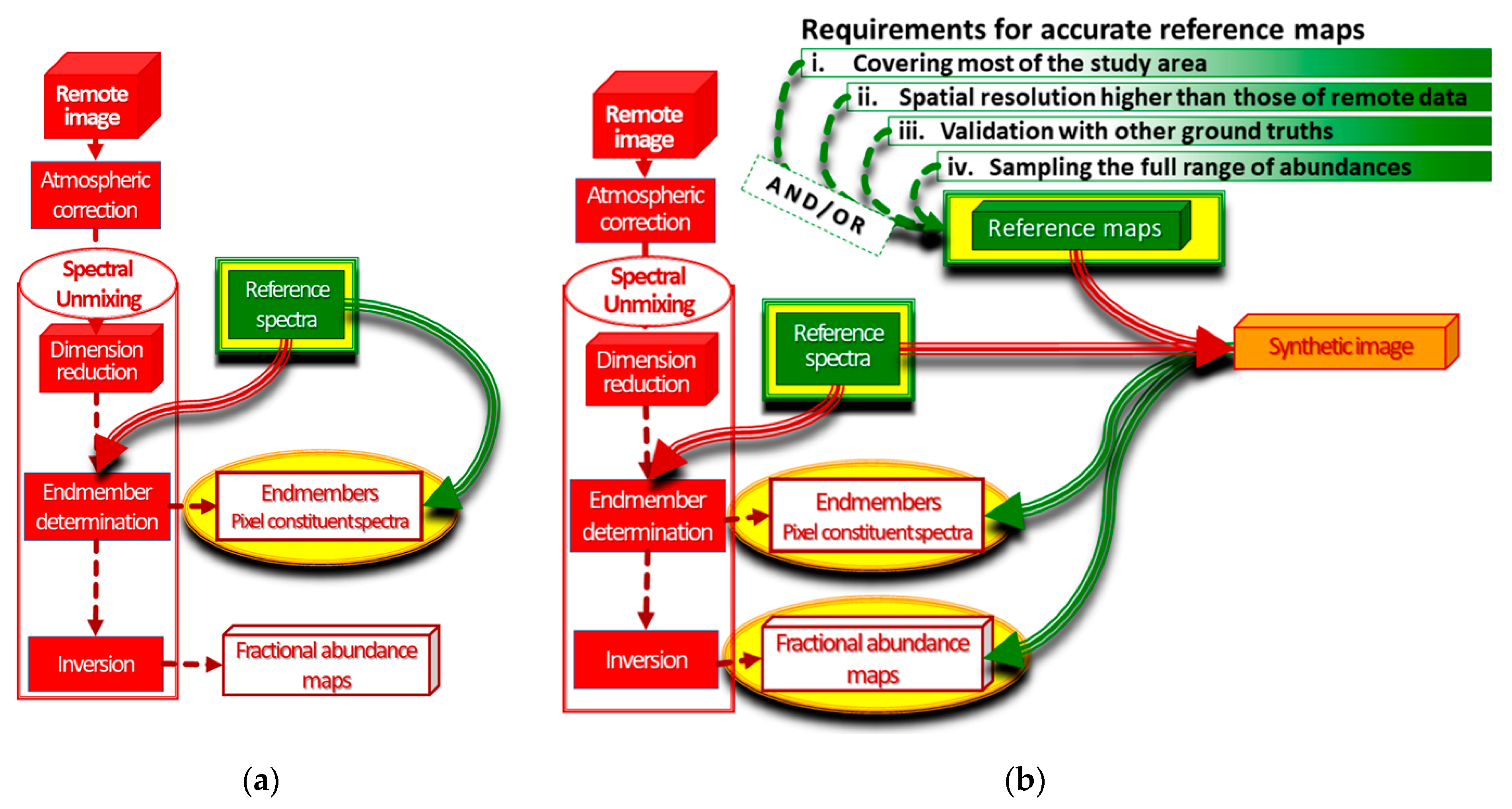
Figure 2.
The flowcharts of spatial validation methods.
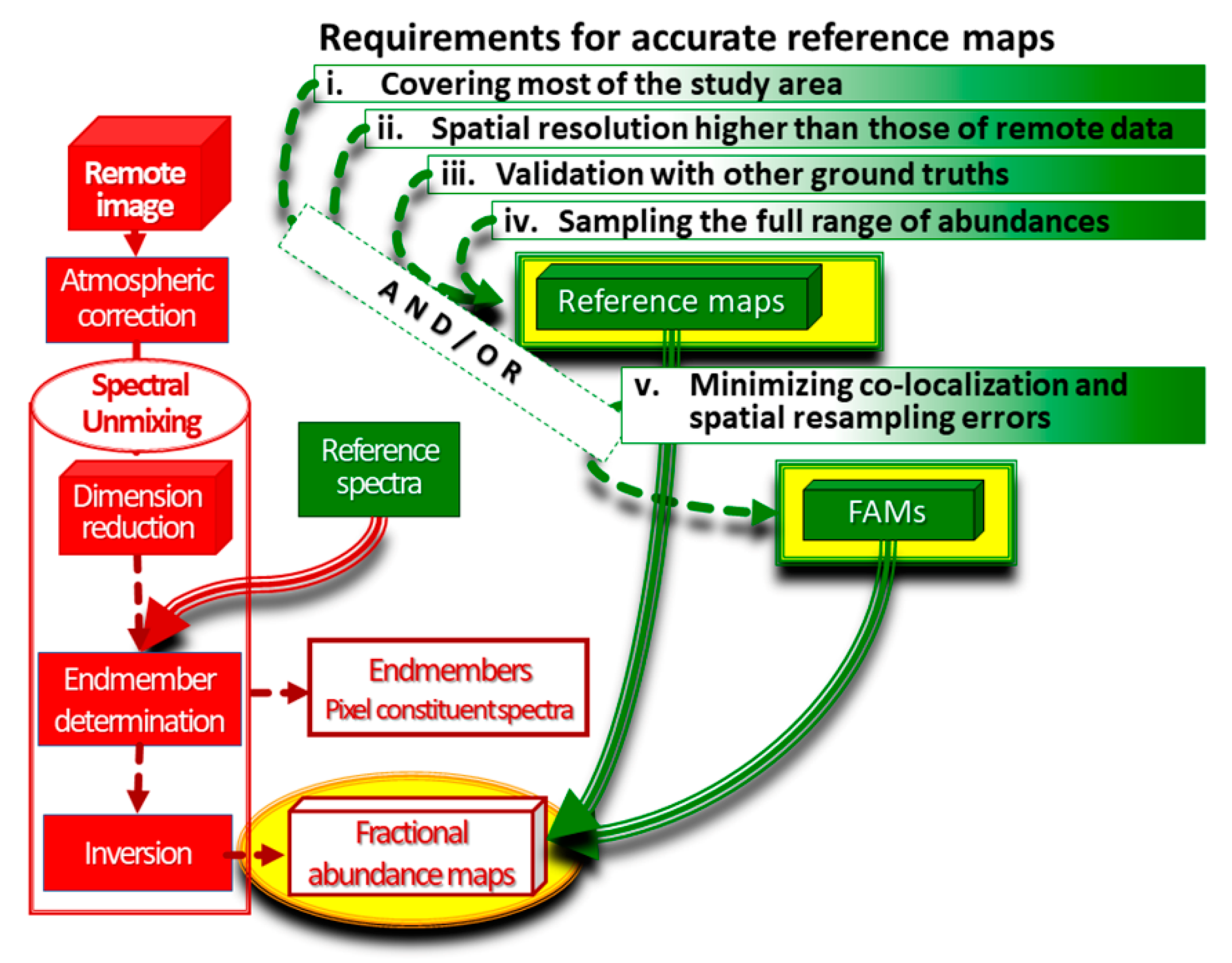
Figure 3.
Study area: (a) study area location (red square); (b) IKONOS image of study area.
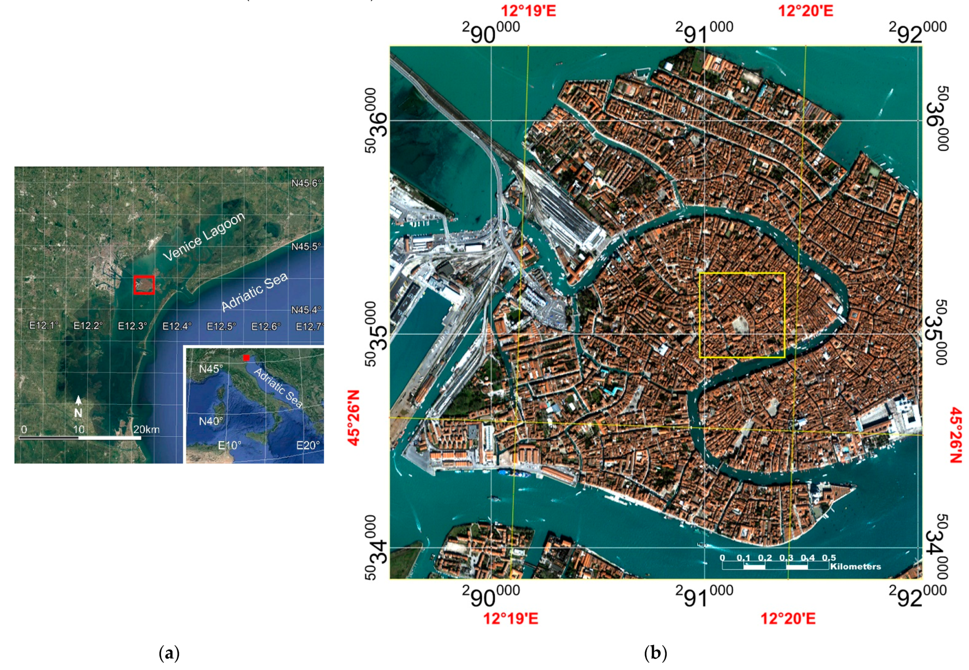

Figure 5.
The procedure of fractional abundance determining applied to trachyte endmember is shown: (a) the validated reference map at 0.20 m (green) superimposed on the previous reference map (white); (b) the pixels with 100% abundance (red) superimposed on the validated reference map (white); (c) reference fractional abundance map determined only for areas surrounding those with 100% abundance; colors with corresponding percentages are shown on the right; (d) the completed reference fractional abundance map highlighted with a color ramp; colors with corresponding percentages are shown on the right.
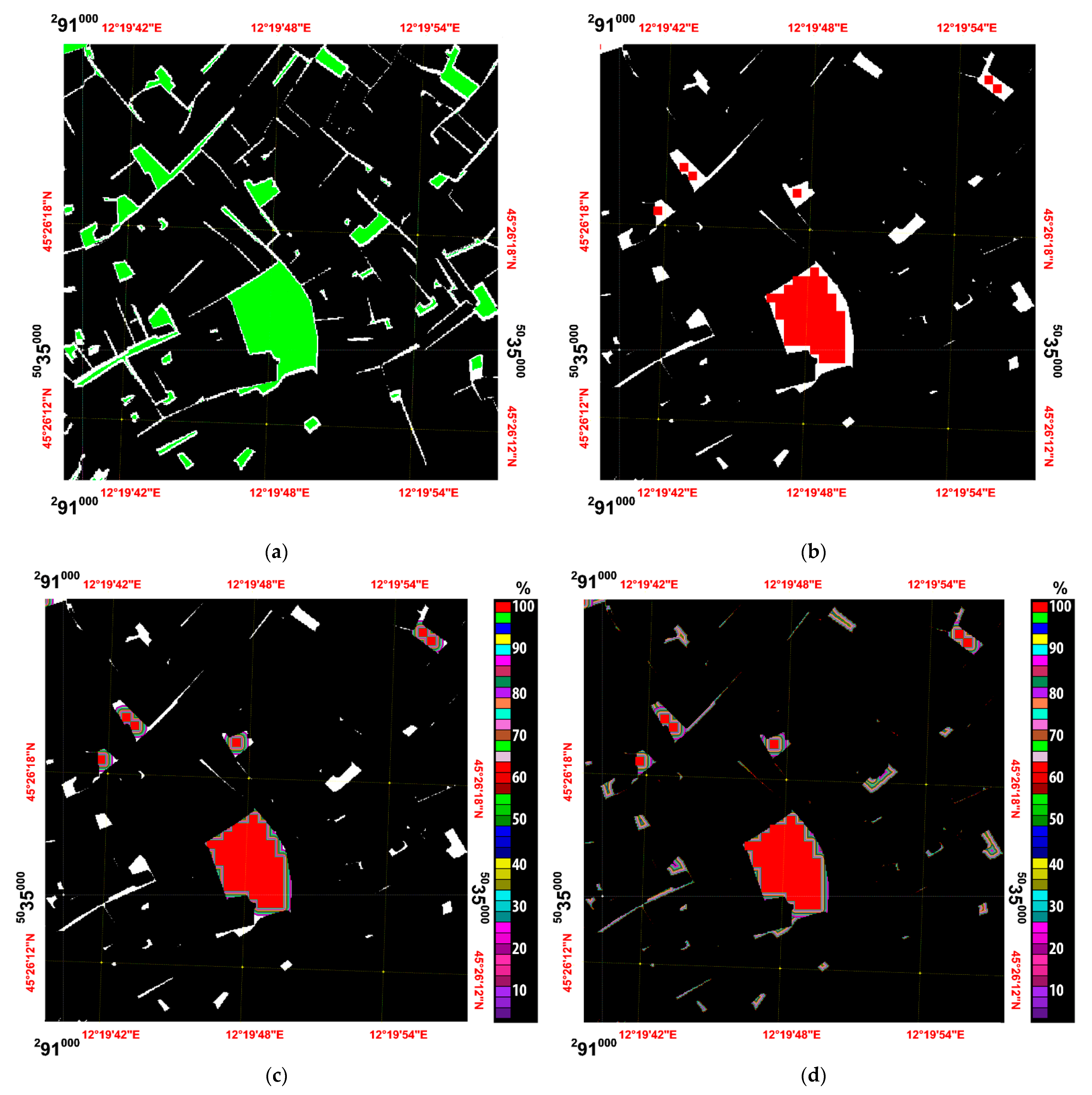
Figure 6.
Comparison of image-resampling methods; first, methods used to resample the reference mask from 0.20 to 8 m, and second, those used to resample from 8 to 0.20 m: (a) first, the nearest neighbor method and, second, the bilinear convolution method were applied; (b) first, the nearest neighbor method and, second, the cubic convolution method were applied; (c) first, the nearest neighbor method and, second, the nearest neighbor method were applied; (d) first, the pixel aggregate method and, second, the bilinear convolution method were applied; (e) first, the pixel aggregate method and, second, the cubic convolution method were applied; (f) first, the pixel aggregate method and, second, the nearest neighbor method were applied.
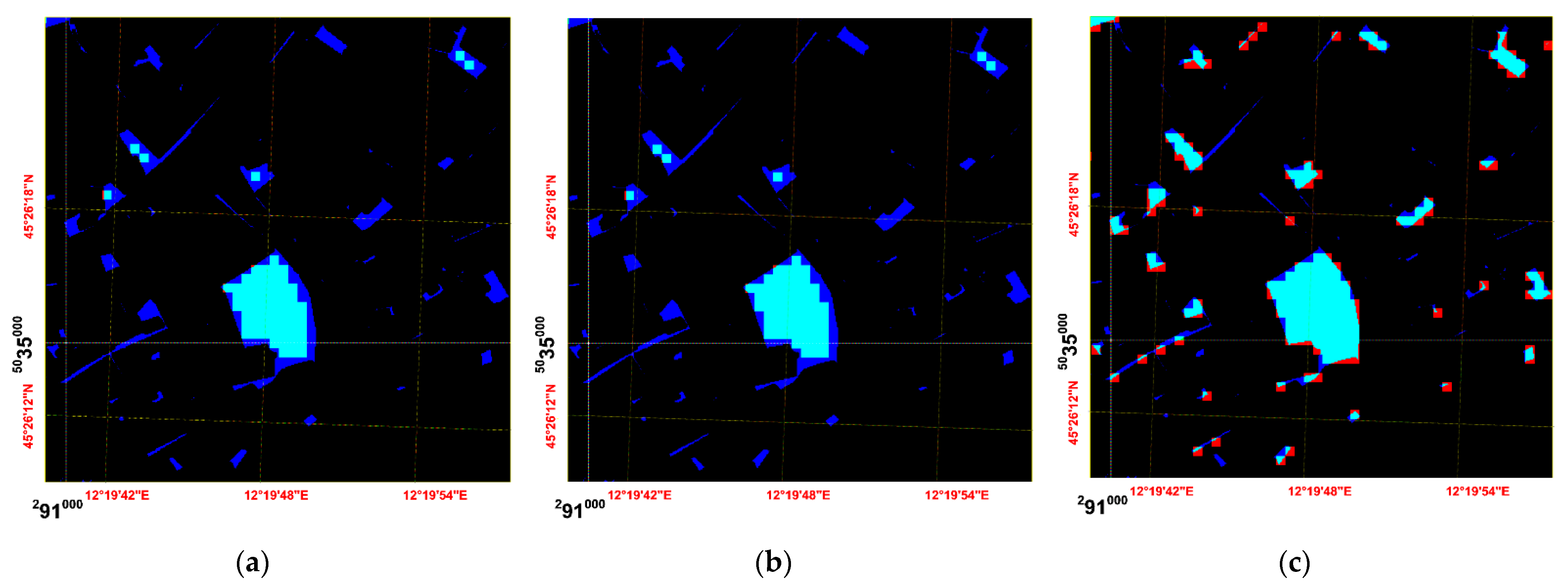
Figure 7.
The flowcharts of the validation methods: (a) the second method; (b) the third method; (c) the fourth method; (d) the fifth method.
Figure 7.
The flowcharts of the validation methods: (a) the second method; (b) the third method; (c) the fourth method; (d) the fifth method.
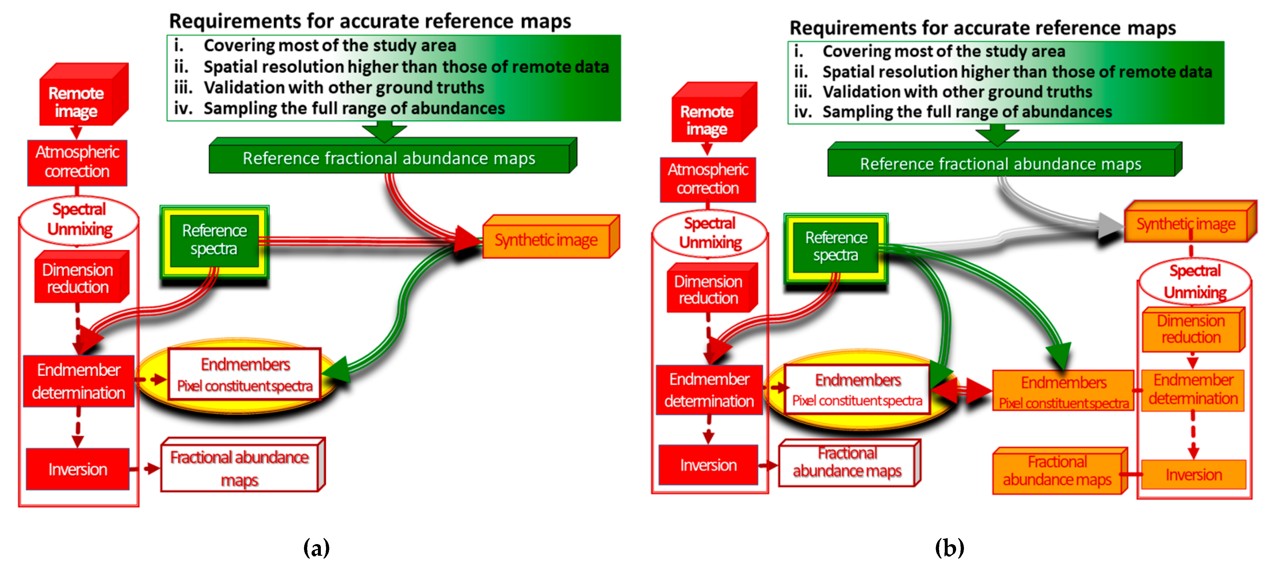
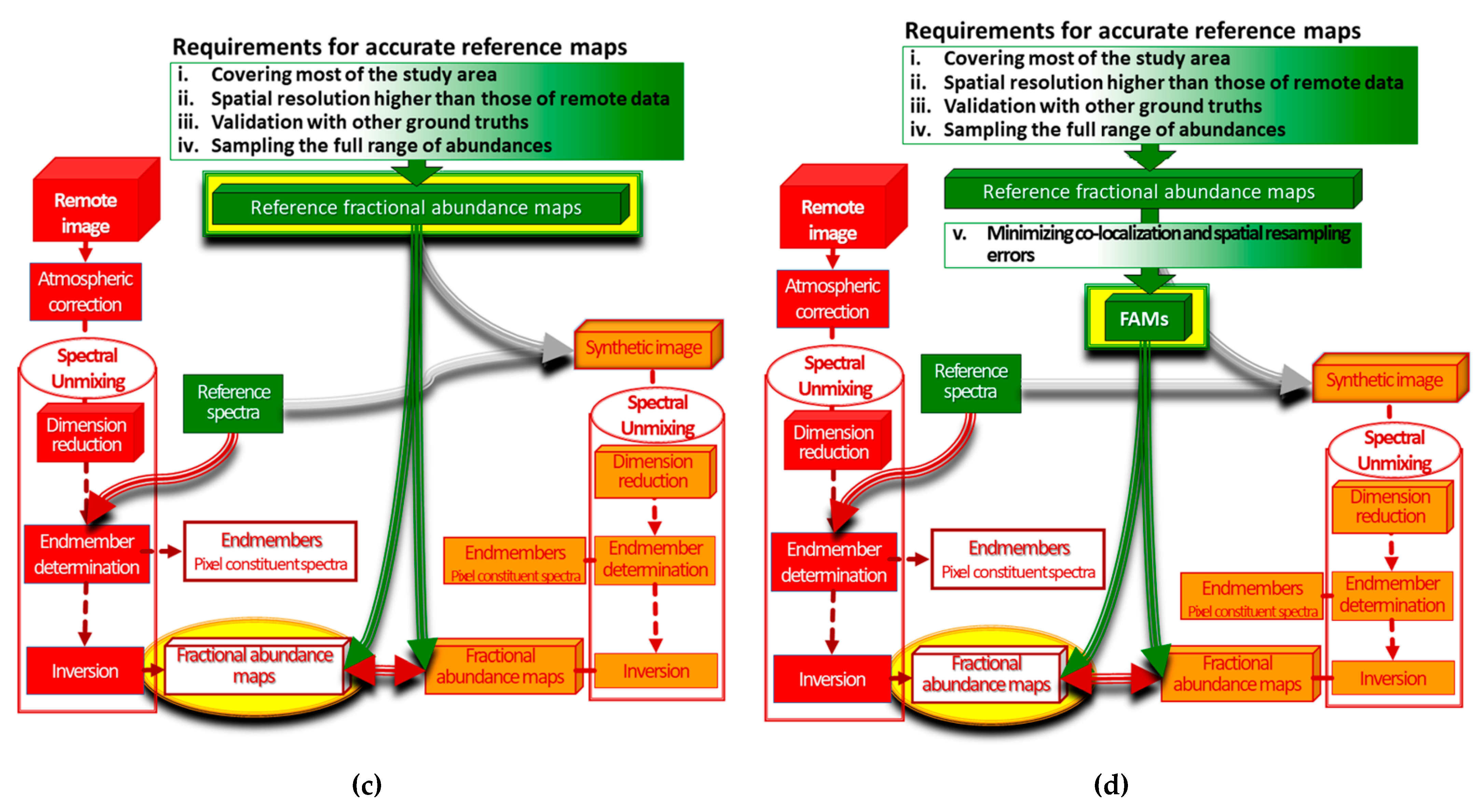
Figure 8.
FAMs: (a) FAMs of Lateritic tiles, Lead plates, and Vegetation; (b) FAM of Asphalt, Limestone, and Trachyte rock.
Figure 8.
FAMs: (a) FAMs of Lateritic tiles, Lead plates, and Vegetation; (b) FAM of Asphalt, Limestone, and Trachyte rock.

Figure 9.
RMSk values obtained from true and synthetic images of MIVIS.
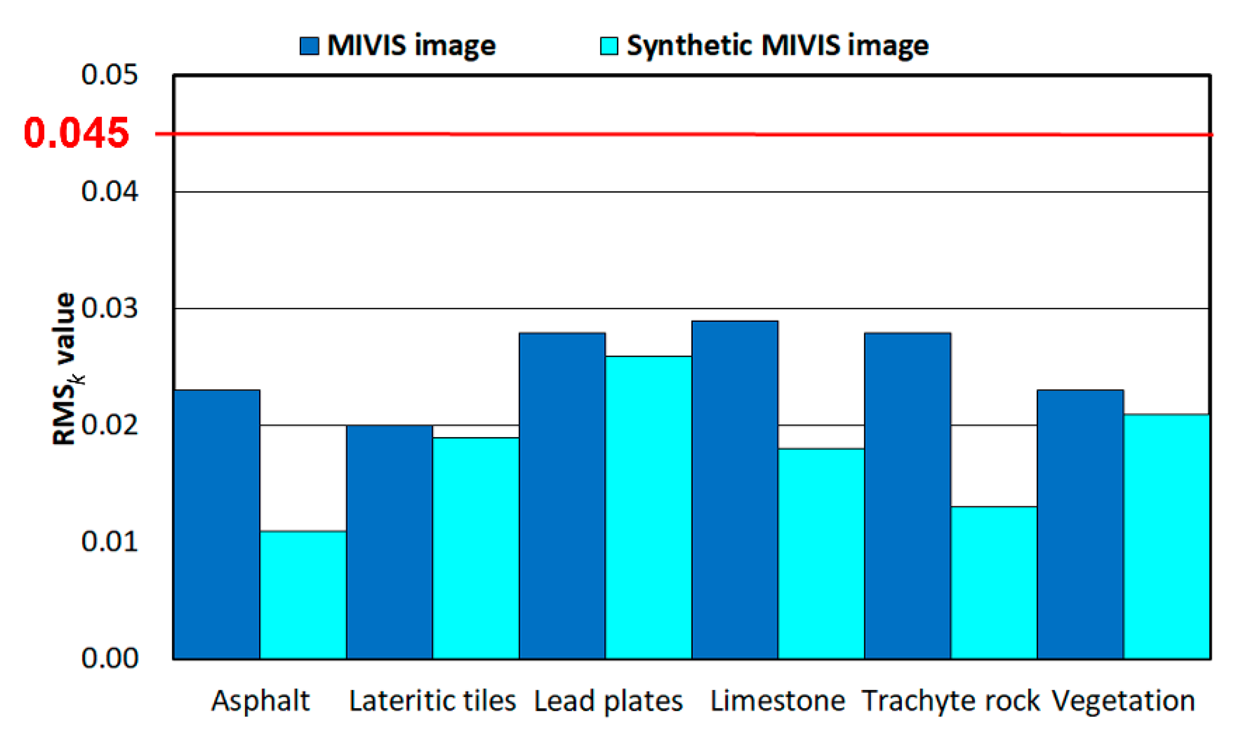
Figure 10.
The percentage of RMSk values due to the spatial and spectral characteristics of the MIVIS image, the reference endmember set and LMM.
Figure 10.
The percentage of RMSk values due to the spatial and spectral characteristics of the MIVIS image, the reference endmember set and LMM.

Figure 11.
MAEk-100–50% and MAEk-49–0% values obtained from true and synthetic images.

Figure 12.
The percentage of MAEk-Totals values related to the spatial and spectral characteristics of and MIVIS image, the reference endmember set and LMM.
Figure 12.
The percentage of MAEk-Totals values related to the spatial and spectral characteristics of and MIVIS image, the reference endmember set and LMM.
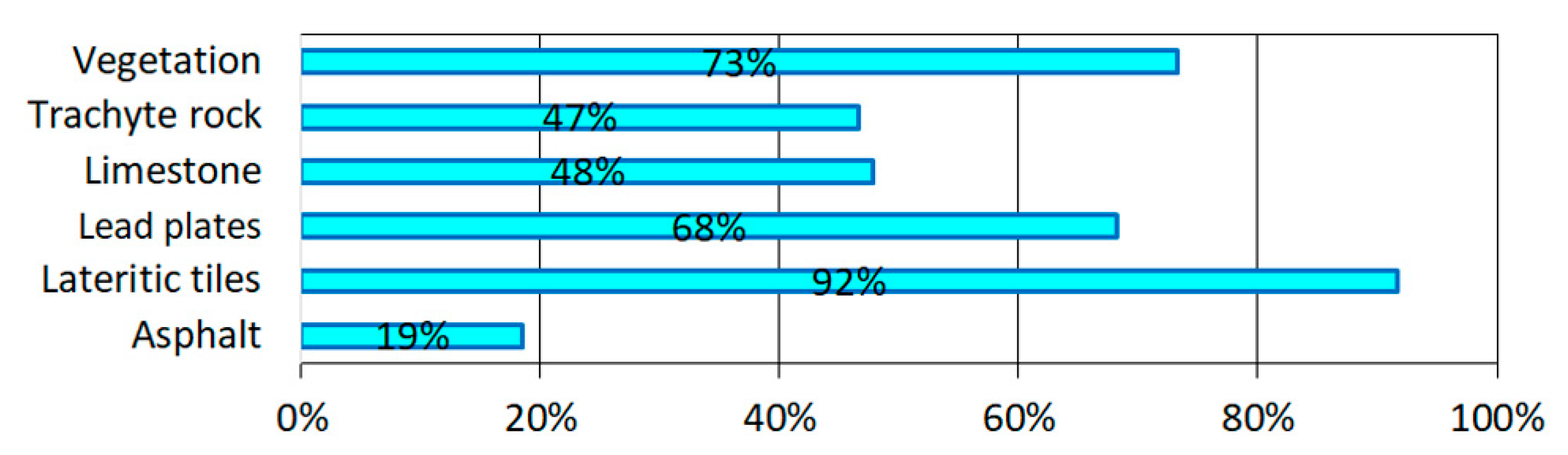
Figure 13.
The error in spatial validation calculated from true and synthetic images exploiting FAMs (i.e., the fifth method).
Figure 13.
The error in spatial validation calculated from true and synthetic images exploiting FAMs (i.e., the fifth method).
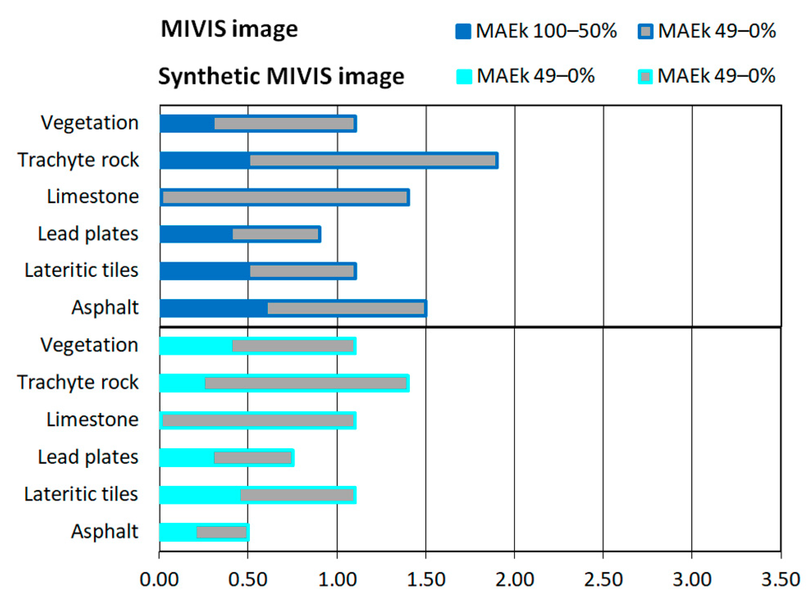

Table 1.
Requirements for accurate reference maps.
| Requirements for Accurate Reference Maps | Proposed by | Met by | |
|---|---|---|---|
| I° requirement | Covering most of the study area | [6] | Most of the authors |
| II° requirement | Spatial resolution higher than those of remote data | [18,37] | Most of the authors |
| III° requirement | Validation with other ground truths | [36,38,39] | [36,38,39] |
| IV° requirement | Sampling the full range of abundances | [12,33,37,39] | [12,33,37,39] |
| V° requirement | Minimizing co-localization and spatial resampling errors | [33] | [33] |
Table 2.
Characteristics of the MIVIS image.
| KERRYPNX | Spatial Resolution (m) | Bands | Spectral Region | Spectral Resolution (μm) | Spectral Range (μm) |
|---|---|---|---|---|---|
| MIVIS | 8 | 20 | VIS | 0.02 | 0.4–0.83 |
| 8 | NIR | 0.05 | 1.15–1.55 | ||
| 64 | SWIR | 0.09 | 2–2.5 | ||
| 10 | TIR | 0.34–0.54 | 8.2–12.7 |
Table 3.
The metrics performed to evaluate the spatial and spectral accuracy in the five methods.
| Spectral Validation Methods | Reference Data Employed | Accuracy of the Pixel Constituent Spectra | |
| Error Measure | Similarity Measure | ||
| First (Figure 1a) | Reference spectra | RMSk | SADk—aSSMnk |
| Second (Figure 7a) | Spectra of synthetic image | SADk—aSSMnk | |
| Third (Figure 7b) | Pixel constituent spectra obtained from synthetic image | RMSk | |
| Spatial Validation Methods | Reference Data Employed | Accuracy of the Fractional Abundance Maps | |
| Error Measure | Similarity Measure | ||
| Fourth (Figure 7c) | Reference fractional abundance maps and fractional abundance maps obtained from synthetic image | MAEk | |
| Fifth (Figure 7d) | FAMs and fractional abundance maps obtained from synthetic image | MAEk | KGE |
Table 4.
In the first and third methods, spectral accuracy estimated with RMSk values that were retrieved from true and synthetic images of MIVIS and the absolute differences between the RMSk values obtained from true and synthetic image (ΔRMSk).
Table 4.
In the first and third methods, spectral accuracy estimated with RMSk values that were retrieved from true and synthetic images of MIVIS and the absolute differences between the RMSk values obtained from true and synthetic image (ΔRMSk).
| MIVIS Image | Synthetic MIVIS Image | ||
|---|---|---|---|
| Endmembers | RMSk | RMSk | ΔRMSk |
| Asphalt | 0.023 | 0.011 | 0.012 |
| Lateritic tiles | 0.020 | 0.019 | 0.000 |
| Lead plates | 0.028 | 0.026 | 0.002 |
| Limestone | 0.029 | 0.018 | 0.011 |
| Trachyte rock | 0.028 | 0.013 | 0.015 |
| Vegetation | 0.023 | 0.021 | 0.002 |
Table 5.
In the second method, spectral accuracy estimated with SADk, σSADk, aSSMnk, and σaSSMnk values that were retrieved from true and synthetic images and the absolute differences between SADk, σSADk, aSSMnk, and σaSSMnk values obtained from true and synthetic images (ΔSADk, ΔσSADk, ΔaSSMnk, and Δ σaSSMnk).
| MIVIS Image | ||||
|---|---|---|---|---|
| Endmembers | SADk | σSADk | aSSMnk | σaSSMnk |
| Asphalt | 0.361 | 0.123 | 0.558 | 0.395 |
| Lateritic tiles | 0.299 | 0.069 | 0.659 | 0.255 |
| Lead plates | 0.282 | 0.079 | 0.693 | 0.247 |
| Limestone | 0.379 | 0.129 | 0.498 | 0.423 |
| Trachyte rock | 0.387 | 0.143 | 0.485 | 0.417 |
| Vegetation | 0.361 | 0.083 | 0.677 | 0.251 |
| Synthetic MIVIS Image | ||||
| Endmembers | SADk | σSADk | aSSMnk | σaSSMnk |
| Asphalt | 0.282 | 0.060 | 0.653 | 0.293 |
| Lateritic tiles | 0.271 | 0.042 | 0.772 | 0.217 |
| Lead plates | 0.253 | 0.065 | 0.714 | 0.245 |
| Limestone | 0.286 | 0.035 | 0.581 | 0.245 |
| Trachyte rock | 0.281 | 0.062 | 0.649 | 0.312 |
| Vegetation | 0.302 | 0.051 | 0.718 | 0.195 |
| Endmembers | ΔSADk | ΔσSADk | ΔaSSMnk | ΔσaSSMnk |
| Asphalt | 0.079 | 0.063 | 0.095 | 0.102 |
| Lateritic tiles | 0.028 | 0.027 | 0.113 | 0.038 |
| Lead plates | 0.029 | 0.014 | 0.021 | 0.002 |
| Limestone | 0.093 | 0.094 | 0.083 | 0.178 |
| Trachyte rock | 0.106 | 0.081 | 0.164 | 0.105 |
| Vegetation | 0.059 | 0.032 | 0.041 | 0.056 |
Table 6.
The error in co-localization and spatial resampling evaluated by MIVIS image processing with ErrorTotal, Error100–50%, and Error49–0% values.
Table 6.
The error in co-localization and spatial resampling evaluated by MIVIS image processing with ErrorTotal, Error100–50%, and Error49–0% values.
| MIVIS Image | |||
|---|---|---|---|
| Endmembers | ErrorTotals | Error100–50% | Error49–0% |
| Asphalt | 44.4% | 33.3% | 50.0% |
| Lateritic tiles | 8.3% | 16.7% | 0.0% |
| Lead plates | 18.2% | 20.0% | 16.7% |
| Limestone | 39.1% | 0.0% | 39.3% |
| Trachyte rock | 36.7% | 0.0% | 44.0% |
| Vegetation | 26.7% | 25.0% | 27.3% |
Table 7.
In the fifth method, spatial accuracy is measured with KGE values that were obtained from true and synthetic images and the absolute difference between these values.
Table 7.
In the fifth method, spatial accuracy is measured with KGE values that were obtained from true and synthetic images and the absolute difference between these values.
| MIVIS Image | |||
|---|---|---|---|
| True | Synthetic | Difference | |
| Endmembers | KGE | KGE | KGE |
| Asphalt | −0.010 | 0.050 | 0.060 |
| Lateritic tiles | 0.150 | 0.315 | 0.165 |
| Lead plates | 0.170 | 0.720 | 0.550 |
| Limestone | −0.060 | 0.012 | 0.072 |
| Trachyte rock | −0.080 | −0.028 | 0.052 |
| Vegetation | 0.300 | 0.485 | 0.185 |
Publisher’s Note: MDPI stays neutral with regard to jurisdictional claims in published maps and institutional affiliations. |
© 2022 by the author. Licensee MDPI, Basel, Switzerland. This article is an open access article distributed under the terms and conditions of the Creative Commons Attribution (CC BY) license (https://creativecommons.org/licenses/by/4.0/).
Share and Cite
MDPI and ACS Style
Cavalli, R.M. Spatial Validation of Spectral Unmixing Results: A Case Study of Venice City. Remote Sens. 2022, 14, 5165. https://doi.org/10.3390/rs14205165
AMA Style
Cavalli RM. Spatial Validation of Spectral Unmixing Results: A Case Study of Venice City. Remote Sensing. 2022; 14(20):5165. https://doi.org/10.3390/rs14205165
Chicago/Turabian StyleCavalli, Rosa Maria. 2022. "Spatial Validation of Spectral Unmixing Results: A Case Study of Venice City" Remote Sensing 14, no. 20: 5165. https://doi.org/10.3390/rs14205165
Note that from the first issue of 2016, this journal uses article numbers instead of page numbers. See further details here.