
UAV Remote Sensing Prediction Method of Winter Wheat Yield Based on the Fused Features of Crop and Soil
by
 , ,
, ,
Zezhong Tian
1,
Yao Zhang
1,*,
Kaidi Liu
1,
Zhenhai Li
2,
Minzan Li
1,
Haiyang Zhang
1 and
Jiangmei Wu
1 1
Key Laboratory of Smart Agriculture System Integration Research of Ministry of Education, China Agricultural University, Beijing 100083, China
2
Key Laboratory of Quantitative Remote Sensing in Ministry of Agriculture and Rural Affairs, Information Technology Research Center, Beijing Academy of Agriculture and Forestry Sciences, Beijing 100097, China
*
Author to whom correspondence should be addressed.
Remote Sens. 2022, 14(19), 5054; https://doi.org/10.3390/rs14195054
Submission received: 20 August 2022
/
Revised: 30 September 2022
/
Accepted: 4 October 2022
/
Published: 10 October 2022
(This article belongs to the Topic Applications of Big Data and Machine Learning in Smart Agriculture)
Abstract
:The early and accurate acquisition of crop yields is of great significance for maintaining food market stability and ensuring global food security. Unmanned aerial vehicle (UAV) remote sensing offers the possibility of predicting crop yields with its advantages of flexibility and high resolution. However, most of the existing remote sensing yield estimation studies focused solely on crops but did not fully consider the influence of soil on yield formation. As an integrated system, the status of crop and soil together determines the final yield. Compared to crop-only yield prediction, the approach that additionally considers soil background information will effectively improve the accuracy and reduce bias in the results. In this study, a novel method for segmenting crop and soil spectral images based on different vegetation coverage is first proposed, in which pixels of crop and soil can be accurately identified by determining the discriminant value Q. On the basis of extracting crop and soil waveband’s information by individual pixel, an innovative approach, projected non-negative matrix factorization based on good point set and matrix cross fusion (PNMF-MCF), was developed to effectively extract and fuse the yield-related features of crop and soil. The experimental results on winter wheat show that the proposed segmentation method can accurately distinguish crop and soil pixels under complex soil background of four different growth periods. Compared with the single reflectance of crop or soil and the simple combination of crop and soil reflectance, the fused yield features spectral matrix FP obtained with PNMF−MCF achieved the best performance in yield prediction at the flowering, flag leaf and pustulation stages, with R2 higher than 0.7 in these three stages. Especially at the flowering stage, the yield prediction model based on PNMF-MCF had the highest R2 with 0.8516 and the lowest RMSE with 0.0744 kg/m2. Correlation analysis with key biochemical parameters (nitrogen and carbon, pigments and biomass) of yield formation showed that the flowering stage was the most vigorous season for photosynthesis and the most critical stage for yield prediction. This study provides a new perspective and complete framework for high-precision crop yield forecasting using UAV remote sensing technology.
1. Introduction
As one of the world’s most important food crops, wheat is consumed as a staple food by more than a third of the global population [1,2]. In recent years, food security is becoming the most challenging topic globally due to the recurrence of COVID-19 and the intensification of regional conflicts [3]. Accurate food production forecasts are of great importance to maintain food market stability and ensure global food security [4,5].
The traditional methods of yield prediction are mainly through field surveys, which are inefficient and destructive to crops [6]. With the diversification of remote sensing (RS) platforms and the improvement of data access quality [7], RS technology has been recognized as an effective method for crop yield prediction [8]. In the past decades, satellite RS technology has been widely used for large-scale agricultural monitoring [9,10]. However, its application is hampered by satellite revisit cycles and complicated weather conditions, such as clouds and rain [11]. Unmanned aerial vehicle (UAV) RS has the advantages of high flexibility and mobility, which can quickly and effectively acquire high spatial resolution RS images in the farmland scale [12,13].
However, most yield RS studies based on UAV platforms do not consider differentiating crop and soil pixels [13,14,15]. Obviously, when extracting the spectral information from targeted study areas for crop yield prediction studies, the neglect of the soil background will inevitably decrease the prediction results [16]. Therefore, the segmentation of crop and soil in the targeted images is the first and very important step in farmland yield prediction [17,18]. The main crop and soil segmentation methods currently are color index-based, learning-based and threshold-based segmentation [19]. However, color index-based methods are not accurate enough [20], and learning-based methods have high training costs and low universality [21]. The accuracy of segmentation using threshold-based methods is easily influenced by variations of the light environment and vegetation covers [19]. To date, there is no definitive and quantitative crop and soil segmentation method applicable to different periods and scenarios. Therefore, there is an urgent need for a high-precision segmentation method for crop and soil under different light environments and different cover conditions, which is the key and basis for realizing pixel-level accurate extraction and fusion applications of crop and soil multispectral information in farmland UAV images.
In addition, the nutrient changes in soils are closely related to crop yield [22,23]. However, the existing remote sensing yield estimation methods are mostly from the crop perspective only, ignoring the influence of soil information on yield formation [24,25,26]. Different from crop yield research that excludes soil background, yield studies that comprehensively consider crop and soil are more consistent with the mechanism of yield formation and can reduce yield errors caused by only studying crops [27,28]. Therefore, how to fully exploit and integrate soil and crop information, and further improve the accuracy of yield estimation is another urgent problem to be solved.
In order to achieve high-precision yield estimation with the effective fusion of crop and soil spectral features, accurately identifying crop and soil pixels and extracting spectral information under different vegetation coverages and light conditions is an important step. Focusing on the above objectives, this study firstly proposes a discriminant Q, constructed based on crop spectral features by preserving the difference between red edge and red and attenuating the difference between NIR and red edge, which can effectively identify crop and soil pixels under complex and variable vegetation coverages and light conditions in agricultural fields. On the basis of the precise segmentation of crop and soil pixels, a new method based on the Projected Nonnegative Matrix Factorization (PNMF) [29], optimized by Good Point Set theory [30], named PNMF−MCF is proposed, which can effectively extract and fuse the yield features of crop and soil. This study will provide a feasible solution for using RS techniques to accurately segment crop and soil pixels and predict yield by fusing crop and soil spectral features.
The paper is organized as follows. Section 2 introduces the experiment designs in this study and a detailed description regarding the proposed crop and soil segmentation method, and the crop and soil spectral yield features fusion method called PNMF−MCF. The results of crop and soil spectral image segmentation and crop yield prediction are presented in Section 3. The comparison of the proposed segmentation method with other methods based on HSV and Deep Learning, the influence of fused parameters on yield predictive performance of PNMF−MCF, the correlation between fused matrix FP and other physiological parameters are discussed in Section 4. The paper concludes in Section 5 with a summary of the results.
2. Materials and Methods
2.1. Experiment Design
The experimental site was National Station for Precision Agriculture (116.4°E, 40.2°N) in Beijing, China, which has a temperate monsoon climate with brown soil and moderate humus content [31]. Winter wheat was planted on 29 September 2020 and harvested on 17 June 2021. The brown soil had a nitrate nitrogen content ranging from 3.16 to 14.82 mg/kg, ammonium nitrogen content ranging from 8.2 to 14.52 mg/kg, fast-acting potassium content ranging from 86.83 to 120.62 mg/kg, effective phosphorus content ranging from 3.14 to 21.18 mg/kg, and soil organic matter content ranging from 15.8 to 20.0 g/kg in the 0–0.3 m soil layers.
The field experiment was conducted in the jointing stage (9 April), flag leaf stage (25 April), flowering stage (11 May), and pustulation stage (26 May) in 2021. To increase the difference in winter wheat growth, two winter wheat varieties, Jinghua 11 (P1) and Zhongmai 1062 (P2), were planted in 32 experimental plots (135 m2 each). The four urea fertilization levels for each variety were N0 (0 kg/hm2), N1 (195 kg/hm2), N2 (390 kg/hm2) and N3 (585 kg/hm2). Three irrigation levels were W0 (Natural Rainwater), W1 (148 mm) and W2 (271 mm). Set 1 m buffer strip in the interval regions to eliminate mutual influence and four replicates for each plot. A sample area of 1 m2 within each plot was selected for the segmentation of crop and soil pixels, fusion of yield feature spectral matrix and the final yield determination. The experimental site is shown in Figure 1.
Data Acquisition
The spatial resolution and spectral resolution are constrained by each other and because of the requirement of pixel-level image segmentation in this study. The DJI Phantom 4 UAV (DJI, Inc., Shenzhen, Guangdong, China) carrying six CMOS sensors was selected. The UAV weighs 1375 g; has a 350 mm wheelbase, a maximum flight time of 28 min and a maximum flight speed of 20 m/s; and carries a GPS/GLONASS satellite positioning module. The UAV’s sensors include an RGB sensor for visible imaging and five single-band sensors for multispectral imaging, each with 2.08 million effective pixels. The five sensors for multispectral imaging are centered at 450, 560, 650, 730 and 840 nm, respectively, with a lens FOV of 94° 8.8 mm/24 mm. JPEG (visible imaging) + TIFF (multispectral imaging) images with a maximum resolution of 1600 × 1300 pixels can be captured.
The DJI Phantom 4 UAV carried the camera to take the area multispectral images at 30 m altitude on four growth stages, which correspond to the spatial resolution of 1.5 cm. The UAV heading overlap was 80% and the side overlap was 70%, and the waypoints were marked in DJI Terra software to generate S-shaped routes. The radiometric calibration was performed using a MAPIR standard calibration plate, which carries four diffuse reflectance plates with different reflectance. Before takeoff, the calibration plate was placed flat on the ground, and the UAV’s lens was manually controlled to shoot vertically downward to ensure no shadows were on the calibration plate. The co-registration, geometric correction, radiometric calibration and band alignment of the UAV multispectral image data were all conducted in DJI Terra software (V3.5.5).
At harvest time, all crop ears collected in 1 m2 sample area from each plot were heated to 105 Celsius until they reached a constant weight in the laboratory [4]. The dried grain was then manually collected from the ear and the final dry weight of the grain in kilograms was recorded. In addition, in each 1 m2 sample area at the four growth stages before harvest, the nitrogen content of crop and soil, the carbon content of crop and soil, the chlorophyll A and chlorophyll B contents, carotenoid content and the crop biomass were measured. The measurement methods were according to references [32,33,34,35] and Table 1.
2.2. Crop and Soil Piecewise Segmentation Method
Crop and soil, as the most important components of farmland, are the two most fundamental factors for yield estimation [36]. The accurate segmentation of crop and soil on spectral images is the key step for making full use of crop and soil spectral information [16]. Crop-specific spectral characteristics, a sharp increase from the red band to the Near-Infrared (NIR) band, is a key characteristic in differentiating from soil [36,37,38], which makes NDVI a commonly used indicator for crop identification [39]. However, in complex and variable farming conditions, there is no fixed evaluation standard to determine the NDVI value that can distinguish crop from soil, and the segmentation function of NDVI will fail due to NDVI saturation under high vegetation coverage [40].
To address the above problems, this study proposes a piecewise segmentation method for crop and soil, which includes two steps: vegetation coverage determination and threshold fine discrimination.
2.2.1. Vegetation Coverage Determination Function
In order to determine a quantitative value to judge the vegetation coverage under different growth conditions and different growth periods, a general vegetation coverage determination function is proposed as Equation (1). Kv represents the vegetation coverage level. If Kv ≥ 1, the area is considered as high vegetation coverage. Otherwise, the area is considered as a low vegetation coverage. For most cases, this function takes into account the NDVI of all pixels within the targeted scene. Thus, it can ensure the accurate segmentation of crop and soil in different growing environments.
where NAVG is the average value of NDVI of all pixels in the targeted images, NMIN wisas the minimum value of NDVI and NMAX is the maximum value of NDVI.
2.2.2. Discriminant Value Q for the Segmentation of Crop and Soil
The large fluctuations in NDVI values caused by different vegetation coverage make it impossible to distinguish crop and soil with a fixed value in variable farming situations. Therefore, the discriminant value Q introducing vegetation cover information was proposed to further achieve the pixel-level crop and soil precision segmentation suitable for complex farming conditions with a fixed discriminant value.
The discriminant value Q that includes red, red edge and NIR was proposed to distinguish crop and soil, as shown in Equation (2).
where RED, EDGE and NIR are the reflectance of the pixel at 650 nm, 730 nm and 840 nm, respectively.
Usually at low vegetation coverage, Kv is lower than 1, while at high vegetation coverage, Kv is higher than 1. Therefore, it can be found from Equation (2) that, on the basis of maintaining the difference between red edge and near infrared, the addition of Kv in denominator diminishes the difference between red and red edge. That means the introduction of Kv weakens the disturbance caused by different vegetation covers to crop and soil segmentation, so that the discriminant value Q can segment crop and soil under different vegetation coverages with a fixed value.
The multispectral images were traversed in a 5 × 5 pixel size window. In each window, the maximum, average and minimum of NDVI of all pixels were selected, and then the vegetation coverage index Kv was calculated according to Equation (1). Based on the Kv and three wavebands (red, red edge and NIR) information, the discriminant Q of every pixel was calculated. It was determined by visual interpretation that crops and soils can be effectively distinguished when Q is 0.1. In addition, after extensive validation tests, the threshold segmentation with Q of 0.1 has strong stability under different vegetation covers and light conditions. If the discriminant value Q for this pixel is greater than or equal to 0.1, the pixel is judged to be winter wheat. Otherwise, the pixel is judged to be soil.
2.2.3. Accuracy Evaluation for Crop and Soil Segmentation
To verify the accuracy of the segmentation results more precisely, the intersection of union (IoU) [41] was used as an evaluation metric for the accuracy of segmentation. IoU consists of precision and recall, where precision is the proportion of the number of correct pixels among the target pixels identified by the algorithm, and recall is the proportion of the number of correct pixels identified by the algorithm to the total number of real pixels. IOU includes all possible cases of binary identification (A is identified as A, A is identified as B, B is identified as B, and B is identified as A) and is well suited for judging the accuracy of crop and soil segmentation. The closer the IoU is to 1, the higher the identification accuracy of the target pixel. The calculation of IoU is shown in Equation (3).
where TrueP is the number of pixels (crop or soil) that are correctly identified, FalseP is the number of pixels (crop or soil) that are incorrectly identified FalseN is the number of pixels in another category (soil or crop) that are incorrectly identified.
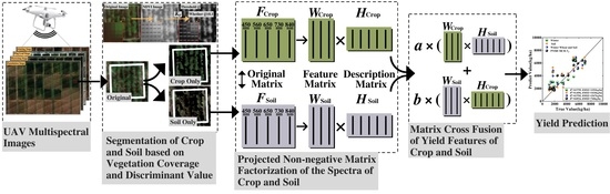
2.3. Projected Non-Negative Matrix Factorization and Matrix Cross Fusion
After the accurate segmentation of farm crop and soil, the next step is to further mine and fuse the information of the two targets. Therefore, a method combining Projected Non-negative Matrix Factorization optimized by Good Point Set (GPS) and Matrix Cross Fusion (PNMF-MCF) is proposed in this study, and the flow chart of the method is shown in Figure 2.
2.3.1. Matrix Initialization Based on Good Point Set
The theory of Good Point Set [30] was first proposed by Hua Luogeng. According to the definition of GPS, is a unit cube in s-dimensional Euclidean space, The point set is composed of n points in For any given point in m is the number of points that satisfies the following inequality (4).
The deviation is defined in Equation (5).
If the deviation of satisfies , where is a positive constant related only to and , is an arbitrarily small positive number, is considered as a good set of points and is called a good point, then the good point can be calculated based on cyclotomic field method as shown in Equation (6).
where t is the minimum prime number that satisfies .
According to the above definition, if n points are taken randomly in the s-dimensional space, the deviation is o(n−1/2). While n points are taken by the good point set method, the deviation is o(). The deviation of latter is much smaller, which is why the good point set amount data converge faster.
2.3.2. Projected Non-Negative Matrix Factorization Optimized by Good Point Set
Non-negative matrix factorization [42] ensures matrix elements are always positive, which is suitable for spectroscopic analysis. Given a non-negative initial spectral matrix and a positive integer l, factorize into a non-negative matrix W and a non-negative matrix H, as shown in Formula (7).
where W is the basis feature matrix of V and H is the weighting coefficients matrix.
Lin proposed an improved algorithm Projected Non-negative Matrix Factorization (PNMF) based on projection gradient and Armijo [43] proposed step size rule, which makes the algorithm converge more easily and faster [29]. (The detailed mathematical model about PNMF is shown in the Appendix A) However, both the original and improved NMF algorithms suffer from the problem that the result of each factorization is not unique and, therefore, the application is difficult. This is because the initial matrix is generated randomly, so the matrix initialization based on GPS is adopted in PNMF to improve the factorization result and make the result of each factorization unique.
In this study, W and H were generated by GPS at the first iteration. Then, W and H were alternately iterated according to PNMF until the minimum value of the objective function L [29] was reached.
2.3.3. Matrix Cross Fusin
After being processed by PNMF, the ranks of W and H are lower than the rank of the original matrix F. The original matrix information is expressed in a lower dimension space. The matrix F can be interpreted as the combination of all the column vectors in W, and the weighting coefficients are the elements in H [44]. Therefore, W could be regarded as the basic information of F, and H could represent the detailed description of F. In other words, W is the intrinsic feature of F [44].
The PNMF enabled the deeper mining of yield features and the modular decomposition created the prerequisites for feature fusion. The winter wheat and soil-reflected spectra F1 and F2 were factorized separately to generate the yield feature matrices W1 and W2, and weighting coefficients matrices H1 and H2. Then, the fused yield feature spectral matrix FP can be constructed as shown in Equation (9).
where a and b are random numbers between 0 to 1.
2.4. Crop Yield Prediction Method
The multispectral camera adopted in this study covers five wavebands, the central wavelengths of which are 450, 560, 650, 730 and 840 nm. These wavebands contain blue, green and red light in the visible range as well as the red edge and NIR wavebands, which have important roles in describing the status of farmland [45,46].
Yield prediction on one stage was taken as an example. First, the crop and soil pixels within the 1 m2 study area (total 32 study areas) were segmented. In each 1 m2 study area of crop-only images and soil-only images, the average reflectance of all pixels was the reflected spectra of the study area. Then, the reflected spectra of crop (32 study areas, each containing 5 wavebands, were integrated into a 32 × 5 matrix) and reflected spectra of soil (32 study areas, each containing 5 wavebands, were integrated into a 32 × 5 matrix) within all the 1 m2 study areas were factorized by PNMF. Subsequently, MCR was used to recombine the factorized modules of crop and soil spectra into one fused yield features spectral matrix FP (32 × 5). After extensive experiments, the matrix fusion coefficient a was set to 0.8 and b was set to 0.2. The impact of fusion coefficients a and b on the results of yield prediction is discussed in Section 4.2. Subsequently, to further ensure the robustness of the model, 50% of FP were selected as FP-train (16 × 5) through the Kennard–Stone (KS) [47] algorithm. Additionally, the remaining 50% of the FP constituted the validation groups. Then, the training set FP-train (16 × 5) was trained under the Random Forest (RF) [48] model. The regression between FP-train (16 × 5) and the true value of yield was established. Finally, the yield of the 16 areas in the test set was predicted through the established RF regression model.
The prediction model was quantitatively evaluated with two aspects. The coefficient of determination R2 evaluated the goodness of fit of the model, which is calculated as Equation (10), and root-mean-square error RMSE measured the bias between the predicted values and the real values based on Equation (11). The closer R2 to 1 and RMSE to 0, the better the predictive performance of the model.
where n is the number of samples, is the measured value, is the predicted value and is the mean value of .
3. Results
3.1. Crop and Soil Multispectral Image Segmentation
The pixel-level accurate crop and soil segmentation method proposed in Section 2.2 was conducted in captured multispectral images of different stages. For more convenient comparisons, 1 m2 study area image was selected from each growth stage and used for segmentation. Figure 3 shows the crop and soil segmentation in the four growth stages under different vegetation covers and different light environments, respectively. In addition, a window of 5 × 5 pixels was selected to show, in detail, the original color and the value of NDVI and Q of every pixel.
As shown in Figure 3, the NDVI value of green pixels fluctuates intensely between 0.0913 and 0.8291, which is why the segmentation of crop and soil by NDVI is not possible under different vegetation coverages and light conditions.
Compared to NDVI, the discriminant Q has a better segmentation performance. It could be observed from Figure 3 that, under different vegetation coverages and light conditions, the value of Q being greater than 0.1 can be used to as a general criterion to differentiate between crop and soil. In addition, in the discriminant Q images, the differences between crop and soil pixels are more pronounced than in NDVI images. Especially in high vegetation coverage, the saturation of NDVI leads to insignificant differences between crop and soil pixels, but this problem was solved in the discriminant Q image.
Subsequently, the multispectral images of the entire study areas were segmented to crop and soil by the above segmentation method. The entire images were traversed with a 5 × 5 pixel window and segmented to crop and soil in each window. The original images and the images after segmentation are shown in Figure 4. The numbers of green (considered as winter wheat) and non-green (considered as soil) pixels in every 1 m2 sample study area were labeled as the true pixel category. The pixels were judged as crop (Q ≥ 1) or soil (Q < 1). Then, the average of IoU for crop or soil on all 1 m2 sample study areas was calculated and marked on the corresponding position in the figure.
From Figure 4, it can be observed that the proposed segmentation method can effectively distinguish between crop and soil. During the four main growth stages, the segmentation accuracy (the percentage of target pixels) of more than 80%. Especially the flowering stage has the highest segmentation accuracy and achieves more than 92%.
It is noteworthy that, in the high vegetation coverage situation especially during the pustulation stage, the sealing ridge of crop is almost completed and only a little soil is still available in the images. Nevertheless, the characteristics of targeted crop and soil under high vegetation coverage can still be better captured using this proposed method.
3.2. Crop Yield Prediction
To further validate the good performance of the fused yield feature spectral matrix FP in yield prediction, the original reflected spectra of crop and soil, the simple combination of the crop and soil spectra and the fused yield features spectral matrix FP were all used to establish the yield prediction models. Yield prediction was conducted under the RF regression model, and the number of decision trees and the number of nodes were 50 and 5, respectively. The results of the yield prediction on the four growth stages are shown in Figure 5.
It can be observed from the scattergrams that the fused yield features spectral matrix FP have the greatest predictions. Especially in the flowering stage, the yield prediction models based on FP have the highest R2 at 0.8516 and lowest RMSE at 0.0744 kg/m2. Moreover, compared with the combination of spectra of crop and soil, the yield prediction models based on FP have a better predictive performance on four growth stages. This proves that the proposed method PNMF−MCF could mine the intrinsic yield features from canopy spectral data and achieve the effective fusion of the yield features from crop and soil.
Flowering as a key stage for yield formation [49], with the largest water consumption and the strongest photosynthesis, has the best potentiality for yield prediction. However, as shown in Figure 5, when the flowering period is over, the predictive results deteriorate in the pustulation stage, which is because the crop growth slows down as the sealing is gradually completed, and the soil information is no longer fully utilized.
4. Discussion
4.1. The Comparison of the Proposed Segmentation Method with HSV−Based Method and Deep Learning−Based Method
Two commonly used methods, including HSV−based and deep learning−based methods, were selected for comparison with the crop and soil piecewise segmentation method described in Section 2.2 to verify the excellent performance of the newly proposed method.
HSV−based segmentation converts RGB images to HSV images and selects pixels in the HSV space whose hue, saturation and value correspond to the target color [50]. In this study, the pixels of RGB images were converted to HSV space, and then the green pixels (H: 0.21~0.5; S > 0; V > 0) and brown pixels (H: 0.1~0.2; S > 0; V > 0) in each 1 m2 study area were identified and counted.
Deep learning−based segmentation applies convolutional neural networks (CNN) to image processing. In this study, images were trained in the U-Net network model [51]. The first and fourth rows of each stage of the experimental field were used as the training set and the second row was used as the validation set, these areas were used to train the U−Net network model to identify plant and soil. The initial learning rate was set to 0.0002, the batch size was set to 20 and the number of iterations was set to 60. The predicted plant pixels and predicted soil pixels in remaining study area were counted.
Because deep learning−based methods require data for training, the three methods were only compared in the third row of the study areas at each stage, i.e., only 8 areas per growth stages (32 areas in total) were used for comparison. The IoU was used as the evaluation metric for the accuracy of segmentation. The comparisons of segmentation results are shown in Table 2.
As shown in Table 2, compared to the segmentation methods based on HSV and deep learning, the crop and soil piecewise segmentation method has the highest segmentation accuracy. The HSV−based method only utilizes RGB information and lacks a precise range of hue, saturation and value regarding color delineation, which leads to a poor segmentation performance. The deep learning−based method relies heavily on the amount of training data, and the feedback−training−based pixel recognition does not take full advantage of the physiological features of the crop spectra; thus, it is not as accurate as the proposed crop and soil piecewise method for segmentation.
Different from the HSV−based and deep learning-based methods, the crop and soil piecewise segmentation method firstly used NDVI to differentiate between different vegetation coverages and light conditions, and then the spectral features of red, red edge and NIR were used to construct the discriminant Q. The crop and soil piecewise segmentation method has the advantage of being able to make full use of the crop’s spectral feature information and without need for training, which has great significance in promoting its application.
Since the maximum, minimum and average values of NDVI of the pixels in the target area need to be selected to calculate the vegetation cover index Kv, when the vegetation cover is not uniform (usually does not happen in food crops production), the piecewise segmentation method produces relatively large errors, which is worth noting. Moreover, the threshold value of the discriminant Q for winter wheat and soil segmentation was 0.1 in this study, and it would be worthwhile to further investigate whether 0.1 can still be used as a segmenting threshold for other food crops.
4.2. The Impact of Fusion Coefficients a and b on the Results of Yield Prediction
As described in Section 2.3.3, the fused yield features spectral matrix FP containing the key yield information of crop and soil was cross-multiplied by W1, W2, H1 and H2 with a and b as the fusion coefficients. Therefore, a reasonable setting of the values of a and b has a significant impact on the results of yield prediction. In this study, we randomly set 10,000 combinations of a and b from (0,1), and then constructed different FP to predict the yield. Similar to the modeling approach in Section 3.2, all the spectral data were classified into training and test sets with the partition ratio of 1:1 by the KS algorithm. Then, yield prediction was performed under the RF regression model. The results of the yield predictions are shown in Figure 6.
Except for the jointing stage, when the horizontal coordinate a was greater than the vertical coordinate b, the fused yield features spectral matrix FP showed good predictive results for winter wheat yield, and their R2 were greater than 0.6, in particular in the triangle areas as marked in Figure 6. When the horizontal coordinate a and vertical coordinate b fall within the triangle areas, the R2 values are greater than 0.7. Especially in the flowering stage, multiple points in the triangle area reached the maximum R2 value of 0.8516.
It can be concluded that a and b have a strong regularity for yield prediction. Especially in the triangle areas as marked in Figure 6, a is far larger than b, which means the winter wheat yield feature matrix W1 is dominant in the matrix cross fusion. However, an accurate yield prediction must incorporate soil information. A highly accurate yield prediction is achieved by using crop features as main force with a little reference by soil features.
The insufficient growth of wheat leads to a poor yield prediction performance at the jointing stage, which is in line with our conjectures. However, the same triangle areas (high R2 areas) represent the contributing proportion to yield between crop and soil. Based on the results of this study, the fusion coefficients a and b deserve to be further researched to reveal the mechanisms of nutrient transport and allocation between crop and soil during yield formation.
4.3. Correlation between FP and Other Biochemical Parameters
In the process of yield formation, some biochemical parameters play a very critical role. As the most important elements in crops, carbon and nitrogen are the main components of starch and proteins, respectively [52]. During the main growth stage, the more chlorophyll there is, the more photosynthesis there is, and the more organic matter the crop can synthesize [53]. Additionally, another important pigment, carotenoid assists chloroplasts in absorbing the light that they cannot produce, thus increasing the efficiency of photosynthesis [53]. Crop biomass, the dry weight of all organic matter in the crop, together with the above physiological quantities, forms the basis of the yield [54].
The fused yield features spectral matrix FP, which is the key to predict yield in this study, is no longer a practically meaningful spectrum, although it is a fusion of crop and soil spectra. For this reason, the correlation (Pearson Correlation Coefficient) of each column vector in FP with the biochemical parameters mentioned above were calculated to explore why FP has the best performance in yield prediction. The results are shown in Figure 7.
From Figure 7, it could be observed that there are close relationships between FP with these biochemical parameters after flag leaf stage. Especially in the flowering stage, the nitrogen content of crop and soil, the carbon content of crop and soil, the chlorophyll A and chlorophyll B content, carotenoid content and the crop biomass have the highest correlation with the fused yield features spectral matrix FP. The results of the correlation analysis coincided with the highest accuracy of yield prediction at flowering stage. Therefore, as one of the stages with the largest water consumption and the strongest photosynthesis, flowering is not only a key stage for yield formation, but also the best time to apply PNMF−MCF for yield prediction.
5. Conclusions
To achieve the high accuracy prediction of yield, a field scale yield predictive method applied for a UAV based platform, which included a crop and soil piecewise segmentation method based on different vegetation coverage and a yield spectral feature fusion technique (PNMF−MCF), was innovatively proposed in this paper. According to the experimental design, we added differences in crop growth and subsequently demonstrated in the results of image segmentation, spectral extraction and yield prediction that the accuracy was not affected by differences in growth environment (varieties, nutrient and water). However, this study explored the pixel-level segmentation of remote sensing data and the fusion model of the spectral data, but did not analyze sensors and other remote sensing data sources, which is indeed a focus that should be considered for future research. In addition, the validation of the method on farmland with different terrain will be carried out in the future. Reviewing the whole article, the following conclusions can be drawn:
- The complex and changeable farmland environment poses a challenge to accurately identify crop and soil using remote sensing data. On the basis of different vegetation coverage index Kv, a segmentation discriminant Q was proposed to achieve the accurate segmentation of crop and soil. The experimental results have showed that it is completely feasible to determine whether a pixel is a crop by determining whether the Q of the pixel is greater than or equal to 0.1. This research will facilitate the accurate pixel-level identification of crop and soil in practice in remote sensing platform.
- The significance of synthetically considering crop and soil for yield research is to reduce bias compared to crop−only yield prediction. The PNMF−MCF can effectively fuse the yield features of crop and soil, and then achieve high precision yield prediction. Compared to the existing UAV based wheat yield studies [55,56,57,58,59], the method proposed in this manuscript obtained a better yield prediction performance. The experimental results show that the flowering stage is the best time to perform PNMF−MCF, because not only the flowering period is the most metabolically active stage, with intense photosynthesis shaping the basis of yield, but also the sealing ridge is not completed in this period and thus crop and soil spectral information from UAV images could be better captured to achieve adequate utilization.
Author Contributions
Writing—original draft preparation, Z.T.; writing—review and editing, Y.Z.; investigation and methodology, K.L.; data curation and funding acquisition, Z.L.; funding acquisition and supervision, M.L.; investigation, H.Z.; investigation, J.W. All authors have read and agreed to the published version of the manuscript.
Funding
This study was supported by the National Key Research and Development Program of China (2019YFE0125500) and the National Natural Science Foundation of China (41801245).
Data Availability Statement
Not applicable.
Acknowledgments
The authors would like to thank the reviewers and the editors for their valuable comments and constructive suggestions, which have greatly improved the manuscript.
Conflicts of Interest
The authors declare no conflict of interest.
Appendix A
The principle of the Projected Non-negative Matrix Factorization mentioned in Section 2.3.2 is shown as below.
Non-negative matrix factorization ensures matrix elements are always positive, which is suitable for spectroscopic analysis. Given a non-negative initial spectral matrix and a positive integer l factorize into a non-negative matrix W and a non-negative matrix H under the constrains of Formula (A2).
where W represents the basis feature matrix of V, H represents the weighting coefficients matrix and L is the least-square optimization constrain. Fro is the Frobenius norm.
Lin proposed an improved algorithm, Projected Non-negative Matrix Factorization (PNMF) based on projection gradient and Armijo step size rule. For the function L of PNMF, its projection gradient is calculated as follows:
where W and H are the initial matrices generated by the Good Point Set theory, F is gradient, = WHHT − VHT and = WTWH − WTV.
Making alternate iterations for H and W, W remains unchanged and H(k+1) is calculated first.
where Pj is the projection operator that sets non-positive elements to zero.
It is an optimization problem to find the minimum value in order to ensure the function decreasing in iteration. The step size αk should satisfy the following Armijo rule.
where λ is a number between (0,1) and <∗> is the sum of the component-wise product of two matrices.
In the kth iteration of H, if the step size satisfies Formula (A6), then continue to increase the step size as Formula (A7) until Formula (A6) is not satisfied. If the step size does not satisfy Formula (A6), then continue to decrease the step size as Formula (A8) until Formula (A6) is not satisfied.
where μ is a number between (0,1).
Similarly, calculate W(k+1).
where the step size βk should satisfy the following inequality.
where λ is a number between (0,1) and <∗> is the sum of the component−wise product of two matrices.
In the kth iteration of W, if the step size satisfies Formula (A10), then continue to increase the step size as Formula (A11) until Formula (A10) is not satisfied. If the step size does not satisfy Formula (A10), then continue to decrease the step size as Formula (A12) until Formula (A10) is not satisfied.
where μ is a number between (0,1).
The iteration stop condition is as follows:
where is the set precision threshold.
References
- Zhang, G.; Liu, S.; Dong, Y.; Liao, Y.; Han, J. A Nitrogen Fertilizer Strategy for Simultaneously Increasing Wheat Grain Yield and Protein Content: Mixed Application of Controlled-Release Urea and Normal Urea. Field Crop. Res. 2022, 277, 108405. [Google Scholar] [CrossRef]
- Zhang, Y.; Qin, Q. Winter Wheat Yield Estimation with Ground Based Spectral Information. In Proceedings of the IGARSS 2018—2018 IEEE International Geoscience and Remote Sensing Symposium, Valencia, Spain, 22–27 July 2018; pp. 6863–6866. [Google Scholar]
- Islam, Z.; Kokash, D.M.; Babar, M.S.; Uday, U.; Hasan, M.M.; Rackimuthu, S.; Essar, M.Y.; Nemat, A. Food Security, Conflict, and COVID-19: Perspective from Afghanistan. Am. J. Trop. Med. Hyg. 2022, 106, 21–24. [Google Scholar] [CrossRef] [PubMed]
- Zhang, Y.; Qin, Q.; Ren, H.; Sun, Y.; Li, M.; Zhang, T.; Ren, S. Optimal Hyperspectral Characteristics Determination for Winter Wheat Yield Prediction. Remote Sens. 2018, 10, 2015. [Google Scholar] [CrossRef] [Green Version]
- Nevavuori, P.; Narra, N.; Lipping, T. Crop Yield Prediction with Deep Convolutional Neural Networks. Comput. Electron. Agric. 2019, 163, 104859. [Google Scholar] [CrossRef]
- Yang, Q.; Shi, L.; Han, J.; Zha, Y.; Zhu, P. Deep Convolutional Neural Networks for Rice Grain Yield Estimation at the Ripening Stage Using UAV-Based Remotely Sensed Images. Field Crop. Res. 2019, 235, 142–153. [Google Scholar] [CrossRef]
- Zhang, Y.; Hui, J.; Qin, Q.; Sun, Y.; Zhang, T.; Sun, H.; Li, M. Transfer-Learning-Based Approach for Leaf Chlorophyll Content Estimation of Winter Wheat from Hyperspectral Data. Remote Sens. Environ. 2021, 267, 112724. [Google Scholar] [CrossRef]
- Chlingaryan, A.; Sukkarieh, S.; Whelan, B. Machine Learning Approaches for Crop Yield Prediction and Nitrogen Status Estimation in Precision Agriculture: A Review. Comput. Electron. Agric. 2018, 151, 61–69. [Google Scholar] [CrossRef]
- West, H.; Quinn, N.; Horswell, M. Remote Sensing for Drought Monitoring & Impact Assessment: Progress, Past Challenges and Future Opportunities. Remote Sens. Environ. 2019, 232, 111291. [Google Scholar] [CrossRef]
- Xiong, Y.; Zhang, Q.; Chen, X.; Bao, A.; Zhang, J.; Wang, Y. Large Scale Agricultural Plastic Mulch Detecting and Monitoring with Multi-Source Remote Sensing Data: A Case Study in Xinjiang, China. Remote Sens. 2019, 11, 2088. [Google Scholar] [CrossRef] [Green Version]
- Sun, C.; Feng, L.; Zhang, Z.; Ma, Y.; Crosby, T.; Naber, M.; Wang, Y. Prediction of End-Of-Season Tuber Yield and Tuber Set in Potatoes Using In-Season UAV-Based Hyperspectral Imagery and Machine Learning. Sensors 2020, 20, 5293. [Google Scholar] [CrossRef]
- Iizuka, K.; Itoh, M.; Shiodera, S.; Matsubara, T.; Dohar, M.; Watanabe, K. Advantages of Unmanned Aerial Vehicle (UAV) Photogrammetry for Landscape Analysis Compared with Satellite Data: A Case Study of Postmining Sites in Indonesia. Cogent Geosci. 2018, 4, 1498180. [Google Scholar] [CrossRef]
- Bian, C.; Shi, H.; Wu, S.; Zhang, K.; Wei, M.; Zhao, Y.; Sun, Y.; Zhuang, H.; Zhang, X.; Chen, S. Prediction of Field-Scale Wheat Yield Using Machine Learning Method and Multi-Spectral UAV Data. Remote Sens. 2022, 14, 1474. [Google Scholar] [CrossRef]
- Ramos, A.P.M.; Osco, L.P.; Furuya, D.E.G.; Gonçalves, W.N.; Santana, D.C.; Teodoro, L.P.R.; da Silva, C.A., Jr.; Capristo-Silva, G.F.; Li, J.; Baio, F.H.R.; et al. A Random Forest Ranking Approach to Predict Yield in Maize with Uav-Based Vegetation Spectral Indices. Comput. Electron. Agric. 2020, 178, 105791. [Google Scholar] [CrossRef]
- Shvorov, S.; Lysenko, V.; Pasichnyk, N.; Opryshko, O.; Komarchuk, D.; Rosamakha, Y.; Rudenskyi, A.; Lukin, V.; Martsyfei, A. The Method of Determining the Amount of Yield Based on the Results of Remote Sensing Obtained Using UAV on the Example of Wheat. In Proceedings of the 2020 IEEE 15th International Conference on Advanced Trends in Radioelectronics, Telecommunications and Computer Engineering (TCSET), Lviv-Slavske, Ukraine, 25–29 February 2020; pp. 245–248. [Google Scholar]
- Dyson, J.; Mancini, A.; Frontoni, E.; Zingaretti, P. Deep Learning for Soil and Crop Segmentation from Remotely Sensed Data. Remote Sens. 2019, 11, 1859. [Google Scholar] [CrossRef] [Green Version]
- Bodner, G.; Nakhforoosh, A.; Arnold, T.; Leitner, D. Hyperspectral Imaging: A Novel Approach for Plant Root Phenotyping. Plant Method. 2018, 14, 84. [Google Scholar] [CrossRef] [Green Version]
- Su, W.-H. Advanced Machine Learning in Point Spectroscopy, RGB and Hyperspectral-Imaging for Automatic Discriminations of Crops and Weeds: A Review. Smart Cities 2020, 3, 767–792. [Google Scholar] [CrossRef]
- Guijarro, M.; Pajares, G.; Riomoros, I.; Herrera, P.J.; Burgos-Artizzu, X.P.; Ribeiro, A. Automatic Segmentation of Relevant Textures in Agricultural Images. Comput. Electron. Agric. 2011, 75, 75–83. [Google Scholar] [CrossRef] [Green Version]
- Castillo-Martínez, M.Á.; Gallegos-Funes, F.J.; Carvajal-Gámez, B.E.; Urriolagoitia-Sosa, G.; Rosales-Silva, A.J. Color Index Based Thresholding Method for Background and Foreground Segmentation of Plant Images. Comput. Electron. Agric. 2020, 178, 105783. [Google Scholar] [CrossRef]
- Minaee, S.; Boykov, Y.Y.; Porikli, F.; Plaza, A.J.; Kehtarnavaz, N.; Terzopoulos, D. Image Segmentation Using Deep Learning: A Survey. IEEE Trans. Pattern Anal. Mach. Intell. 2021, 44, 3523–3542. [Google Scholar] [CrossRef]
- Syers, J.K. Managing Soils for Long-Term Productivity. Philos. Trans. R. Soc. Lond. Ser. B Biol. Sci. 1997, 352, 1011–1021. [Google Scholar] [CrossRef]
- Gu, Y.; Zhang, X.; Tu, S.; Lindström, K. Soil Microbial Biomass, Crop Yields, and Bacterial Community Structure as Affected by Long-Term Fertilizer Treatments under Wheat-Rice Cropping. Eur. J. Soil Biol. 2009, 45, 239–246. [Google Scholar] [CrossRef]
- Yu, D.; Zha, Y.; Shi, L.; Jin, X.; Hu, S.; Yang, Q.; Huang, K.; Zeng, W. Improvement of Sugarcane Yield Estimation by Assimilating UAV-Derived Plant Height Observations. Eur. J. Agron. 2020, 121, 126159. [Google Scholar] [CrossRef]
- Yuan, N.; Gong, Y.; Fang, S.; Liu, Y.; Duan, B.; Yang, K.; Wu, X.; Zhu, R. UAV Remote Sensing Estimation of Rice Yield Based on Adaptive Spectral Endmembers and Bilinear Mixing Model. Remote Sens. 2021, 13, 2190. [Google Scholar] [CrossRef]
- Ashapure, A.; Jung, J.; Chang, A.; Oh, S.; Yeom, J.; Maeda, M.; Maeda, A.; Dube, N.; Landivar, J.; Hague, S.; et al. Developing a Machine Learning Based Cotton Yield Estimation Framework Using Multi-Temporal UAS Data. ISPRS J. Photogramm. Remote Sens. 2020, 169, 180–194. [Google Scholar] [CrossRef]
- Bhanumathi, S.; Vineeth, M.; Rohit, N. Crop Yield Prediction and Efficient Use of Fertilizers. In Proceedings of the 2019 International Conference on Communication and Signal Processing (ICCSP), Chennai, India, 4–6 April 2019; pp. 769–773. [Google Scholar]
- Ines, A.V.M.; Das, N.N.; Hansen, J.W.; Njoku, E.G. Assimilation of Remotely Sensed Soil Moisture and Vegetation with a Crop Simulation Model for Maize Yield Prediction. Remote Sens. Environ. 2013, 138, 149–164. [Google Scholar] [CrossRef] [Green Version]
- Lin, C.-J. Projected Gradient Methods for Nonnegative Matrix Factorization. Neural Comput. 2007, 19, 2756–2779. [Google Scholar] [CrossRef] [Green Version]
- Xiao, C.; Cai, Z.; Wang, Y. Incorporating Good Nodes Set Principle into Evolution Strategy for Constrained Optimization. In Proceedings of the Third International Conference on Natural Computation (ICNC 2007), Haikou, China, 24–27 August 2007; pp. 243–247. [Google Scholar]
- Zhang, X.; Pei, D.; Chen, S. Root Growth and Soil Water Utilization of Winter Wheat in the North China Plain. Hydrol. Process. 2004, 18, 2275–2287. [Google Scholar] [CrossRef]
- Stewart, B.A.; Porter, L.K.; Beard, W.E. Determination of Total Nitrogen and Carbon in Soils by a Commercial Dumas Apparatus. Soil Sci. Soc. Am. J. 1964, 28, 366–368. [Google Scholar] [CrossRef]
- Guo, Y.; Yin, G.; Sun, H.; Wang, H.; Chen, S.; Senthilnath, J.; Wang, J.; Fu, Y. Scaling Effects on Chlorophyll Content Estimations with RGB Camera Mounted on a UAV Platform Using Machine-Learning Methods. Sensors 2020, 20, 5130. [Google Scholar] [CrossRef]
- Wellburn, A.R. The Spectral Determination of Chlorophylls a and b, as Well as Total Carotenoids, Using Various Solvents with Spectrophotometers of Different Resolution. J. Plant Physiol. 1994, 144, 307–313. [Google Scholar] [CrossRef]
- Wang, L.; Zhou, X.; Zhu, X.; Dong, Z.; Guo, W. Estimation of Biomass in Wheat Using Random Forest Regression Algorithm and Remote Sensing Data. Crop J. 2016, 4, 212–219. [Google Scholar] [CrossRef] [Green Version]
- Carfagna, E.; Gallego, F.J. Using Remote Sensing for Agricultural Statistics. Int. Stat. Rev. 2006, 73, 389–404. [Google Scholar] [CrossRef] [Green Version]
- Filella, I.; Penuelas, J. The Red Edge Position and Shape as Indicators of Plant Chlorophyll Content, Biomass and Hydric Status. Int. J. Remote Sens. 1994, 15, 1459–1470. [Google Scholar] [CrossRef]
- Jakubauskas, M.E.; Legates, D.R.; Kastens, J.H. Crop Identification Using Harmonic Analysis of Time-Series AVHRR NDVI Data. Comput. Electron. Agric. 2002, 37, 127–139. [Google Scholar] [CrossRef]
- Huang, J.; Wang, H.; Dai, Q.; Han, D. Analysis of NDVI Data for Crop Identification and Yield Estimation. IEEE J. Sel. Top. Appl. Earth Obs. Remote Sens. 2014, 7, 4374–4384. [Google Scholar] [CrossRef]
- Huang, S.; Tang, L.; Hupy, J.P.; Wang, Y.; Shao, G. A Commentary Review on the Use of Normalized Difference Vegetation Index (NDVI) in the Era of Popular Remote Sensing. J. For. Res. 2021, 32, 1–6. [Google Scholar] [CrossRef]
- Yan, J.; Wang, H.; Yan, M.; Diao, W.; Sun, X.; Li, H. IoU-Adaptive Deformable R-CNN: Make Full Use of IoU for Multi-Class Object Detection in Remote Sensing Imagery. Remote Sens. 2019, 11, 286. [Google Scholar] [CrossRef] [Green Version]
- Lee, D.D.; Seung, H.S. Learning the Parts of Objects by Non-Negative Matrix Factorization. Nature 1999, 401, 788–791. [Google Scholar] [CrossRef]
- Bertsekas, D.P. Nonlinear Programming. J. Oper. Res. Soc. 1997, 48, 334. [Google Scholar] [CrossRef]
- Tian, Z.; Zhang, Y.; Zhang, H.; Li, Z.; Li, M.; Wu, J.; Liu, K. Winter Wheat and Soil Total Nitrogen Integrated Monitoring Based on Canopy Hyperspectral Feature Selection and Fusion. Comput. Electron. Agric. 2022, 201, 107285. [Google Scholar] [CrossRef]
- Liu, Y.; Qian, J.; Yue, H. Comprehensive Evaluation of Sentinel-2 Red Edge and Shortwave-Infrared Bands to Estimate Soil Moisture. IEEE J. Sel. Top. Appl. Earth Obs. Remote Sens. 2021, 14, 7448–7465. [Google Scholar] [CrossRef]
- Zhu, X.; Liu, Y.; Xu, K.; Pan, Y. Effects of Drought on Vegetation Productivity of Farmland Ecosystems in the Drylands of Northern China. Remote Sens. 2021, 13, 1179. [Google Scholar] [CrossRef]
- Saptoro, A.; Tadé, M.O.; Vuthaluru, H. A Modified Kennard-Stone Algorithm for Optimal Division of Data for Developing Artificial Neural Network Models. Chem. Prod. Process Model. 2012, 7. [Google Scholar] [CrossRef]
- Pal, M. Random Forest Classifier for Remote Sensing Classification. Int. J. Remote Sens. 2005, 26, 217–222. [Google Scholar] [CrossRef]
- Worland, A.J. The Influence of Flowering Time Genes on Environmental Adaptability in European Wheats. Euphytica 1996, 89, 49–57. [Google Scholar] [CrossRef]
- Shaik, K.B.; Ganesan, P.; Kalist, V.; Sathish, B.S.; Jenitha, J.M.M. Comparative Study of Skin Color Detection and Segmentation in HSV and YCbCr Color Space. Procedia Comput. Sci. 2015, 57, 41–48. [Google Scholar] [CrossRef] [Green Version]
- Guo, Y.; Liao, J.; Shen, G. A Deep Learning Model with Capsules Embedded for High-Resolution Image Classification. IEEE J. Sel. Top. Appl. Earth Obs. Remote Sens. 2021, 14, 214–223. [Google Scholar] [CrossRef]
- Bakht, J.; Shafi, M.; Jan, M.T.; Shah, Z. Influence of Crop Residue Management, Cropping System and N Fertilizer on Soil N and C Dynamics and Sustainable Wheat (Triticum Aestivum L.) Production. Soil Tillage Res. 2009, 104, 233–240. [Google Scholar] [CrossRef]
- Rüdiger, W.; Thümmler, F. Phytochrome, the Visual Pigment of Plants. Angew. Chem. Int. Ed. Engl. 1991, 30, 1216–1228. [Google Scholar] [CrossRef]
- Thelemann, R.; Johnson, G.; Sheaffer, C.; Banerjee, S.; Cai, H.; Wyse, D. The Effect of Landscape Position on Biomass Crop Yield. Agron. J. 2010, 102, 513–522. [Google Scholar] [CrossRef]
- Fei, S.; Hassan, M.A.; Xiao, Y.; Su, X.; Chen, Z.; Cheng, Q.; Duan, F.; Chen, R.; Ma, Y. UAV-Based Multi-Sensor Data Fusion and Machine Learning Algorithm for Yield Prediction in Wheat. Precis. Agric. 2022, 1–26. [Google Scholar] [CrossRef]
- Feng, H.; Tao, H.; Fan, Y.; Liu, Y.; Li, Z.; Yang, G.; Zhao, C. Comparison of Winter Wheat Yield Estimation Based on Near-Surface Hyperspectral and UAV Hyperspectral Remote Sensing Data. Remote Sens. 2022, 14, 4158. [Google Scholar] [CrossRef]
- Fu, Z.; Jiang, J.; Gao, Y.; Krienke, B.; Wang, M.; Zhong, K.; Cao, Q.; Tian, Y.; Zhu, Y.; Cao, W.; et al. Wheat Growth Monitoring and Yield Estimation Based on Multi-Rotor Unmanned Aerial Vehicle. Remote Sens. 2020, 12, 508. [Google Scholar] [CrossRef] [Green Version]
- Du, M.; Noguchi, N. Monitoring of Wheat Growth Status and Mapping of Wheat Yield’s within-Field Spatial Variations Using Color Images Acquired from UAV-Camera System. Remote Sens. 2017, 9, 289. [Google Scholar] [CrossRef] [Green Version]
- Yang, S.; Hu, L.; Wu, H.; Ren, H.; Qiao, H.; Li, P.; Fan, W. Integration of Crop Growth Model and Random Forest for Winter Wheat Yield Estimation from UAV Hyperspectral Imagery. IEEE J. Sel. Top. Appl. Earth Obs. Remote Sens. 2021, 14, 6253–6269. [Google Scholar] [CrossRef]
Figure 1.
Diagram of the experimental site.

Figure 2.
Flow chart of PNM-MCF.

Figure 3.
Accurate segmentation of crop and soil pixels.

Figure 4.
The segmentation results of crop and soil (white pixels indicate that they are removed).

Figure 5.
The prediction results of winter wheat yield.

Figure 6.
The prediction results of winter wheat yield in different a and b.

Figure 7.
The correlation between other biochemical parameters and FP.


Table 1.
The determination method of nutrient content.
| Nutrients | Materials | Instruments | Methods |
|---|---|---|---|
| Crop Nitrogen Crop Carbon | 20 healthy crops in each 1 m2 study area. The leaves, stalks and leaf sheaths were dried, chopped and mixed. | Dumas Automatic Tester (Primacs SN-100) | Dumas high-temperature combustion method. |
| Soil Nitrogen Soil Carbon | At 30 cm below the each collected crop, 1 kg soil was collected, dried and sieved. | Dumas Automatic Tester (Primacs SN-100) | Dumas high-temperature combustion method. |
| Chlorophyll A Chlorophyll B Carotenoid | Fresh leaves of the collected crop were cut and then ground into a homogenate by adding acetone. | Spectrophotometer (UV-1700) | Measure the absorbance of the homogenate at 470 nm, 633 nm and 645 nm; calculate the content according to the Lambert–Beer law. |
| Crop Biomass | 20 healthy crops in each 1 m2 study area. The leaves, stalks and leaf sheaths were dried, chopped and mixed. | Scale | Total weight of the dried crop divided by the sampling area. |
Table 2.
The comparison of three segmentation methods for crop and soil.
| Method | Growth Stages | Segmentation Accuracy of Crop | Segmentation Accuracy of Soil |
|---|---|---|---|
| Crop and Soil Piecewise Segmentation Method | Jointing Stage | 82.57% | 84.65% |
| Flag Leaf Stage | 88.32% | 89.03% | |
| Flowering Stage | 94.22% | 92.54% | |
| Pustulation Stage | 88.28% | 83.27% | |
| HSV | Jointing Stage | 79.23% | 76.47% |
| Flag Leaf Stage | 74.43% | 79.28% | |
| Flowering Stage | 72.25% | 65.99% | |
| Pustulation Stage | 70.07% | 68.55% | |
| Deep Learning | Jointing Stage | 81.45% | 83.72% |
| Flag Leaf Stage | 77.62% | 80.15% | |
| Flowering Stage | 83.33% | 84.56% | |
| Pustulation Stage | 79.59% | 82.26% |
Publisher’s Note: MDPI stays neutral with regard to jurisdictional claims in published maps and institutional affiliations. |
© 2022 by the authors. Licensee MDPI, Basel, Switzerland. This article is an open access article distributed under the terms and conditions of the Creative Commons Attribution (CC BY) license (https://creativecommons.org/licenses/by/4.0/).
Share and Cite
MDPI and ACS Style
Tian, Z.; Zhang, Y.; Liu, K.; Li, Z.; Li, M.; Zhang, H.; Wu, J. UAV Remote Sensing Prediction Method of Winter Wheat Yield Based on the Fused Features of Crop and Soil. Remote Sens. 2022, 14, 5054. https://doi.org/10.3390/rs14195054
AMA Style
Tian Z, Zhang Y, Liu K, Li Z, Li M, Zhang H, Wu J. UAV Remote Sensing Prediction Method of Winter Wheat Yield Based on the Fused Features of Crop and Soil. Remote Sensing. 2022; 14(19):5054. https://doi.org/10.3390/rs14195054
Chicago/Turabian StyleTian, Zezhong, Yao Zhang, Kaidi Liu, Zhenhai Li, Minzan Li, Haiyang Zhang, and Jiangmei Wu. 2022. "UAV Remote Sensing Prediction Method of Winter Wheat Yield Based on the Fused Features of Crop and Soil" Remote Sensing 14, no. 19: 5054. https://doi.org/10.3390/rs14195054
Note that from the first issue of 2016, this journal uses article numbers instead of page numbers. See further details here.