
Evaluating Long-Term Variability of the Arctic Stratospheric Polar Vortex Simulated by CMIP6 Models
by
 , ,
, ,
Siyi Zhao
1,
Jiankai Zhang
1,*,
Chongyang Zhang
1,
Mian Xu
1,
James Keeble
2,3,
Zhe Wang
1 and
Xufan Xia
1 1
Key Laboratory for Semi-Arid Climate Change of the Ministry of Education, College of Atmospheric Sciences, Lanzhou University, Lanzhou 730000, China
2
Department of Chemistry, University of Cambridge, Cambridge CB2 1TN, UK
3
National Centre for Atmospheric Science (NCAS), University of Cambridge, Cambridge CB2 1TN, UK
*
Author to whom correspondence should be addressed.
Remote Sens. 2022, 14(19), 4701; https://doi.org/10.3390/rs14194701
Submission received: 23 August 2022
/
Revised: 7 September 2022
/
Accepted: 13 September 2022
/
Published: 21 September 2022
(This article belongs to the Special Issue Effects of Stratosphere-Troposphere-Land-Ocean Interaction on the Atmospheric Environment and Ecosystem)
Abstract
:The Arctic stratospheric polar vortex is a key component of the climate system, which has significant impacts on surface temperatures in the mid-latitudes and polar regions. Therefore, understanding polar vortex variability is helpful for extended-range weather forecasting. The present study evaluates long-term changes in the position and strength of the polar vortex in the Arctic lower stratosphere during the winters from 1980/81 to 2013/14. Simulations of the Coupled Model Intercomparison Project Phase 6 (CMIP6) models are compared with Modern-Era Retrospective analysis for Research and Applications Version 2 (MERRA2) reanalysis dataset. Overall, the CMIP6 models well capture the spatial characteristics of the polar vortex with spatial correlation coefficients between the potential vorticity (PV) in the lower stratosphere from simulations and MERRA2 products generally greater than 0.85 for all CMIP6 models during winter. There is a good agreement in the position and shape of the polar vortex between the CMIP6 multi-model mean and MERRA2, although there exist differences between simulations of individual CMIP6 models. However, most CMIP6 models underestimate the strength of polar vortex in the lower stratosphere, with the largest negative bias up to about −20%. The present study further reveals that there is an anticorrelation between the polar vortex strength bias and area bias simulated by CMIP6 models. In addition, there is a positive correlation between the trend of EP-flux divergence for wavenumber one accumulated in early winter and the trend in zonal mean zonal wind averaged in late winter. As for the long-term change in polar vortex position, CanESM5, IPSL-CM5A2-INCA, UKESM1-0-LL, and IPSL-CM6A-LR well capture the persistent shift of polar vortex towards the Eurasian continent and away from North America in February, which has been reported in observations. These models reproduce the positive trend of wavenumber-1 planetary waves since the 1980s seen in the MERRA2 dataset. This suggests that realistic wave activity processes in CMIP6 models play a key role not only in the simulation of the strength of the stratospheric polar vortex but also in the simulation of the polar vortex position shift.
1. Introduction
Numerous studies have shown that there are two separate planetary-scale circumpolar vortices in the Earth’s atmosphere: a tropospheric vortex and a stratospheric vortex. Compared to the tropospheric polar vortex, the stratospheric polar vortex is stronger but covers a smaller area [1,2]. The stratospheric polar vortex, located between 10–50 km, is a deep cyclonic system controlled by strong westerly winds surrounding the pole. As one of the major atmospheric circulation systems in the stratosphere, the stratospheric polar vortex not only plays an important role in the stratosphere–troposphere coupling [3] but also has a significant impact on tropospheric weather and climate [4,5,6]. During some extreme polar vortex events (e.g., Sudden Stratospheric Warming, SSW), anomalous stratospheric polar vortex signals can extend downward to the troposphere [7,8,9,10] and influence tropospheric jet streams [11], storm tracks [7,12], tropospheric atmospheric circulations [13,14] and surface weather [15,16,17,18,19]. In addition to the studies on anomalies of polar vortex strength, it has also been found that changes in the location and morphology of the stratospheric polar vortex can cause cold outbreaks at the surface [20,21].
The interannual and interdecadal variabilities in the strength and position of the Arctic polar vortex are more pronounced than that of the Antarctic polar vortex, which is mainly attributed to more planetary waves in the Northern Hemisphere [22,23,24,25,26]. It should be noted that the long-term trend of the polar vortex remains controversial and has attracted great attention among the scientific community. Hu et al. [27] showed a warming trend in the lower Arctic stratosphere in the winters during 1979–2003. Garfinkel et al. [28] also pointed out that the polar vortex in the lower Arctic stratosphere has persisted in warming and weakening conditions since 1980, and the situation has become more pronounced after 1990. However, Hu et al. [29] found a decrease in Arctic stratospheric temperature that is accompanied by a strengthening of the Arctic stratospheric polar vortex after 1998. In addition to the abovementioned studies on the characteristics of polar vortex strength, the emergent changes in the location of the polar vortex have also been reported in recent years. Zhang et al. [20] found that the enhancement of upward planetary wavenumber-1 in February in the Northern Hemisphere, which is caused by sea ice decrease in the Barents-Kara Sea, has resulted in a persistent shift of the Arctic stratospheric polar vortex towards Eurasia and away from North America. The above results are drawn from different observations or reanalysis data. Therefore, this warrants a further investigation of the change in the Arctic stratospheric polar vortex and its associated planetary wave changes using the latest CMIP6 multi-model simulations.
The interannual variability of the Arctic stratospheric polar vortex simulated by different numerical models varies significantly, which leads to large uncertainty in the analysis of long-term changes in the Arctic stratospheric polar vortex. The year-to-year change in the polar vortex is essentially related to various climate variabilities (e.g., El Niño-Southern Oscillation (ENSO), Quasi-Biennial Oscillation (QBO), Arctic Oscillation (AO), etc.). Using historical and pi-Control multi-mode results from Coupled Model Intercomparison Project Phase 5 (CMIP5), Hurwitz et al. [30] showed that El Niño often leads to the Arctic polar vortex weakening, and La Niña has the opposite impact during winter. However, the magnitudes of the Arctic polar vortex response to ENSO simulated by various models are generally smaller than that shown in the reanalysis data. Their study also indicated that the response of the polar stratosphere to ENSO is more realistic in the simulations of high-top models than that in the simulations of low-top models (note that the models were classified into a high-top and low-top ensemble based on their lid height, with a threshold between high-top and low-top at 1 hPa). Rao et al. [31] evaluated progress and biases in the simulation of the stratospheric polar vortex across three generations of Coupled Model Intercomparison Projects (CMIPs) and highlighted the important role of climate variabilities in the simulation of the stratospheric polar vortex. Some studies found that most CMIP5/6 models underestimate the Arctic stratospheric warming in early winter during the easterly phase of QBO [19,32]. As for the AO signal simulated by CMIP models, Gong et al. [33] found that the Pacific center of the AO simulated by CMIP5 models is stronger than the observations. The positive bias is larger in the simulations by low-top models compared to that by high-top models, suggesting that stratospheric processes play an important role in the simulation of AO. They pointed out that the stratospheric polar vortex simulated by low-top models is stronger than that simulated by high-top models. A stronger stratospheric polar vortex can induce more planetary waves reflected from the North Pacific to the North Atlantic, corresponding to a stronger Pacific center. These aforementioned studies clearly indicate that there exist obvious biases in the simulations of interannual variability of the stratospheric polar vortex by CMIP models.
Previous studies have also assessed the simulations of extreme states of the stratospheric polar vortex, e.g., SSW events. High-top models better simulate the frequency and split/displacement type of SSW events than low-top models [34,35,36]. Furthermore, Wu et al. [37] suggested not only the model top height but also the fine vertical resolution in the stratosphere is important for simulating the dynamical variability of the stratosphere. Hall et al. [38] showed that the simulated displacement frequency is highly related to the climatological state of eddy heat flux in the lower stratosphere. The split frequency is closely related to both the vortex geometry (aspect ratio) and lower stratospheric zonal winds. The complicated coupled chemical–radiative–dynamic processes in the stratosphere may also affect the simulation of the stratospheric polar vortex. For example, Oehrlein et al. [39] found that compared with the WACCM-SC without chemical–climate coupling, the CESM1-WACCM model with interactive chemistry simulates a stronger stratospheric polar vortex.
It should be noted that most of the studies mentioned above have focused on the performance of CMIP models for the simulation of interannual variability and the extreme state of the polar vortex strength. However, few studies have been conducted to evaluate the performance of CMIP6 models [40] in capturing long-term changes in the stratospheric polar vortex strength shown in observations. Furthermore, it remains unclear whether CMIP6 models can reproduce the observed location and morphology of the stratospheric polar vortex. This study aims to evaluate the capability of CMIP6 models for simulating the stratospheric polar vortex and its strength and position. The influencing factors for the stratospheric polar vortex and its long-term change trend are also investigated. This study aims to address the following questions: (1) Is there any connection between the strength and area of the polar vortex in the simulations of CMIP6 models? (2) Compared with the reanalysis dataset, how well do CMIP6 models perform in simulating climatological state and long-term variability of the strength and location of the stratospheric polar vortex? (3) What are the factors responsible for biases in the long-term variations of polar vortex strength and location shown in the simulations of CMIP6 models? This paper is organized as follows. Section 2 describes the methodology, the CMIP6 models, and the reanalysis datasets used in the present study. Section 3 evaluates the climatological mean and long-term change of the stratospheric polar vortex. Section 4 provides a brief discussion of the present study. Section 5 provides the summary of the present study.
2. Materials and Methods
2.1. Data
In this study, we used daily meteorological data obtained from the NASA Modern-Era Retrospective Analysis for Research and Applications version 2 (MERRA2) product, which has a horizontal resolution of 1.25° × 1.25° (latitude × longitude), and there are 42 pressure levels in the vertical direction extending from 1000 to 0.1 hPa for the winters from 1980/81 to 2013/14. The meteorological fields used in this study include daily mean horizontal winds, temperature, geopotential height, potential vorticity (PV), etc. More details of the MERRA2 dataset can be found in Gelaro et al. [41]. To avoid the potential impacts of reanalysis data quality, we also cross-check the results using the ERA-Interim (hereafter, ERA-I) reanalysis dataset on global 1° × 1° grids at 37 pressure levels extending from 1000 to 1 hPa provided by the European Centre for Medium-Range Weather Forecasts (ECMWF). More details of the ERA-I dataset can be found in Dee et al. [42]. Data for the total 34 winters from 1980/81 to 2013/14 are used to obtain daily climatological value of each individual variable (defined as the DJF mean). We choose DJF as the analysis time period of stratospheric polar vortex because the polar vortex is the strongest during winter but is rather weak during autumn and spring due to solar radiation [1,2]. Furthermore, the shape of polar vortex is relatively more complete and regular during winter compared with that during autumn and spring. Daily anomaly is defined as the daily data minus the climatological mean of the corresponding variable to remove the seasonal cycle. In this study, the zonal anomaly of each variable is defined as the departure of its value at a given location from its corresponding zonal mean.
2.2. Models
In this study, 16 models that participate in CMIP6 are used to evaluate long-term stratospheric polar vortex changes. These CMIP6 models include AWI-ESM-1-1-LR, CanESM5, CESM2-WACCM, EC-Earth3, GFDL-ESM4, HadGEM3-GC31-LL, INM-CM5-0, IPSL-CM5A2-INCA, IPSL-CM6A-LR, IPSL-CM6A-LR-INCA, MIROC6, MPI-ESM-1-2-HAM, MPI-ESM1-2-HR, NorESM2-LM, NorESM2-MM, and UKESM1-0-LL. Historical simulations that cover the period 1850–2014 are used in the present study. The historical simulations are forced by common datasets based on observations, including historical changes in short-lived species and long-lived greenhouse gases, global land use, solar radiative forcing, and stratospheric aerosols from volcanic eruptions. Model outputs daily data for the period 1980–2014 are compared with the MERRA2 and ERA-I. The models and available data used in the present study are listed in Table 1. Note that we interpolated the reanalysis data and the model data to 1.0° × 1.0° (latitude × longitude) in order to unify the horizontal resolution of individual models (see the column ‘resolution’ of Table 1) for comparison.
2.3. Methods
2.3.1. Polar Vortex Analysis
Following the method proposed by Nash et al. [60], the polar vortex edge is defined as the location of the largest PV gradient with an additional constraint of close proximity to a strong westerly jet. The polar vortex edge is not calculated for the month when the shape of the vortex is not well defined, or the polar vortex breaks up. This usually happens when a major SSW event occurs in the month and lasts for more than 15 days [20].
The polar vortex strength is defined as the area-weighted average of PV inside the polar vortex edge from a Lagrangian viewpoint, which is calculated by:
The fractional area of the polar vortex is defined as the percentage of the polar vortex area covering Eurasia/North America divided by the total area of the polar vortex [20]. The fractional area is counted from daily mean data. The polar vortex strength is also calculated and derived from daily mean data. In addition, the polar vortex center is determined using the PV-weighted average method described by the following equations (following the method of Zhang et al. [61]):
where “latc” and “lonc” is the latitude and longitude of the polar vortex center, respectively, and n is the number of grid points within the polar vortex circled by the polar vortex edge. PV(i), lat(i), and lon(i) are the PV and latitude and longitude of the ith grid point.
2.3.2. Planetary Wave Activity Analysis
The Eliassen–Palm flux (hereafter EP flux) [62] is used to diagnose the propagation of waves in two-dimensional space. The meridional and vertical components of EP flux and its divergence in the spherical coordinate are defined as follows:
Here, is the air density; z is the altitude; a is the radius of the Earth; is the latitude; f is the Coriolis parameter; is the potential temperature; u and v represent zonal and meridional wind, respectively; and w is the vertical velocity. The overbar represents zonal average and prime represents zonal deviation. We ignore the term because it is small relative to other terms.
2.3.3. Correlation Analysis
Taylor’s (2001) [63] diagram has been widely used to evaluate various aspects of model performance since it can provide a statistical summary of similarity between spatial patterns from model simulations and from MERRA2 data. In Taylor’s diagram, the standardized deviation (SD) is calculated by:
where PV(i), lat(i) are the PV and latitude of the ith grid point, the model mean and MERRA2 mean are the weighted area-averaged means. The bias is defined as:
3. Results
Figure 1a displays the climatological mean edge of the polar vortex and its center for the period 1980/81–2013/14 derived from MERRA2, ERA-I, and simulations of the 16 CMIP6 models. The two reanalysis datasets show that the polar vortex presents an oval shape. Correspondingly, the fractional area of the stratospheric polar vortex over Eurasia is larger than that over North America, with the boundary located at approximately 60° N in Eurasia, while it reaches 65° N in western North America. The vortex center shown in the two reanalysis datasets is closer to Eurasia rather than over the North Pole. Note that the vortex edge and center calculated from the ERA-Interim are nearly the same as those from the MERRA2 data. Overall, most CMIP6 models capture the features shown in the two reanalysis datasets, although the polar vortex shape in the multi-model mean is more circular than that in the two reanalysis datasets. The polar vortex edge in simulations of CESM2-WACCM, NorESM2-LM, and NorESM2-MM is closer to the pole with a smaller polar vortex area compared with that in the two reanalysis datasets (Figure 1a,b). In contrast, the polar vortex area simulated by GFDL-ESM4, IPSL-CM6A-LR-INCA, IPSL-CM6A-LR, MPI-ESM-1-2-HAM, and UKESM1-0-LL is more than 20% larger than that in the two reanalysis datasets (Figure 1a,b, Table 2). The multi-mean polar vortex center simulated by all 16 models is basically located near the center shown in the two reanalysis datasets. For CanESM5, CESM2-WACCM, IPSL-CM6A-LR, and MPI-ESM1-2-HR, the simulated latitude of the polar vortex center is very close to that in two reanalysis datasets (Table 2). In contrast, the longitude of the polar vortex center simulated by GFDL-ESM4, IPSL-CM5A2-INCA, IPSL-CM6A-LR-INCR, IPSL-CM6A-LR and MIROC6 models shifts towards the western hemisphere by more than 15 degrees, far away from the longitude of polar vortex center revealed by the two reanalysis datasets. This indicates that there are noticeable differences in the position of the vortex center between simulations of these five models and the two reanalysis datasets.
Table 2 shows the differences between the ERA-I and MERRA2 data are negligible compared with the differences between reanalysis data and CMIP6 simulation (see the 4th, 5th, 7th, and 8th columns in Table 2). Therefore, for simplicity in model evaluation, only MERRA2 data are used for comparison. Figure 2 shows the climatological mean PV in winter derived from MERRA2, the multi-model mean, and the PV bias between simulations of the 16 CMIP6 models and MERRA2. While the MERRA2 and multi-model mean are qualitatively similar, with larger PV values inside the polar vortex than outside, the maximum PV values simulated by the 16 models inside the polar vortex are smaller than those seen in the MERRA2 datasets, indicating that the CMIP6 multi-model mean polar vortex is weaker than the MERRA2. Figure 2 also gives the PV biases with respect to the MERRA2 dataset for the 16 CMIP6 models in this study. For most models, the PV values show negative biases compared with MERRA2, indicating that the strength of the polar vortex in the lower stratosphere overall is underestimated by CMIP6 models. GFDL-ESM4, IPSL-CM6A-LR, IPSL-CM6A-LR-INCA, NorESM2-LM, MIROC6, NorESM2-LM, and NorESM2-MM show relatively large negative biases that can exceed −15% within the polar vortex area (Table 2). In addition, many models produce positive biases in the Bering Strait and western Eurasia compared with MERRA2, forming a Northern-Annular-Mode-like structure. However, the PV values in CanESM5 and UKESM1-0-LL simulations show somewhat positive biases within the polar vortex compared with MERRA2. Since most of the models have negative PV biases within the polar vortex and only two models have positive PV biases, the multi-model mean shows a weaker polar vortex than the MERRA2 dataset.
Figure 3a presents a negative correlation between bias in polar vortex area and bias in polar vortex strength. The correlation coefficient is −0.22, which is not significant at the 90% confidence level. The simulated polar vortex area is larger than the MERRA2 dataset for all CMIP6 models except CESM2-WACCM, NorESM2-LM, NorESM2-MM, and IPSL-CM5A2-INCA (Table 2 and Figure 3a). If the results of the above four models are excluded, the correlation coefficient between area bias and strength bias is −0.48 and statistically significant at the 95% confidence level. It appears that the greater the positive bias of the polar vortex area, the greater the negative bias of the polar vortex strength. If the simulated area of the polar vortex is larger, the weighted average of PV values will be smaller when calculating the strength of the polar vortex (see Equation (1)). Figure 3b shows the relationship between the model top height and the bias in polar vortex strength simulations by CMIP6 models ordered from low-top to high-top. Note that there is no significant relationship between model top height and bias of simulated polar vortex strength. This may be because the polar vortex strength is defined as the averaged PV in the lower stratosphere in this study.
Taylor’s (2001) [63] diagram has been widely used to evaluate various aspects of model performance since it can provide a statistical summary of similarity between spatial patterns from model simulations and from reanalysis data. Figure 4 shows the Taylor diagram for the comparison of model simulation of climatological mean PV averaged over the polar cap (60°–90° N) and the isentropic layers 430–600 K with MERRA2. Overall, most CMIP6 models can reproduce the spatial pattern of PV with all spatial correlation coefficients between model outputs and MERRA2 greater than 0.85 for each wintertime month and greater than 0.9 for the DJF mean. The standardized deviations of PV-area-weighted mean difference for all the models fall between 0.4 and 1.10. CanESM5, HadGEM3-GC31-LL, and UKESM1-0-LL simulations are the closest to the reference and also show relatively small biases compared with other model simulations. Positive biases are found in simulations of CanESM5, MPI-ESM-1-2-HAM, and UKESM1-0-LL (denoted by triangles), and negative biases (denoted by inversed triangles) are found in the simulations of all other remaining models in DJF. GFDL-ESM4, IPSL-CM6A-LR, IPSL-CM6A-LR-INCA, NorESM2-LM, and NorESM2-MM models produce larger negative biases than other models.
Figure 5 shows the climatological mean of zonal mean zonal wind in winter derived from MERRA2 and zonal wind biases in the simulations of the 16 CMIP6 models relative to MERRA2. The MERRA2 shows that the zonal mean zonal wind is strong in early and mid-winter, and its magnitude decreases gradually in late winter. The multi-model mean shows that the zonal mean zonal wind increases gradually in early winter and reaches its maximum in mid-winter, yet the occurrence time of the maximum wind is later than that in MERRA2. Compared with MERRA2, AWI-ESM-1-1-LR, CESM2-WACCM, HadGEM3-GC31-LL, INM-CM5-0, MIROC6, and MPI-ESM-1-2-HAM models yield positive biases in late winter and negative biases in early winter. This result indicates that these models simulate a stronger polar vortex in late winter and a weaker one in early winter compared with MERRA2. CanESM5, EC-Earth3, and UKESM1-0-LL produce positive biases in the zonal mean zonal wind throughout the winter. On the contrary, negative biases of zonal mean zonal wind are found in the simulations of GFDL-ESM4, IPSL-CM6A-LR, IPSL-CM6A-LR-INCA, MPI-ESM1-2-HR, NorESM2-LM, and NorESM2-MM throughout winter. Compared with MERRA2, the above six models also produce large negative PV biases within the polar vortex area (Figure 2). Since the polar vortex intensity is positively correlated with zonal mean zonal wind [60], it is not unexpected that these models also yield weaker vortices than that in MERRA2.
Figure 6 shows the trend of zonal mean zonal wind for the period 1980/81–2013/14 derived from MERRA2 and the differences between simulations of the 16 CMIP6 models and MERRA2. The trend of the zonal mean zonal wind can characterize changes in the strength of the stratospheric polar vortex. MERRA2 shows that there is a negative trend of zonal wind for the period 1980/81–2013/14 in middle and late winter, which is significant at the 90% confidence level and corresponds to a weakened polar vortex. This is consistent with previous studies that the stratospheric polar vortex in late winter has been weakening in recent decades [20,37,38]. The multi-model mean also shows a negative trend in the zonal wind in mid- and late-winter that is significant at the 90% confidence level, although the magnitude is relatively weaker than that in MERRA2. Approximately half of the CMIP6 models evaluated here reproduce the negative trend. Particularly, AWI-ESM-1-1-LR, CanESM5, GFDL-ESM4, HadGEM3-GC31-LL, and IPSL-CM5A2-INCA all produce a significant negative trend of zonal mean zonal wind in late winter, which is consistent with the MERRA2. AWI-ESM-1-1-LR and CanESM5 also simulate a negative trend of zonal mean zonal wind in early winter. The negative trend can be found in the simulations of IPSL-CM6A-LR and UKESM1-0-LL for the last 10 days of winter. However, simulations of MPI-ESM1-2-HAM, NorESM2-LM, and NorESM2-MM show a positive trend of zonal mean zonal wind in late winter.
It is worth noting that there are no consistent relationships between biases in climatological mean zonal wind and changes in polar vortex strength simulated by CMIP6 models. For instance, AWI-ESM-1-1-LR, CESM2-WACCM, INM-CM5-0, and MIROC6 all produce a negative bias in the climatological mean zonal wind in early winter and a positive bias in late winter. However, among the above four models, only AWI-ESM-1-1-LR can capture the polar vortex weakening shown in MERRA2. In fact, changes in the polar vortex are more closely related to the upward propagation of planetary waves [64,65]. Figure 7 shows a correlation between the trend in mid-latitude EP flux divergence of wavenumber one accumulated in early winter and the trend in zonal mean zonal wind averaged in late winter. A positive correlation is found between the EP flux divergence trend of wavenumber-1 and the zonal wind trend simulated by CMIP6 models with a correlation coefficient of 0.32. If GFDL-ESM4 and UKESM1-0-LL are excluded, the correlation coefficient could be 0.65, which is significant at the 99% confidence level. This positive correlation indicates that an increase in convergence of EP flux by zonal wavenumber one component accumulated in early winter corresponds to a strong deceleration of zonal mean zonal wind in late winter. It should be noted that compared to the MERRA2 dataset, all CMIP6 models underestimate the accumulation of EP flux in the stratosphere, which subsequently leads to underestimation of the polar vortex weakening (Figure 6).
Zhang et al. [20] pointed out that the polar vortex position has been changing significantly during late winter since 1980, i.e., the polar vortex shifts towards the Eurasian continent in February. Figure 8 displays the PV trend in February over the period 1981–2014 derived from MERRA2 and CMIP6 simulations. The MERRA2 shows a significant positive trend of PV over the Eurasian continent and a negative PV trend over North America and most regions of the Arctic Ocean, corresponding to a weaker vortex that shifts towards Eurasia, which is consistent with the result of Zhang et al. [20]. Looking at the multi-model mean, only a significantly positive PV trend is found over the Eurasian continent, although the magnitude is weaker than that in MERRA2. The PV trend simulated by four models (i.e., CanESM5, IPSL-CM5A2-INCA, IPSL-CM6A-LR, and UKESM1-0-LL) demonstrates similar features to those found in MERRA2. Note that AWI-ESM-1-1-LR, HadGEM3-GC31-LL, and NorESM2-MM produce a significantly positive PV trend over eastern Siberia, yet the center of the simulated positive PV trend shifts to the east of the observations shown in MERRA2 by 90 degrees. In contrast, CESM2-WACCM, EC-Earth3, MIROC6, MPI-ESM-1-2-HAM, and NorESM2-LM yield a positive trend of PV within the polar vortex edge (purple contour line), corresponding to a strengthened polar vortex.
Figure 9a further shows a spatial correlation between PV trends in the simulations of CMIP6 models and MERRA2. Outputs of ten models show positive spatial correlation coefficients with MERRA2, while outputs of six models show negative spatial correlation. As a result, a positive spatial correlation coefficient is obtained between the multi-model mean and MERRA2. Linear trends of fractional areas over Eurasia and North America are shown in Figure 9b,c. The MERRA2 reveals a significant increase in the fractional area of the polar vortex over Eurasia and a non-significant decline in the fractional area over North America, which is consistent with the shift of the polar vortex towards Eurasia. IPSL-CM5A2-INCA, CanESM5, UKESM1-0-LL, IPSL-CM6A-LR, and HadGEM3-GC31-LL produce similar vortex shifts towards Eurasia to those in MERRA2, although some features are not statistically significant. This result is consistent with that shown in Figure 8. INM-CM5-0 produces a negative trend in PV over Eurasia and North America, and thus the linear trends of the fractional area over both Eurasia and North America are not significantly negative. However, EC-Earth3, GFDL-ESM4, and MPI-ESM1-2-HR yield a positive trend in PV over both Eurasia and North America, and no significant shift in the polar vortex position can be found in the simulations of these models. In addition to the ten models mentioned above, spatial correlation coefficients between simulations of the remaining six models and MERRA2 are all negative. Compared with MERRA2, different behaviors are found in the polar vortex displacement simulated by the six models. Such a large spread in the simulations of the polar vortex position change by CMIP6 models explains why the multi-model mean cannot accurately reflect the polar vortex shift shown in observations. This is consistent with the study of Seviour et al., which clearly indicates that a big spread in the simulations of changes in polar vortex position by different models may cause the multi-model mean to be unable to represent the polar vortex shift [66].
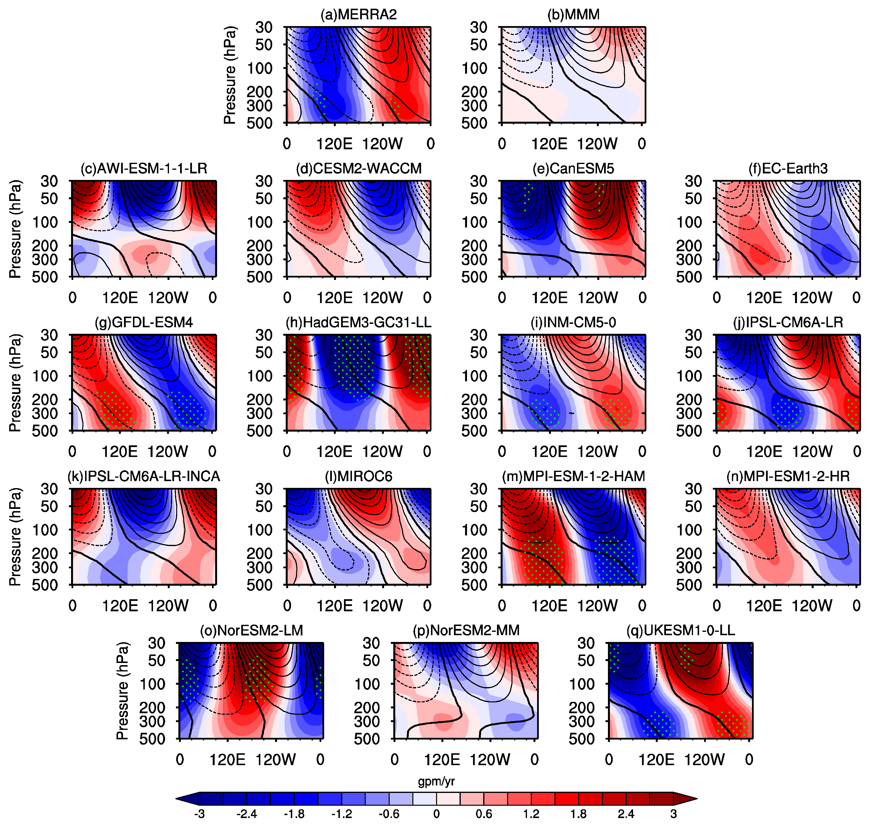
Figure 10 shows the height-longitude cross-section along 60° N of zonal wavenumber-1 geopotential height tendency in February for the period 1981–2014 and the climatological mean of zonal wavenumber-1 geopotential height in the same month. The climatological mean for MERRA2 displays a baroclinic structure and tilts westward with increasing height. Furthermore, the zonal wavenumber-1 geopotential height tendency is in-phase with the climatological mean wavenumber-1 geopotential height, suggesting an amplification of wavenumber-1 baroclinic waves and their strong upward propagation into the stratosphere in the high latitudes of the Northern Hemisphere. Propagation of wavenumber-1 planetary waves into the stratosphere could push the Arctic vortex to move toward the Eurasian continent and promotes vortex displacement events [20,21,67]. Although the multi-model mean cannot reproduce the enhancement in baroclinic waves associated with wavenumber one component after 1980, CanESM5, IPSL-CM6A-LR, and UKESM1-0-LL models can well capture the baroclinic structure shown in MERRA2, making them capture the shift of polar vortex towards Eurasia (Figure 8d,k,r and Figure 9b). Simulations of AWI-ESM-1-1-LR, HadGEM3-GC31-LL, and NorESM2-MM display a similar structure to the multi-model mean, which shows a more eastward shift of the polar vortex towards eastern Siberia compared with MERRA2 (Figure 8c,h,q). Results of CESM2-WACCM, EC-Earth3, GFDL-ESM4, IPSL-CM6A-LR-INCA, MPI-ESM-1-2-HAM, and MPI-ESM1-2-HR indicate that the zonal wavenumber-1 geopotential height tendency mostly is out-of-phase with the climatological mean. In summary, the shift of the polar vortex towards the Eurasian continent during late winter is associated with enhanced zonal wavenumber-1 geopotential height. This result indicates that a realistic simulation of zonal wavenumber-1 by CMIP6 models is the prerequisite for a reasonable simulation of the polar vortex shift.
4. Discussion
In this study, we compare MERRA2 and ERA-I reanalysis data with CMIP6 models and evaluate the simulation performance of CMIP6 on the Arctic stratospheric polar vortex. It can be found that there are some inconsistencies between MERRA2 and ERA-I datasets (Table 2), which may be due to the potential impacts of reanalysis data systems and the uncertainty of reanalysis data. It is worthwhile to compare reanalysis data with the observations and to explore reasons for these inconsistencies in the future. In addition, previous studies have shown that the high-top model is better than the low-top model in characterizing stratospheric processes [30,33]. However, we investigated the relationship between the polar vortex intensity biases and the model top (Figure 3b), and found that there is no significant difference in polar vortex intensity between high-top and low-top models, which may be because the model top has little influence on polar vortex intensity in the lower stratosphere. The ability of the high-top and low-top models to capture the characteristics of the stratospheric polar vortex in the middle and upper stratosphere deserves further investigation. Moreover, previous studies suggested that compared with the WACCM-SC without chemical–climate coupling, the simulation by the CESM1-WACCM model with interactive chemistry shows a smaller bias against realistic stratospheric processes [39]. Similarly, Zhang et al. [68] the study shows that the coupled chemical–radiative–dynamical processes play a key role in the CMIP6 simulation of the stratospheric processes. Kawa et al. [69] pointed out a possible feedback process between ozone chemistry and the dynamics of the Arctic stratospheric polar vortex. Therefore, further studies are needed to clarify how the chemical processes, particularly those related to ozone, in the CMIP6 model affect the variability of the polar vortex.
5. Conclusions
The polar vortex is one of the key components in the stratosphere–troposphere coupling system. The present study evaluates the ability of 16 CMIP6 models for the simulation of long-term change and interannual variability of the Arctic stratospheric polar vortex during winter. We also analyzed the relationship between the biases in the strength and position of the polar vortex and the biases in planetary waves across different models. Based on a comparison with the MERRA2 dataset, it is found that the 16 CMIP6 models generally can reproduce the features of the polar vortex identified in MERRA2, although the polar vortex shape in the multi-model mean is more circular than that in MERRA2 (Figure 1). The models reproduce the climatological mean shape and edge of the polar vortex (Figure 2b). Most of the 16 CMIP6 models yield negative PV biases within the polar vortex (Figure 2c–r), indicating that the modeled polar vortex is weaker than that shown in MERRA2. An interesting feature is that the correlation between the area bias and the strength bias of the simulated polar vortex is negative (Figure 3a). In addition, most CMIP6 models reproduce the spatial pattern of the polar vortex with spatial correlation coefficients greater than 0.85 in each wintertime month and greater than 0.9 in DJF mean (Figure 4).
The present study analyzed the daily climatology of zonal mean westerlies during winter (Figure 5). The multi-model mean can capture the zonal mean westerlies increase through early winter and its maximum value in mid-winter. However, the occurrence time of the maximum wind in the multi-model mean lags behind that in MERRA2 (Figure 5b). Compared with MERRA2, positive biases in zonal mean westerlies in late winter and negative biases in early winter are found in simulations of AWI-ESM-1-1-LR, CESM2-WACCM, HadGEM3-GC31-LL, INM-CM5-0, MIROC6, and MPI-ESM-1-2-HAM. In addition, this study analyzed the long-term trend in zonal mean westerlies during winter (Figure 6). The multi-model mean well displays the negative trend of zonal wind during middle and late winter, although the trend magnitude is relatively weaker. Note that AWI-ESM-1-1-LR, CanESM5, GFDL-ESM4, HadGEM3-GC31-LL, and IPSL-CM5A2-INCA can well simulate a significant negative trend of zonal mean westerlies in late winter, which is consistent with the trend shown in MERRA2. Furthermore, this study highlights that an increase in convergence of EP flux by zonal wavenumber one accumulated in early winter corresponds to a stronger deceleration of zonal mean westerlies in late winter (Figure 7). All CMIP6 models underestimate the accumulation of EP flux in the stratosphere.
Few studies have evaluated the performance of CMIP6 models in simulating the long-term change of the stratospheric polar vortex position since 1980. In this study, the multi-model mean shows a non-significant increase in the fractional area of the polar vortex over Eurasia and a non-significant decline over North America (Figure 9b,c). CanESM5, IPSL-CM5A2-INCA, IPSL-CM6A-LR, and UKESM1-0-LL reproduce the positive trend of PV over the Eurasian continent (Figure 9b,c) and the increase in upward propagation of baroclinic waves into the stratosphere (Figure 10), both of which are shown in MERRA2. This suggests that the model’s ability to accurately simulate the propagation of planetary waves with wavenumber one is a key factor in simulating the shift of the stratospheric polar vortex. The analysis further reveals that model biases in lower-stratospheric polar vortex strength and shape in the lower stratosphere are independent of the model top height (Figure 3b).
Author Contributions
Conceptualization, J.Z.; methodology, S.Z. and J.Z.; software, S.Z.; validation, S.Z., C.Z. and M.X.; formal analysis, S.Z., J.Z. and C.Z.; investigation, S.Z., J.Z. and C.Z.; data curation, S.Z., C.Z. and Z.W.; writing—original draft preparation, S.Z., J.Z., C.Z., M.X., J.K., Z.W. and X.X.; visualization, S.Z. and X.X.; supervision, J.Z., C.Z., M.X. and J.K.; project administration, J.Z.; funding acquisition, J.Z.; writing—review & editing, S.Z., J.Z. and M.X. All authors have read and agreed to the published version of the manuscript.
Funding
This research was sponsored by the National Natural Science Foundation of China (Jiankai Zhang, 42075062 and Wenshou Tian, 42130601), the Fundamental Research Funds for the Central Universities (Jiankai Zhang, lzujbky-2021-ey04). The Met Office CSSP-China Programme provides funding support for the POzSUM project (James Keeble).
Data Availability Statement
The ERA-I dataset applied in this work are available at https://apps.ecmwf.int/datasets/data/interim-full-daily/levtype=sfc/ (accessed on 1 December 2020). The MERRA2 data are obtained from https://disc.gsfc.nasa.gov/datasets/M2I3NPASM_5.12.4/summary?keywords=%22MERRA-2%22 (accessed on 1 December 2020). The CMIP6 models can be downloaded from https://esgf-node.llnl.gov/search/cmip6/ (accessed on 1 December 2020).
Acknowledgments
We thank the scientific teams at the European Centre for Medium-Range Weather Forecasts (ECMWF) for providing ERA-I reanalysis data. We also thank the scientific teams at National Aeronautics and Space Administration (NASA) for providing the MERRA-2 reanalysis data. We acknowledge the World Climate Research Programme to coordinate and promote CMIP6 through its Working Group on Coupled Modelling. We thank various climate modelling groups for producing and making available their model outputs. We appreciate the Earth System Grid Federation (ESGF) for archiving the data and providing public access and the multiple funding agencies that support CMIP6 and ESGF.
Conflicts of Interest
The authors declare no conflict of interest.
References
- Waugh, D.W.; Polvani, L.M. Stratospheric polar vortices, in The Stratosphere: Dynamics, Transport, and Chemistry. Geophys. Monogr. Ser. 2010, 190, 43–57. [Google Scholar]
- Waugh, D.W.; Sobel, A.H.; Polvani, L.M. What Is the Polar Vortex and How Does It Influence Weather? Bull. Am. Meteorol. Soc. 2017, 98, 37–44. [Google Scholar] [CrossRef]
- Ambaum, M.H.P.; Hoskins, B. The NAO troposphere-stratosphere connection. J. Clim. 2002, 15, 1969–1978. [Google Scholar] [CrossRef]
- Mitchell, D.M.; Gray, L.J.; Anstey, J.; Baldwin, M.P.; Charlton-Perez, A.J. The influence of stratospheric vortex displacements and splits on surface climate. J. Clim. 2013, 26, 2668–2682. [Google Scholar] [CrossRef]
- Seviour, W.J.M.; Mitchell, D.M.; Gray, L.J. A practical method to identify displaced and split stratospheric polar vortex events. Geophys. Res. Lett. 2013, 40, 5268–5273. [Google Scholar] [CrossRef]
- O’Callaghan, A.; Joshi, M.; Stevens, D.; Mitchell, D. The effects of different sudden stratospheric warming types on the ocean. Geophys. Res. Lett. 2014, 41, 7739–7745. [Google Scholar] [CrossRef]
- Baldwin, M.P.; Dunkerton, T.J. Stratospheric harbingers of anomalous weather regimes. Science 2001, 294, 581–584. [Google Scholar] [CrossRef]
- Kim, B.M.; Son, S.-W.; Min, S.K.; Jeong, J.H.; Kim, S.J.; Zhang, X.; Shim, T.; Yoon, J.H. Weakening of the stratospheric polar vortex by Arctic sea-ice loss. Nat. Commun. 2014, 5, 4646. [Google Scholar] [CrossRef]
- Cohen, J.; Screen, J.; Furtado, J.; Barlow, M.; Whittleston, D.; Coumou, D.; Francis, J.; Dethloff, K.; Entekhabi, D.; Overland, J.; et al. Recent Arctic amplification and extreme mid-latitude weather. Nat. Geosci. 2014, 7, 627–637. [Google Scholar] [CrossRef]
- White, I.P.; Garfinkel, C.I.; Cohen, J.; Jucker, M.; Rao, J. The impact of split and displacement sudden stratospheric warmings on the troposphere. J. Geophys. Res. Atmos. 2021, 126, e2020JD033989. [Google Scholar] [CrossRef]
- Zhang, R.; Tian, W.; Zhang, J.; Huang, J.; Xie, F.; Xu, M. The corresponding tropospheric environments during downward-extending and non-downward-extending events of stratospheric Northern Annular Mode anomalies. J. Clim. 2019, 32, 1857–1873. [Google Scholar] [CrossRef]
- Huang, J.; Tian, W.; Zhang, J.; Huang, Q.; Tian, H.; Luo, J. The connection between extreme stratospheric polar vortex events and tropospheric blockings. Q. J. R. Meteorol. Soc. 2017, 143, 1148–1164. [Google Scholar] [CrossRef]
- Hu, J.; Li, T.; Xu, H. Relationship between the North Pacific Gyre Oscillation and the onset of stratospheric final warming in the northern Hemisphere. Clim. Dyn. 2018, 51, 3061–3075. [Google Scholar] [CrossRef]
- Hu, D.; Guan, Z.; Liu, M.; Wang, T. Is the relationship between stratospheric Arctic vortex and Arctic Oscillation steady? J. Geophys. Res. Atmos. 2021, 126, e2021JD035759. [Google Scholar] [CrossRef]
- Limpasuvan, V.; Thompson, D.W.J.; Hartmann, D.L. The life cycle of the Northern Hemisphere sudden stratospheric warmings. J. Clim. 2004, 17, 2584–2596. [Google Scholar] [CrossRef]
- Kolstad, E.W.; Breiteig, T.; Scaife, A.A. The association between stratospheric weak polar vortex events and cold air outbreaks in the Northern Hemisphere. Q. J. R. Meteorol. Soc. 2010, 136, 886–893. [Google Scholar] [CrossRef]
- Huang, J.; Tian, W. Eurasian cold air outbreaks under different Arctic stratospheric polar vortex strengths. J. Atmos. Sci. 2019, 76, 1245–1264. [Google Scholar] [CrossRef]
- Xie, J.; Hu, J.; Xu, H.; Liu, S.; He, H. Dynamic Diagnosis of Stratospheric Sudden Warming Event in the Boreal Winter of 2018 and Its Possible Impact on Weather over North America. Atmosphere 2020, 11, 438. [Google Scholar] [CrossRef]
- Rao, J.; Garfinkel, C.I.; White, I.P. Impact of the Quasi-Biennial Oscillation on the Northern Winter Stratospheric Polar Vortex in CMIP5/6 Models. J. Clim. 2020, 33, 4787–4813. [Google Scholar] [CrossRef]
- Zhang, J.; Tian, W.; Chipperfield, M.P.; Xie, F.; Huang, J. Persistent shift of the Arctic polar vortex towards the Eurasian continent in recent decades. Nat. Clim. Chang. 2016, 6, 1094–1099. [Google Scholar] [CrossRef]
- Huang, J.; Tian, W.; Gray, L.J.; Zhang, J.; Li, Y.; Luo, J.; Tian, H. Preconditioning of Arctic stratospheric polar vortex shift events. J. Clim. 2018, 31, 5417–5436. [Google Scholar] [CrossRef]
- Waugh, D.W.; Randel, W.J. Climatology of Arctic and Antarctic polar vortices using elliptical diagnostics. J. Atmos. Sci. 1999, 56, 1594–1613. [Google Scholar] [CrossRef]
- Polvani, L.M.; Waugh, D.W. Upward wave activity flux as a precursor to extreme stratospheric events and subsequent anomalous surface weather regimes. J. Clim. 2004, 17, 3548–3554. [Google Scholar] [CrossRef]
- Gerber, E.P.; Polvani, L.M. Stratosphere–troposphere coupling in a relatively simple AGCM: The importance of stratospheric variability. J. Clim. 2009, 22, 1920–1933. [Google Scholar] [CrossRef]
- Castanheira, J.M.; Liberato, M.L.R.; de la Torre, L.; Graf, H.-F.; DaCamara, C.C. Baroclinic Rossby Wave Forcing and Barotropic Rossby Wave Response to Stratospheric Vortex Variability. J. Atmos. Sci. 2009, 66, 902–914. [Google Scholar] [CrossRef]
- McKenna, C.M.; Bracegirdle, T.J.; Shuckburgh, E.F.; Haynes, P.H.; Joshi, M.M. Arctic sea ice loss in different regions leads to contrasting Northern Hemisphere impacts. Geophys. Res. Lett. 2018, 45, 945–954. [Google Scholar] [CrossRef]
- Hu, Y.; Tung, K.K.; Liu, J. A closer comparison of early and late-winter atmospheric trends in the Northern Hemisphere. J. Clim. 2005, 18, 3204–3216. [Google Scholar] [CrossRef]
- Garfinkel, C.I.; Son, S.-W.; Song, K.; Aquila, V.; Oman, L.D. Stratospheric variability contributed to and sustained the recent hiatus in Eurasian winter warming. Geophys. Res. Lett. 2017, 44, 374–382. [Google Scholar] [CrossRef]
- Hu, D.; Guan, Z.; Tian, W.; Ren, R. Recent strengthening of the stratospheric Arctic vortex response to warming in the central North Pacific. Nat. Commun. 2018, 9, 1697. [Google Scholar] [CrossRef]
- Hurwitz, M.M.; Calvo, N.; Garfinkel, C.I.; Butler, A.H.; Ineson, S.; Cagnazzo, C.; Manzini, E.; Peña-Ortiz, C. Extra-tropical atmospheric response to ENSO in the CMIP5 models. Clim. Dyn. 2014, 43, 3367–3376. [Google Scholar] [CrossRef]
- Rao, J.; Garfinkel, C.I.; Wu, T.; Lu, Y.; Chu, M. Mean State of the Northern Hemisphere Stratospheric Polar Vortex in Three Generations of CMIP Models. J. Clim. 2022, 35, 4603–4625. [Google Scholar] [CrossRef]
- Elsbury, D.; Peings, Y.; Magnusdottir, G. CMIP6 models underestimate the Holton-Tan effect. Geophys. Res. Lett. 2021, 48, e2021GL094083. [Google Scholar] [CrossRef]
- Gong, H.; Wang, L.; Chen, W.; Wu, R.; Zhou, W.; Liu, L.; Nath, D.; Lan, X. Diversity of the Wintertime Arctic Oscillation Pattern among CMIP5 Models: Role of the Stratospheric Polar Vortex. J. Clim. 2019, 32, 5235–5250. [Google Scholar] [CrossRef]
- Charlton-Perez, A.J.; Baldwin, M.P.; Birner, T.; Black, R.X.; Butler, A.H.; Calvo, N.; Davis, N.A.; Gerber, E.P.; Gillett, N.; Hardiman, S.; et al. On the lack of stratospheric dynamical variability in low-top versions of the CMIP5 models. J. Geophys. Res. Atmos. 2013, 118, 2494–2505. [Google Scholar] [CrossRef]
- Haase, S.; Matthes, K.; Latif, M.; Omrani, N. The Importance of a Properly Represented Stratosphere for Northern Hemisphere Surface Variability in the Atmosphere and the Ocean. J. Clim. 2018, 31, 8481–8497. [Google Scholar] [CrossRef]
- Kim, J.; Son, S.-W.; Gerber, E.P.; Park, H. Defining Sudden Stratospheric Warming in Climate Models: Accounting for Biases in Model Climatologies. J. Clim. 2017, 30, 5529–5546. [Google Scholar] [CrossRef]
- Wu, Z.; Reichler, T. Variations in the Frequency of Stratospheric Sudden Warmings in CMIP5 and CMIP6 and Possible Causes. J. Clim. 2020, 33, 10305–10320. [Google Scholar] [CrossRef]
- Hall, R.J.; Mitchell, D.M.; Seviour, W.J.M.; Wright, C.J. Persistent model biases in the CMIP6 representation of stratospheric polar vortex variability. J. Geophys. Res. Atmos. 2021, 126, e2021JD034759. [Google Scholar] [CrossRef]
- Oehrlein, J.; Chiodo, G.; Polvani, L.M. The effect of interactive ozone chemistry on weak and strong stratospheric polar vortex events. Atmos. Chem. Phys. 2020, 20, 10531–10544. [Google Scholar] [CrossRef]
- Eyring, V.; Bony, S.; Meehl, G.A.; Senior, C.A.; Stevens, B.; Stouffer, R.J.; Taylor, K.E. Overview of the Coupled Model Intercomparison Project Phase 6 (CMIP6) experimental design and organization. Geosci. Model Dev. 2015, 9, 1937–1958. [Google Scholar] [CrossRef]
- Gelaro, R.; McCarty, W.; Suárez, M.J.; Todling, R.; Molod, A.; Takacs, L.; Randles, C.A.; Darmenov, A.; Bosilovich, M.G.; Reichle, R.; et al. The Modern-Era Retrospective Analysis for Research and Applications, version 2 (MERRA-2). J. Clim. 2017, 30, 5419–5454. [Google Scholar] [CrossRef]
- Dee, D.P.; Uppala, S.M.; Simmons, A.J.; Berrisford, P.; Poli, P.; Kobayashi, S.; Andrae, U.; Balmaseda, M.A.; Balsamo, G.; Bauer, P.; et al. The ERA-Interim reanalysis: Configuration and performance of the data assimilation system. Q. J. R. Meteorol. Soc. 2011, 137, 553–597. [Google Scholar] [CrossRef]
- Checa-Garcia, R.; Hegglin, M.I.; Kinnison, D.; Plummer, D.A.; Shine, K.P. Historical tropospheric and stratospheric ozone radiative forcing using the CMIP6 database. Geophys. Res. Lett. 2018, 45, 3264–3273. [Google Scholar] [CrossRef]
- Danek, C.; Shi, X.; Stepanek, C.; Yang, H.; Barbi, D.; Hegewald, J.; Lohmann, G. AWI AWI-ESM1.1LR Model Output Prepared for CMIP6 CMIP Historical. Version 20201101. Earth System Grid Federation. 2020. Available online: wdc-climate.de (accessed on 1 June 2022).
- Swart, N.C.; Cole, J.N.S.; Kharin, V.V.; Lazare, M.; Scinocca, J.F.; Gillett, N.P.; Anstey, J.; Arora, V.; Christian, J.R.; Jiao, Y.; et al. CCCma CanESM5 Model Output Prepared for CMIP6 CMIP Historical. Version 20190429. Earth System Grid Federation. 2020. Available online: wdc-climate.de (accessed on 1 June 2022).
- Danabasoglu, G. NCAR CESM2-WACCM Model Output Prepared for CMIP6 CMIP Historical. Version 20201101. Earth System Grid Federation. 2019. Available online: wdc-climate.de (accessed on 1 June 2022).
- EC-Earth Consortium (EC-Earth). EC-Earth-Consortium EC-Earth3 Model Output Prepared for CMIP6 CMIP Historical. Version 20190711. Earth System Grid Federation. 2019. Available online: wdc-climate.de (accessed on 1 June 2022).
- Krasting, J.P.; John, J.G.; Blanton, C.; McHugh, C.; Nikonov, S.; Radhakrishnan, A.; Rand, K.; Zadeh, N.T.; Balaji, V.; Durachta, J.; et al. NOAA-GFDL GFDL-ESM4 Model Output Prepared for CMIP6 CMIP Historical. Version 20201101. Earth System Grid Federation. 2018. Available online: wdc-climate.de (accessed on 1 June 2022).
- Ridley, J.; Menary, M.; Kuhlbrodt, T.; Andrews, M.; Andrews, T. MOHC HadGEM3-GC31-LL Model Output Prepared for CMIP6 CMIP. Version 20201101. Earth System Grid Federation. 2018. Available online: wdc-climate.de (accessed on 1 June 2022).
- Volodin, E.; Mortikov, E.; Gritsun, A.; Lykossov, V.; Galin, V.; Diansky, N.; Gusev, A.; Kostrykin, S.; Iakovlev, N.; Shestakova, A.; et al. INM INM-CM5-0 Model Output Prepared for CMIP6 CMIP Historical. Version 20201101. Earth System Grid Federation. 2019. Available online: wdc-climate.de (accessed on 1 June 2022).
- Boucher, O.; Denvil, S.; Levavasseur, G.; Cozic, A.; Caubel, A.; Foujols, M.; Meurdesoif, Y.; Balkanski, Y.; Checa-Garcia, R.; Hauglustaine, D.; et al. IPSL IPSL-CM5A2-INCA Model Output Prepared for CMIP6 CMIP Historical. Version 20201101. Earth System Grid Federation. 2020. Available online: wdc-climate.de (accessed on 1 June 2022).
- Boucher, O.; Denvil, S.; Caubel, A.; Foujols, M.A. IPSL IPSL-CM6A-LR Model Output Prepared for CMIP6 CMIP Historical. Version 20201101. Earth System Grid Federation. Available online: wdc-climate.de (accessed on 1 June 2022).
- Boucher, O.; Denvil, S.; Levavasseur, G.; Cozic, A.; Caubel, A.; Foujols, M.-A.; Meurdesoif, Y.; Balkanski, Y.; Checa-Garcia, R.; Hauglustaine, D.; et al. IPSL IPSL-CM6A-LR-INCA Model Output Prepared for CMIP6 CMIP Historical. Version 20201101. Earth System Grid Federation. 2021. Available online: wdc-climate.de (accessed on 1 June 2022).
- Tatebe, H.; Watanabe, M. MIROC MIROC6 Model Output Prepared for CMIP6 CMIP Historical. Version 20201101. Earth System Grid Federation. 2018. Available online: wdc-climate.de (accessed on 1 June 2022).
- Neubauer, D.; Ferrachat, S.; Siegenthaler-Le Drian, C.; Stoll, J.; Folini, D.S.; Tegen, I.; Wieners, K.-H.; Mauritsen, T.; Stemmler, I.; Barthel, S.; et al. HAMMOZ-Consortium MPI-ESM1.2-HAM Model Output Prepared for CMIP6 CMIP Historical. Version 20201101. Earth System Grid Federation. 2019. Available online: wdc-climate.de (accessed on 1 June 2022).
- Jungclaus, J.; Bittner, M.; Wieners, K.-H.; Wachsmann, F.; Schupfner, M.; Legutke, S.; Giorgetta, M.; Reick, C.; Gayler, V.; Haak, H.; et al. MPI-M MPI-ESM1.2-HR Model Output Prepared for CMIP6 CMIP Historical. Version 20201101. Earth System Grid Federation. 2019. Available online: wdc-climate.de (accessed on 1 June 2022).
- Seland, Ø.; Bentsen, M.; Oliviè, D.J.L.; Toniazzo, T.; Gjermundsen, A.; Graff, L.S.; Debernard, J.B.; Gupta, A.K.; He, Y.; Kirkevåg, A.; et al. NCC NorESM2-LM Model Output Prepared for CMIP6 CMIP Historical. Version 20201101. Earth System Grid Federation. 2019. Available online: wdc-climate.de (accessed on 1 June 2022).
- Bentsen, M.; Oliviè, D.J.L.; Seland, O.; Toniazzo, T.; Gjermundsen, A.; Graff, L.S.; Debernard, J.B.; Gupta, A.K.; He, Y.; Kirkevåg, A.; et al. NCC NorESM2-MM Model Output Prepared for CMIP6 CMIP Historical. Version 20201101. Earth System Grid Federation. 2019. Available online: wdc-climate.de (accessed on 1 June 2022).
- Tang, Y.; Rumbold, S.; Ellis, R.; Kelley, D.; Mulcahy, J.; Sellar, A.; Walton, J.; Jones, C. MOHC UKESM1.0-LL Model Output Prepared for CMIP6 CMIP Historical. Version 20201101. Earth System Grid Federation. 2019. Available online: wdc-climate.de (accessed on 1 June 2022).
- Nash, E.R.; Newman, P.A.; Rosenfield, J.E.; Schoeberl, M.R. An objective determination of the polar vortex using Ertel’s potential vorticity. J. Geophys. Res. Atmos. 1996, 101, 9471–9478. [Google Scholar] [CrossRef]
- Zhang, J.; Xie, F.; Ma, Z.; Zhang, C.; Xu, M.; Wang, T.; Zhang, R. Seasonal evolution of the quasi-biennial oscillation impact on the Northern Hemisphere polar vortex in winter. J. Geophys. Res. Atmos. 2019, 124, 12568–12586. [Google Scholar] [CrossRef]
- Andrews, D.G.; Holton, J.R.; Leovy, C.B. Middle Atmosphere Dynamics; Academic Press: San Diego, CA, USA, 1987; p. 128. [Google Scholar]
- Taylor, K.E. Summarizing multiple aspects of model performance in a single diagram. J. Geophys. Res. Atmos. 2001, 106, 7183–7192. [Google Scholar] [CrossRef]
- Ralf, J.; Klaus, D.; Dörthe, H. Stratospheric response to Arctic sea ice retreat and associated planetary wave propagation changes. Tellus A Dyn. Meteorol. Oceanogr. 2013, 65, 19375. [Google Scholar]
- Chen, W.; Yang, S.; Huang, R. Relationship between stationary planetary wave activity and the East Asian winter monsoon. J. Geophys. Res. Atmos. 2005, 110, D14110. [Google Scholar] [CrossRef]
- Seviour, W.J.M. Weakening and shift of the Arctic stratospheric polar vortex: Internal variability or forced response? Geophys. Res. Lett. 2017, 44, 3365–3373. [Google Scholar] [CrossRef]
- Mitchell, D.M.; Charlton-Perez, A.J.; Gray, L.J. Characterizing the variability and extremes of the stratospheric polar vortices using 2D moment analysis. J. Atmos. Sci. 2011, 68, 1194–1213. [Google Scholar] [CrossRef]
- Zhang, K.; Duan, J.; Zhao, S.; Zhang, J.; Keeble, J.; Liu, H. Evaluating the ozone valley over the Tibetan Plateau in CMIP6 models. Adv. Atmos. Sci. 2022, 39, 1167–1183. [Google Scholar] [CrossRef]
- Kawa, S.R.; Bevilacqua, R.M.; Margitan, J.J.; Douglass, A.R.; Schoeberl, M.R.; Hoppel, K.W.; Sen, B. Interaction between dynamics and chemistry of ozone in the setup phase of the Northern Hemisphere polar vortex. J. Geophys. Res. Atmos. 2002, 107, 8310. [Google Scholar] [CrossRef]
Figure 1.
(a) Edge (contour lines) and center (shaped dots) of climatological polar vortex averaged over the isentropic levels between 430–600 K during December–January–February (DJF) for the period 1980/81–2013/14 based on ERA-Interim, MERRA2, simulations of 16 CMIP6 models and multi-model mean. (b) Same as (a) except that it is presented as a Mercator projection.

Figure 2.
December–January–February (DJF) mean PV (unit: 1 PVU, 1 PVU = 10−6 m2 s−1 K kg−1) averaged over the isentropic levels between 430–600 K for the period 1980/81–2013/14 based on (a) MERRA2, (b) multi-model mean. (c–r) PV differences between individual CMIP6 model simulations and MERRA2. The green solid line represents the corresponding polar vortex edge in MERRA2 and/or CMIP6 model simulation.

Figure 3.
(a) Correlation between bias in polar vortex area and bias in polar vortex strength based on MERRA2 and 16 CMIP6 models for the period 1980/81–2013/14. (b) Ranking of polar vortex strength bias versus model top height of the 16 CMIP6 models. The ‘prob’ denotes the statistical significance according to Student’s t-test.
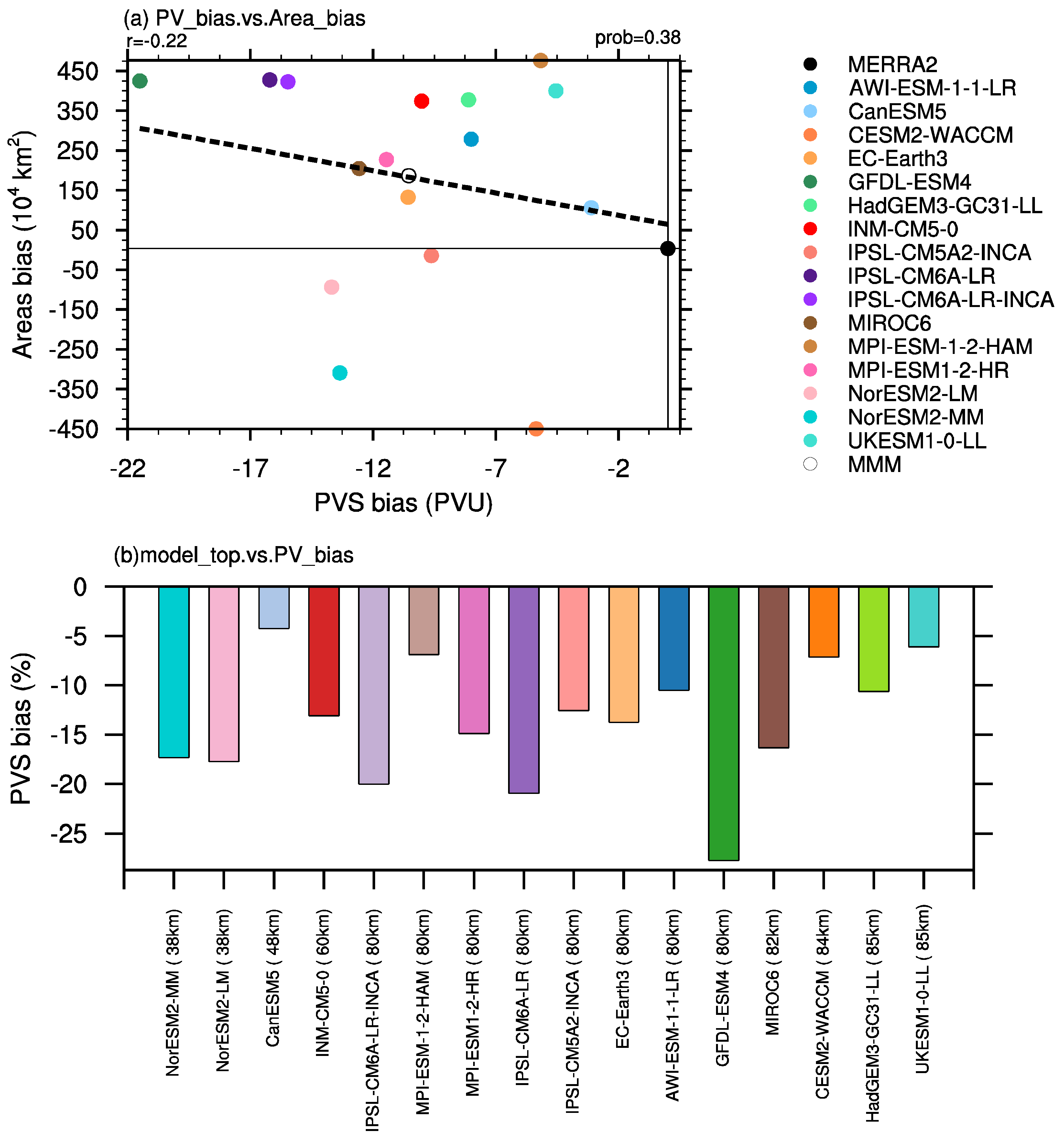
Figure 4.
Taylor diagram for climatological mean of PV simulated by 16 CMIP6 models. These simulations are compared with MERRA2 over polar cap (60°–90°N). All data are averaged over the isentropic levels between 430–600 K for the period of 1980/81–2013/14 in each winter month (a–c) and for DJF mean (d). In Taylor diagram, the angular axis shows spatial correlation between simulated and observed climatology of PV, the radial axis shows spatial SD normalized against that of the MERRA2, “REF” represents the reference line. More details can be found in Taylor (2001) [63]. Different symbols denote different percentage biases between MERRA2 and model simulations. Each symbol represents an individual CMIP6 model.

Figure 5.
Time evolution of climatological mean of daily zonal mean zonal wind (units: m/s) over the levels between 1–300 hPa in the polar cap (60°–90° N) during winter derived from (a) MERRA2, (b) multi-model mean for the period of 1980/81–2013/14. (c–r) Differences in climatological mean of zonal wind between individual CMIP6 model simulations and MERRA2 (D01 means 01, December; J10 means 10, January; F19 means 19, February).

Figure 6.
The trend of daily zonal mean zonal wind over the levels between 1–300 hPa in the polar cap (60°–90° N) for the period 1980/81-2013/14 derived from (a) MERRA2, (b) multi-model mean and (c–r) each CMIP6 model simulation. Green dotted regions are for values statistically significant at the 90% confidence level by Student’s t-test.
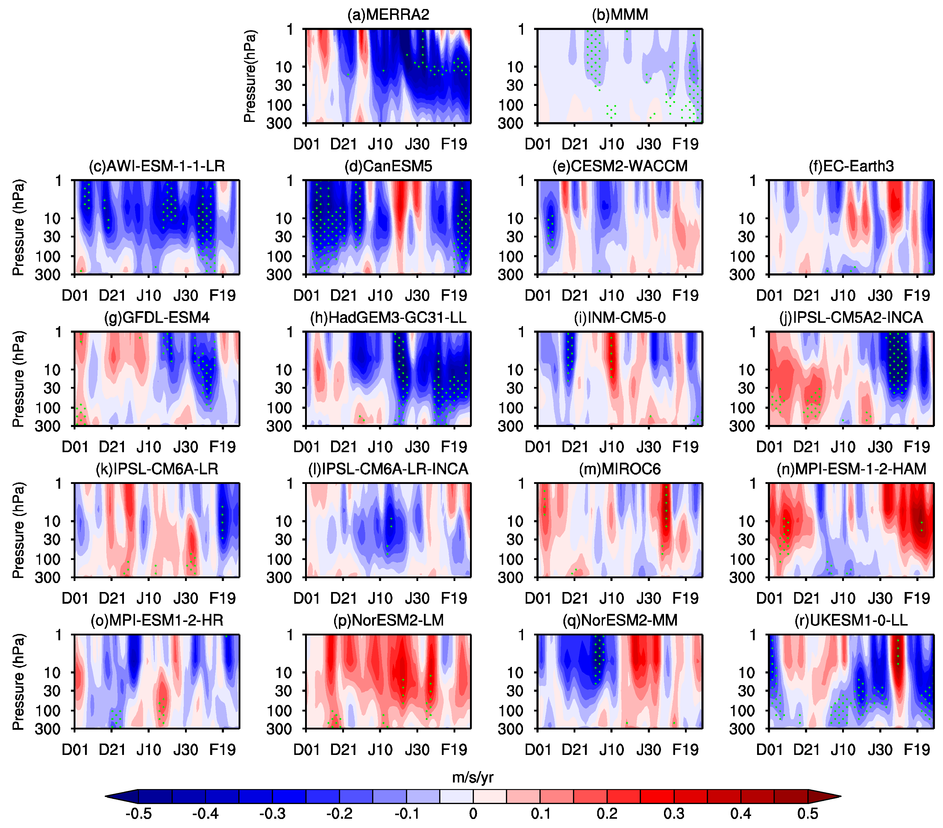
Figure 7.
Correlation between the trend of EP-flux divergence in zonal wavenumber-1 accumulated in early winter from 10 December to 10 January at 1–10 hPa averaged over 45°–75° N and the trend in zonal mean zonal winds averaged at 1–100 hPa over 60°–90° N in the late winter from 10 January to 28 February for the period 1980/81–2013/14. All calculations are based on daily mean derived from MERRA2 and simulations of 16 CMIP6 models. Each symbol represents an individual CMIP6 model, while the black dot denotes MERRA2.
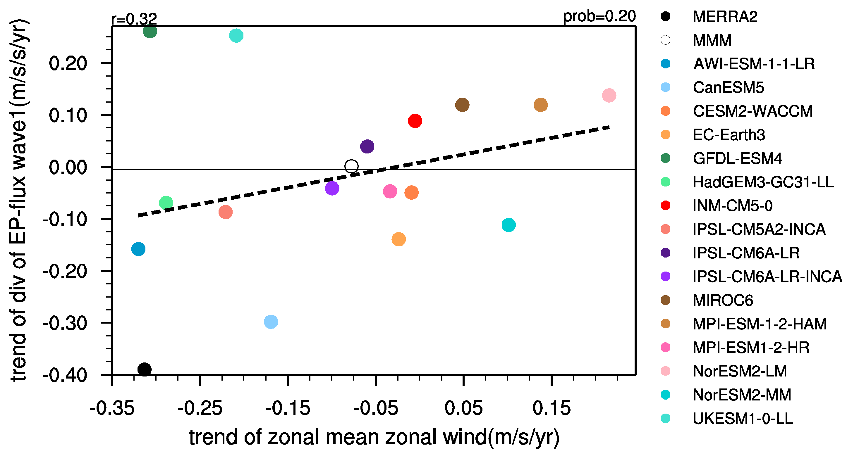
Figure 8.
Climatological mean of polar vortex edge (purple contour) and linear trend of PV averaged between 430–600 K (shaded) for the period 1981–2014 in February derived from (a) MERRA2, (b) multi-model mean and (c–r) each CMIP6 model.
Figure 8.
Climatological mean of polar vortex edge (purple contour) and linear trend of PV averaged between 430–600 K (shaded) for the period 1981–2014 in February derived from (a) MERRA2, (b) multi-model mean and (c–r) each CMIP6 model.

Figure 9.
(a) Spatial correlation coefficient of PV trend over isentropic levels within 430–600 K in the Northern Hemisphere (30°–90° N) between individual CMIP6 model simulations and MERRA2 for the period of 1981–2014 in February. Linear trends of fractional area over (b) Eurasian continent and (c) North America for the period of 1981–2014 based on MERRA2 and individual CMIP6 model simulations. The fractional area over a specific region (e.g., Eurasian or North American) is defined as the area of polar vortex in the region divided by the total area of the polar vortex. This definition is the same as that defined in Figure 1c of Zhang et al. [20]. The solid columns represent the corresponding linear trends that are statistically significant at the 90% confidence levels, whereas the dotted columns indicate trends that are not significant at the 90% confidence level. Each color column represents an individual CMIP6 model, while the black column denotes MERRA2.
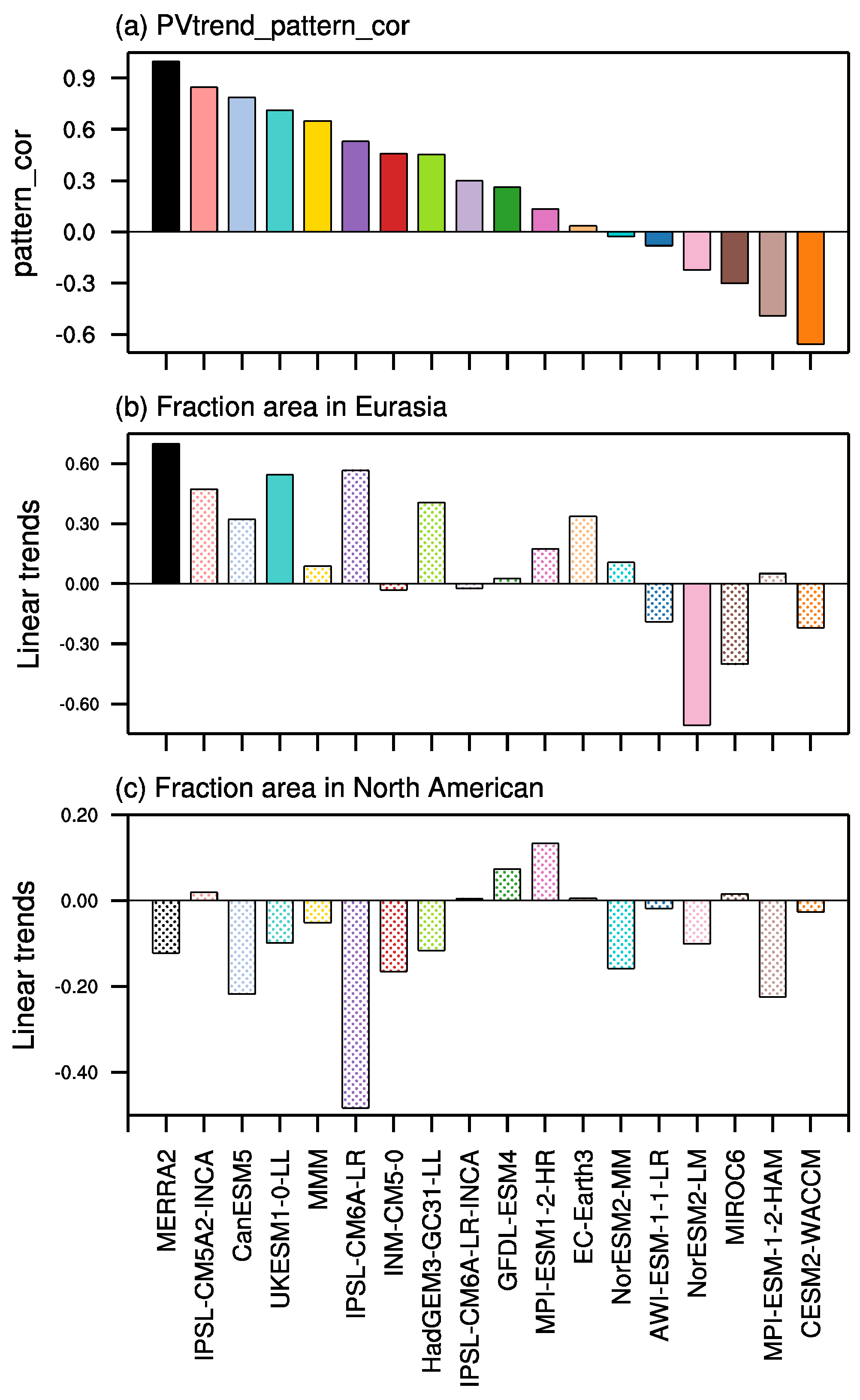
Figure 10.
Height-longitude cross sections along 60° N of zonal wave-1 geopotential height trend over the period 1981–2014 (shaded areas). Black contours indicate climatological mean of zonal wave-1 geopotential height along 60° N for the period 1981–2014 in February derived from (a) MERRA2, (b) multi-model mean and (c–q) individual CMIP6 model simulations. Green dotted regions are for values statistically significant at the 90% confidence level by Student’s t-test.

Table 1.
Description of models and data available at the time when this work was being performed in 2021. Major information includes model names and their horizontal and vertical resolutions, the stratospheric chemistry scheme used, the simulations produced by each model, and the Earth System Grid Federation (ESGF) reference for the model datasets. Options of the stratospheric chemistry scheme include interactive chemistry schemes (fully coupled complex chemistry schemes), simplified online schemes (simple, linear schemes) and prescribed stratospheric ozone field. Different models may use different schemes. Most models that run with prescribed stratospheric ozone use the CMIP6 dataset [43] except CESM2 and NorESM2, which use prescribed ozone data simulated by CESM2-WACCM. The meteorological variables used in the present study include temperature, horizontal winds, and geopotential height. Note that the geopotential height of IPSL-CM5A2-INCA is not available in this study.
| Model | Resolution | Stratospheric Chemistry | The Meteorological Fields | Datasets |
|---|---|---|---|---|
| AWI-ESM-1-1-LR | 192 × 96 longitude–latitude; 47 levels; top level 80 km | Prescribed (CMIP6 dataset) | Historical | Danek et al. [44] |
| CanESM5 | 128 × 64 longitude–latitude; 49 levels; top level 1 hPa | Prescribed (other) | Historical | Swart et al. [45] |
| CESM-WACCM | 288 × 96 longitude–latitude; 70 levels; top level 4.5 × 10⁻⁶ hPa | Interactive chemistry | Historical | Danabasoglu [46] |
| EC-Earth3 | 512 × 256 longitude–latitude; 91 levels; top level 0.01 hPa | Prescribed (CMIP6 dataset) | Historical | EC-Earth Consortium [47] |
| GFDL-ESM4 | 360 × 180 longitude–latitude; 49 levels; top level 0.01 hPa | Interactive chemistry | Historical | Krasting et al. [48] |
| HadGEM3-GC31-LL | 192 × 144 longitude/latitude; 85 levels; top level 85 km | Prescribed (CMIP6 dataset) | Historical | Ridley et al. [49] |
| INM-CM5-0 | 180 × 120 longitude/latitude; 73 levels; top level sigma = 0.0002 (~0.2 hPa) | Prescribed (CMIP6 dataset) | Historical | Volodin et al. [50] |
| IPSL-CM5A2-INCA | 96 × 96 longitude/latitude; 39 levels; top level 80 km | Interactive chemistry | Historical | Boucher et al. [51] |
| IPSL-CM6A-LR | 144 × 143 longitude–latitude; 79 levels; top level 80 km | Prescribed (CMIP6 dataset) | Historical | Boucher et al. [52] |
| IPSL-CM6A-LR-INCA | 144 × 143 longitude/latitude; 79 levels; top level 80 km | Prescribed (CMIP6 dataset) | Historical | Boucher et al. [53] |
| MIROC6 | 256 × 128 longitude/latitude; 81 levels; top level 0.004 hPa | Prescribed (CMIP6 dataset) | Historical | Tatebe et al. [54] |
| MPI-ESM-1-2-HAM | 192 × 96 longitude–latitude; 47 levels; top level 0.01 hPa | Interactive chemistry | Historical | Neubauer et al. [55] |
| MPI-ESM1-2-HR | 384 × 192 longitude–latitude; 95 levels; top level 0.01 hPa | Prescribed (CMIP6 dataset) | Historical | Jungclaus et al. [56] |
| NorESM2-LM | 144 × 96 longitude–latitude; 32 levels; top level 3 hPa | Prescribed (other) | Historical | Seland et al. [57] |
| NorESM2-MM | 288 × 192 longitude–latitude; 32 levels; top level 3 hPa | Prescribed (other) | Historical | Bentsen et al. [58] |
| UKESM1-0-LL | 192 × 144 longitude–latitude; 85 levels; top level 85 km | Interactive chemistry | Historical | Tang et al. [59] |
Table 2.
Center position, strength and size of the polar vortex from two reanalysis datasets and model simulations, and biases of the polar vortex strength and area in various model simulations compared with Reanalysis (the averaged between ERA-I and MERRA2), ERA-I and MERRA2.
Table 2.
Center position, strength and size of the polar vortex from two reanalysis datasets and model simulations, and biases of the polar vortex strength and area in various model simulations compared with Reanalysis (the averaged between ERA-I and MERRA2), ERA-I and MERRA2.
| Model | PV Center | Areas (104 km2) | Area Bias (%) (vs. ERA-I) | Area Bias (%) (vs. MERRA2) | The Polar Vortex Strength | The Bias of Polar Vortex Strength (%) (vs. ERA-I) | The Bias of Polar Vortex Strength (%) (vs. MERRA2) |
|---|---|---|---|---|---|---|---|
| ERA-I | (80.37°N, 31.77°E) | 2085.79 | 0 | −2.60 | 78.7 | 0 | 0.56 |
| MERRA2 | (80.44°N, 32.25°E) | 2141.54 | 2.67 | 0 | 78.2 | −0.56 | 0 |
| AWI-ESM-1-1-LR | (82.76°N, 33.08°E) | 2416.54 | 15.86 | 12.84 | 70.2 | −10.75 | −10.25 |
| CanESM5 | (80.65°N, 34.56°E) | 2244.16 | 7.59 | 4.79 | 75.1 | −4.53 | −4.00 |
| CESM-WACCM | (80.23°N, 36.39°E) | 1688.08 | −19.07 | −21.17 | 72.9 | −7.38 | −6.87 |
| EC-Earth3 | (82.23°N, 24.10°E) | 2270.43 | 8.85 | 6.02 | 67.6 | −14.02 | −13.54 |
| GFDL-ESM4 | (83.18°N, 10.33°E) | 2562.83 | 22.87 | 19.67 | 56.7 | −27.92 | −27.51 |
| HadGEM3-GC31–LL | (81.18°N, 41.30°E) | 2515.47 | 20.60 | 17.46 | 70.1 | −10.89 | −10.39 |
| INM-CM5-0 | (84.06°N, 28.38°E) | 2512.17 | 20.44 | 17.31 | 68.2 | −13.32 | −12.83 |
| IPSL-CM5A2-INCA | (82.51°N, 5.44°E) | 2123.78 | 1.82 | −0.83 | 68.6 | −12.82 | −12.33 |
| IPSL-CM6A-LR | (80.53°N, 5.51°E) | 2565.55 | 23.00 | 19.80 | 62.0 | −21.19 | −20.75 |
| IPSL-CM6A-LR-INCA | (81.61°N, 4.31°E) | 2560.84 | 22.78 | 19.58 | 62.7 | −20.24 | −19.80 |
| MIROC6 | (82.22°N, 14.94°E) | 2342.82 | 12.32 | 9.40 | 65.6 | −16.56 | −16.09 |
| MPI-ESM-1-2-HAM | (82.90°N, 31.61°E) | 2614.31 | 25.34 | 22.08 | 73.0 | −7.15 | −6.63 |
| MPI-ESM1-2-HR | (80.18°N, 32.04°E) | 2365.23 | 13.40 | 10.45 | 66.8 | −15.14 | −14.67 |
| NorESM2-LM | (78.58°N, 43.81°E) | 2044.62 | −1.97 | −4.53 | 64.5 | −17.98 | −17.52 |
| NorESM2-MM | (78.43°N, 29.12°E) | 1829.03 | −12.31 | −14.59 | 64.9 | −17.56 | −17.10 |
| UKESM1-0-LL | (81.76°N, 36.10°E) | 2538.13 | 21.69 | 18.52 | 73.7 | −6.36 | −5.84 |
| Multi-model mean | (82.26°N, 26.83°E) | 2324.62 | 11.45 | 8.55 | 67.7 | −13.99 | −13.51 |
Publisher’s Note: MDPI stays neutral with regard to jurisdictional claims in published maps and institutional affiliations. |
© 2022 by the authors. Licensee MDPI, Basel, Switzerland. This article is an open access article distributed under the terms and conditions of the Creative Commons Attribution (CC BY) license (https://creativecommons.org/licenses/by/4.0/).
Share and Cite
MDPI and ACS Style
Zhao, S.; Zhang, J.; Zhang, C.; Xu, M.; Keeble, J.; Wang, Z.; Xia, X. Evaluating Long-Term Variability of the Arctic Stratospheric Polar Vortex Simulated by CMIP6 Models. Remote Sens. 2022, 14, 4701. https://doi.org/10.3390/rs14194701
AMA Style
Zhao S, Zhang J, Zhang C, Xu M, Keeble J, Wang Z, Xia X. Evaluating Long-Term Variability of the Arctic Stratospheric Polar Vortex Simulated by CMIP6 Models. Remote Sensing. 2022; 14(19):4701. https://doi.org/10.3390/rs14194701
Chicago/Turabian StyleZhao, Siyi, Jiankai Zhang, Chongyang Zhang, Mian Xu, James Keeble, Zhe Wang, and Xufan Xia. 2022. "Evaluating Long-Term Variability of the Arctic Stratospheric Polar Vortex Simulated by CMIP6 Models" Remote Sensing 14, no. 19: 4701. https://doi.org/10.3390/rs14194701
Note that from the first issue of 2016, this journal uses article numbers instead of page numbers. See further details here.