Technical Note

Analysis of the Atmospheric Duct Existence Factors in Tropical Cyclones Based on the SHAP Interpretation of Extreme Gradient Boosting Predictions

The College of Meteorology and Oceanology, National University of Defense Technology, Changsha 410073, China
*
Author to whom correspondence should be addressed.
Remote Sens. 2022, 14(16), 3952; https://doi.org/10.3390/rs14163952
Submission received: 25 June 2022 / Revised: 9 August 2022 / Accepted: 11 August 2022 / Published: 14 August 2022

Abstract

:
The atmospheric duct (AD) is an anomalous structure in which electromagnetic waves can make transhorizon propagation. ADs often occur in the formation, development and disappearance of tropical cyclones (TCs). In this work, the eXtreme Gradient Boosting (XGBoost) model is used to predict TC ducts and a relatively high accuracy of 81.3% is obtained. Shapely additional explanations (SHAP) values of the features including TC parameters and local meteorological parameters are employed to interpret XGBoost model predictions of the TC ducts existence. Furthermore, the importance ranking of the features is revealed, among which the distance between dropsondes and TC eyes is the most important. In addition, the detailed relationships between the AD existence and the features are presented. Hence, this work can not only improve the knowledge of the relationship between TC ducts and the features, but also be of great value to the ducts prediction.

1. Introduction

The propagation of the electromagnetic wave (EMW) in the atmosphere depends on the atmospheric refraction index. The atmospheric duct (AD) is an anomalous refraction structure. When the AD appears, the propagation path of EMW bends downward and the energy will be restricted in the AD layer with small dissipation. Hence, the propagation length of the EMW can be extremely long. As a result, the detectability of radars and the smoothness of the communication system improve greatly. On the other hand, the existence of the ducting layer results in the radar electromagnetic blind area and positioning errors.
The formation of the AD is associated with many synoptic processes. In 2004, Von Engeln et al. [1] held the opinion that elevated ducts are usually caused by the subsidence of air masses and the diurnal warming and cooling of the planetary boundary layer (PBL). Sun et al. [2] found the elevated ducts were caused by the intermittent turbulence in the PBL for the first time in 2016. Turton et al. [3] enumerated five synoptic processes in favor of the formation of ducts in their work in 1988. In recent years, some research focused on the atmospheric ducts related to the tropical cyclones (TCs). Pan et al. pointed out that the atmospheric condition in the western and northwestern edge of the TCs was beneficial to the formation of ADs [4]. The ducts induced by TCs over the northwestern Pacific Ocean were analyzed based on the Global Position System (GPS) dropsonde data by Ding et al. [5]. They found that the ducts formed in the transition zones tended to be stronger and thicker than those formed inside the TCs. In 2019, Shi et al. [6] researched the impact of the typhoon on the evaporation duct in the Northwestern Pacific Ocean and discovered that the evaporation duct height in the typhoon eye was very low primarily due to the low wind speed in this region. Fei et al. [7] investigated the impacts of the Bogus Data Assimilation (BDA) and sea spray parameterization (SSP) on the typhoon ducts prediction induced by Typhoon Mindule (2004) and GPS dropsonde data is used to compare with the predictions. They found that the probability of the existence of typhoon ducts is nearly equal in every direction around the typhoon center and most of them are elevated ducts. However, the sample size of their research is relatively small and only one typhoon with ducts is investigated. As a result, the conclusion they obtained may be one-sided.
In recent years, reanalysis data have been widely utilized to perform surface, elevated and evaporation duct climatology [8,9]. Based on these works, many statistical characteristics of ducts were obtained. However, because of its coarse vertical resolution, the ducting layers in high layers could not be reflected. Therefore, the data from GPS dropsondes, aircraft and radiosondes were used in the literature. Manjula et al. analyzed the diurnal variation of atmospheric ducts in different seasons and the ducts characteristics contrast between different seasons in Gadanki [10]. Zhao et al. [11] used radiosonde data on the balloons by ship to detect the ducts occurrence in 2013, and they concluded that the probability of ducts in the South China Sea is about 75% during 2010–2012. However, the shortcomings of these works are obvious. Firstly, the sample number is small, which makes the conclusions lack universality. Secondly, traditional dropsondes data have a vertical resolution of about 100 m, failing to detect thin ducting layers [12,13].
Nowadays, as machine learning becomes more and more popular, it has been applied to the field of meteorology much more frequently [14,15,16,17,18,19,20]. This method is suitable for big data analysis and can easily establish the mapping relationship between the features and the targets. For the atmospheric duct, many machine learning algorithms are also used to improve the prediction accuracy. Zhu et al. [21] proposed a method based on a multilayer perceptron to predict the evaporation duct height (EDH) and improves the accuracy a lot compared with the Paulus–Jeske (P-J) model. Han et al. [22] put forward a method for EDH nowcasting based on a long short-term memory (LSTM) network and a fully connected network. It turns out that this method has a higher accuracy than traditional time series forecasting methods. Extreme gradient boosting (XGBoost) is a popular machine learning algorithm based on the decision tree [23]. It is much faster than traditional machine learning algorithms. In addition, it has had a very good prediction performance in many research works in recent years [24,25].
In this work, the high-vertical-resolution, long-term GPS dropsonde data from the National Oceanic and Atmospheric Administration (NOAA), SRTM15 elevation data from the National Aeronautics and Space Administration (NASA) and the National Bureau of Image and Mapping (NIMA), TC-related information from the International Best Track Archive for Climate Stewardship (IBTrACS) project from NOAA and ERA-5 reanalysis dataset from European Centre for Medium-Range Weather Forecasts (ECWMF) are used to analyze the TC ducts existence factors to the western and eastern coast of America from 1996 to 2020 based on XGBoost. Furthermore, the SHAP (shapely additional explanations) values [26] are applied to interpret the XGBoost predictions of TC ducts existence to find out how different factors influence the ducts existence.

2. Data, Model and Methods

2.1. The Method of Determining TC Ducts

The definition of the radio refractivity was put forward in 1953 [27]; the expression is as follows:
N = 77.6 p T 5.6 e T + 3.75 × 10 5 e T 2
where T is the absolute temperature (Kelvin), p is the atmospheric pressure (hPa), e is the water vapor pressure (hPa). After taking the earth curvature into consideration, the modified refractivity is introduced:
M = N + z R × 10 6 = N + 0.157 z
where R is the radius of the earth with a value of 6.371 × 10 6 meters, and z is the height above the sea surface (meters). The occurrence of the AD is judged by d M / d z < 0 as the curvature radius of the EMW track is smaller than that of the earth in this case; thus, the EMW is trapped in the specific layer and the AD is formed. Temperature, pressure and humidity profiles from GPS dropsondes are used to calculate the profiles of the modified refractivity. Since some of the dropsondes positions are on land, the elevation change is taken into account.
Due to the existence of turbulence and instrumental noise, the raw data is firstly processed by the software named Atmospheric Sounding Processing Environment (ASPEN) from the National Center for Atmospheric Research (NCAR) (http://www.eol.ucar.edu/software/aspen (accessed on 13 June 2022)). This software can analyze the data, perform smoothing, sensor time response corrections and remove suspect data points [28]. After the profiles are calculated, each potential ducting layer corresponds to a cut-off wavelength, which represents the ability to capture the EMW. The longer it is, the more stable the ducting layer will be. The cut-off wavelength is calculated by the equation below [29]:
λ max = 2 × C × d × δ M 3
where λ max is the cut-off wavelength (meters), d is the depth of the ducting layer (meters), and δ M is the duct strength (M). C is a constant value of 5.66 × 10 3 for an elevated duct and 3.773 × 10 3 for a surface duct. In this work, the potential ducting layers whose λ max 0.5 are considered as effective ducting layers. The reason for taking this index as a restriction is the two characteristics of the duct are taken into consideration. A layer that satisfies the above equations can be regarded as an atmospheric duct when both of the duct strength and the duct thickness are big enough. In this way, the unreal ducts caused by the instrumental error and the random disturbance error can be filtered since their thicknesses are too small or their strength is too tiny. With the above steps, the negative effects are eliminated and the real ducting layers are obtained. Finally, 15,216 profiles are calculated in 164 TCs from 1996 to 2020 (Figure 1).

2.2. Datasets for the Predictions of TC Ducts

The temperature, pressure and humidity data come from the GPS dropsondes deployed from high altitudes by hurricane research aircraft from NOAA from 1996 to 2020 for over 20,000 times (https://www.aoml.noaa.gov/hrd/data_sub/dropsonde.html (accessed on 13 June 2022)). The data including temperature, humidity, wind speed and direction are available every 0.5 s. The vertical resolution of the data is about 5–15 m. Secondly, the elevation data used here is SRTM15 Digital Elevation Model (DEM) from the NASA and the NIMA. The horizontal resolution of the data is 450 m, and the coverage area is global land. With the computed elevation and other parameters combined, the profile of modified refractivity can be calculated.
The TC-related information in this paper is from the IBTrACS project version 04 published by NOAA (ncdc.noaa.gov/ibtracs/index.php (accessed on 13 June 2022)) [30]. The variables have a temporal resolution of 3 h for each TC. According to the prior knowledge and reasonable conjecture, four variables are chosen to be the features: TC grades (TC intensities are classified into eleven categories of unknown type, post-tropical, misc-disturbances, subtropical, tropical-depression and tropical-storm from −5 to 0 and categories 1–5 by the Saffir–Simpson scale based on the 10 min average maximum sustained winds), TC radius of the maximum winds (RMW), the distance between dropsondes and the TC eye (TC-dropsonde distance) and the positional relation between dropsondes and TC tracks (The dropsonde can be on the four quadrants: the left-front, left-back, right-front and right-back side of TC tracks, respectively, represented by 1–4). We call it the dropsonde quadrant. Among the points in the tracks of the TC, the variables at the point whose time is closest to the deploying time are selected to be the features of the profile.
Furthermore, meteorological parameters at standard pressure levels used in this paper are derived from the ERA-5 reanalysis dataset (https://cds.climate.copernicus.eu/cdsapp#!/home (accessed on 13 June 2022)) from ECWMF. The temporal resolution of the dataset is one hour and the spatial resolution is 0.25° × 0.25°. The maximum height we consider does not exceed 5000 m since most ADs occur below this height [31]. As a result, the pressure levels include 1000 hPa, 975 hPa, 950 hPa, 925 hPa, 900 hPa, 875 hPa, 850 hPa, 825 hPa, 800 hPa, 775 hPa, 750 hPa, 700 hPa, 650 hPa, 600 hPa, 550 hPa and 500 hPa. For better summary in the following text, these pressure levels are divided into three parts: upper layer (500–600 hPa), middle layer (600–750 hPa) and lower layer (775–1000 hPa) according to the pressure-altitude correspondence. The parameters are the specific humidity, the temperature and zonal and meridional winds at these levels. In terms of the selection of grid data, according to Peng and Shu [32], the horizontal advection range of the dropsondes can be negligible compared to the hurricane scale in most cases, and since the maximum height is 5000 m, the horizontal range within the height does not exceed a few kilometers. Based on the above analysis, we conclude that GPS dropsondes maintain a relatively fixed position, that is, dropsondes can detect local vertical meteorological parameters precisely. Hence, the grid in which the dropsonde is located is chosen and the time is chosen to be the hourly time closest to the deploying time of the dropsonde. The local meteorological parameters combined with the TC parameters and the locations of dropsondes make up the feature set, and then predict the TC ducts (Table 1).

2.3. XGBoost Model

XGBoost is converted from the gradient boosting decision tree (GBDT) algorithm, which avoids over-fitting by adding regular terms into the cost function [33,34]. Its basic theory is as follows [25]:
y ^ i ( t ) = k = 1 t f k ( x i ) = y ^ i ( t 1 ) + f t ( x i )
where t is the number of basic tree models, f t ( x i ) is the prediction of the t-th tree for the i-th sample and y ^ i ( t ) is the prediction of the t basic tree models for the i-th sample.
The goal of the algorithm is to make the integrated model achieve the best performance, which also means minimizing the loss function:
ξ = i n l ( y i , y ^ i ) + k = 1 t Ω ( f k ) Ω ( f t ) = γ T + 1 2 λ j = 1 T w j 2
where l is a twice differentiable convex function used to measure the error between the actual value y ^ and the predicted value y ^ i . T is the number of nodes in a decision tree and w j is the weight of the j -th node in all leaf nodes. γ and λ is the difficulty of node segmentation and the regularization coefficient, respectively. Ω ( f ) is the summary of the complexity of the t trees which can be used for the penalty function.
Since XGBoost uses the forward iteration, the t-th tree is focused on and the predictions of the former t 1 trees can be regarded as constant:
ξ ( t ) = i n l ( y i , y ^ i ) + k = 1 t Ω ( f k ) = i = 1 n l ( y i , y ^ i ( t 1 ) + f t ( x i ) ) + k = 1 t Ω ( f k ) = i = 1 n l ( y i , y ^ i ( t 1 ) + f t ( x i ) ) + Ω ( f t ) + C
Next, Taylor series expansion is utilized for the loss function, and the original loss function is modified as:
ξ ( t ) = i = 1 n [ l ( y i , y ^ i ( t 1 ) ) + g i f t ( x i ) + 1 2 h i f t 2 ( x i ) ] + Ω ( f t ) + C
where g i represents the first derivative and h i represents the second derivative. Then, Equation (5) is plugged into Equation (7):
ξ ( t ) = j = 1 T [ G j w j + 1 2 ( H j + λ ) w j 2 ] + γ T G j = i I j g i H j = i I j h i
To obtain w j , the loss function is taken the derivative of with regard to it. Then, w j and ξ can be expressed as below:
w j = G j H j + λ ξ = 1 2 j = 1 T G j 2 H j + λ + γ T
XGBoost classifier includes the following parameters: learning_rate (control the learning speed), max_depth (the max depth of the decision tree), n_estimators (maximum number of decision trees), min_child_weight (defines the minimum sum of weights required in a child), reg_lambda (L2 regularization term), reg_alpha (L1 regularization term), subsample (control the proportion of random sampling number), colsample_bytree (control the proportion of random sampling features) and gamma (minimum decrease in the loss function for node splitting).
As for the data features and labels, the features we use are as described in the previous section. These features are employed to predict the occurrence of TC ducts. We use 0 and 1 as labels. The 1 represents no TC ducts in this profile, and the 0 represents the opposite. The sampling method used in this work is over-sampling due to the large gap between the numbers of data of the two classes. Specifically, the dataset includes 5727 samples with the value of 0 and 9489 samples with the value of 1. Artificial points are added to the samples with value 1 randomly, making the number of the two classes equal-sized.
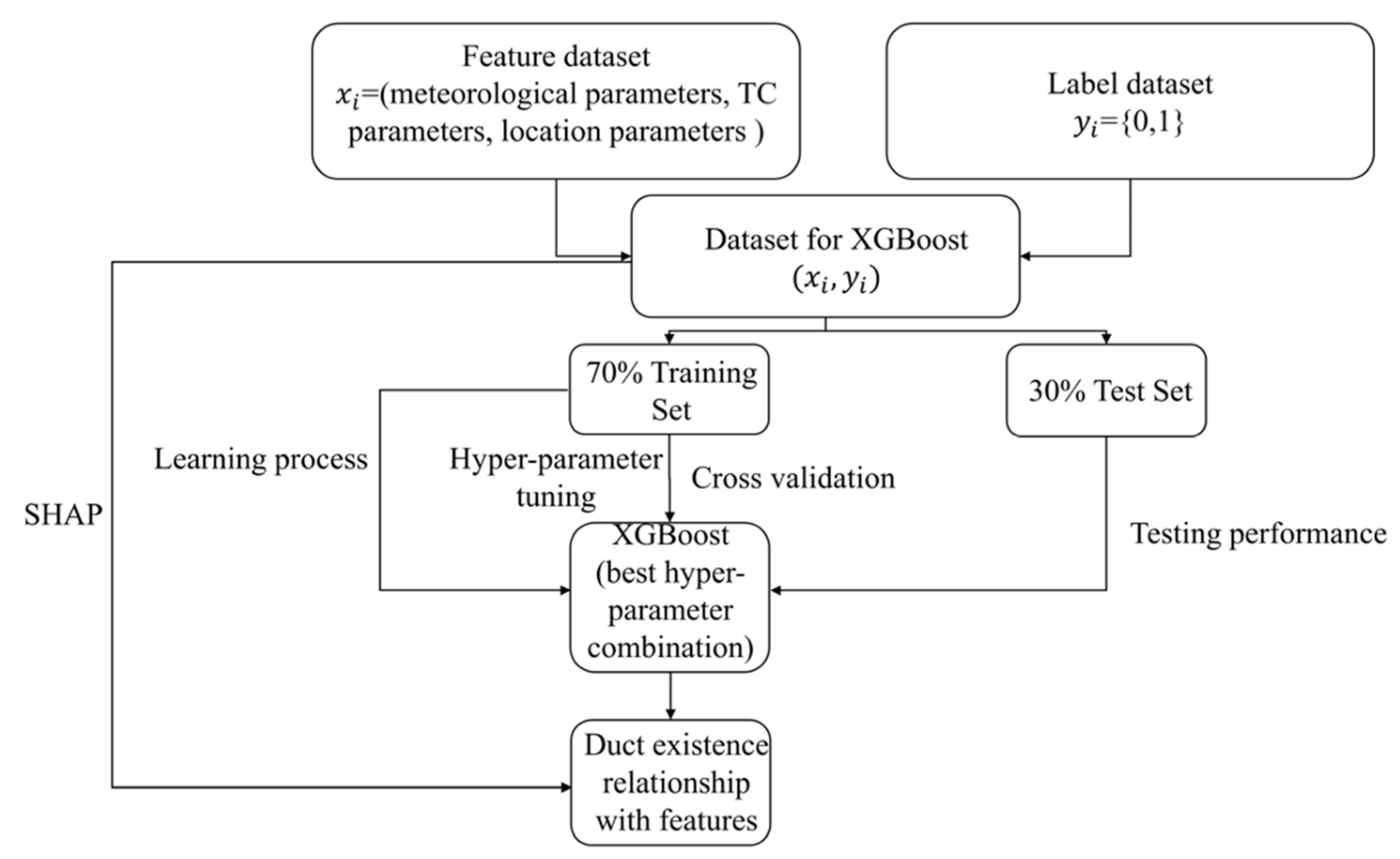
Next, the total data set is divided into a training set (70% of the sample size) and a testing set (30% of the sample size). The loss function is chosen to be binary cross entropy. Every parameter is set within a fixed range according to prior knowledge. The grid search algorithm is used to find all the parameter combinations within the range of settings and then the performance of each combination is calculated utilizing cross-validation on the training set [35]. After a large number of computer experiments are accomplished, the best parameter combination is obtained as is shown in Table 2.
The estimation indexes are chosen to be the kappa index and classification accuracy. Kappa index is a measure of agreement between measured data and simulated data [36]. It is a popular indicator in the present field of machine learning, especially in the field of spatial matching. The expression of Kappa index is as follows:
κ = p 0 p e 1 p e p e = a 1 × b 1 + a 2 × b 2 n × n
where p 0 is the sum of the correctly classified samples for each category divided by the total number of samples, a 1 , a 2 represent the real number of samples for each category and b 1 , b 2 represent the predicted number of samples for each category. The relationship between its values and the degree of agreement is as follows [37]:
strong   agreement high   agreement moderate   agreement poor   agreement κ > 0.8 0.6 < κ < 0.8 0.4 < κ < 0.6 κ < 0.4

2.4. SHAP Interpretation for the TC Ducts Prediction

SHAP is a “model interpretation” package developed in Python that interprets the output of any machine learning model. SHAP can quantitatively analyze the relationships between machine learning algorithm predictions and input variables. The SHAP value for each variable represents its effects and importance on the predictions. SHAP values can sort the importance of the variables to the predictions, and thus, SHAP can be used for feature selection. Furthermore, compared with the original XGBoost ranking, SHAP has two big advantages, consistency and accuracy, respectively. As for consistency, it means that when the number of features changes, the change of the original feature importance ranking order will be as little as possible. With regard to the accuracy, this advantage makes sure that each feature’s contribution to the total importance remains the same when some of the features are deleted from the feature set [26,38]. The basic theory of the SHAP is called the shapely value method put forward by Shapely [39] in 1953. It belongs to the field of the cooperative game to solve the contradiction caused by the distribution of interests in the process of cooperation. One advantage of applying the Shapely value is that the benefits are distributed according to the marginal contribution rate of members to the alliance, that is, the benefits shared by member i are equal to the average value of marginal benefits created by the member for the alliance he participates in. The basic theory is as follows:
φ i ( v ) = S N [ ( S 1 ) ! ( n S ) ! ] n ! × [ v ( S ) v ( S \ { i } ) ]
where n is the number of members in the cooperative game system, and N = { 1 , 2 , , n } . S is the subset of N composed of different members. v ( S ) represents the benefits of the alliance S and φ i ( v ) represents the benefits obtained by member i of the alliance S . S represents the number of members in the alliance S . n ! represents the n factorial. S \ { i } represents the set after the element i is removed from S . The marginal contribution created by member i participating in different alliances S is denoted as [ v ( S ) v ( S \ { i } ) ] . The weight of the benefits created by the member i in the whole alliance is denoted as [ ( S 1 ) ! ( n S ) ! ] n ! .
The basic theory of the shapely value method is applied to SHAP. In machine learning, every feature in the feature set is a member of the alliance. There is a predicted value of the machine learning algorithm for each sample, and the SHAP value is the value assigned to each feature in the feature set. The formula for SHAP value is as follows:
z i = z b a s e + h ( x i 1 ) + h ( x i 2 ) + + h ( x i j )
where x i j represents the j-th feature of the i-th sample, and z i represents the predicted value of the i-th sample. z b a s e is the baseline of the model and h ( x i j ) means the value contributed to the final prediction by the j-th feature of the i-th sample.
In this work, this method is employed to find the relationship between the existence of TC ducts and different factors. Furthermore, the importance of the factors is sorted to find out the primary factor. Additionally, the primary cause of each TC duct can be discovered.
In summary, the feature set including meteorological parameters, TC parameters and location parameters, combined with the label set is used in XGBoost algorithm to predict the existence of the AD in oceanic TC. Then, the SHAP is utilized to interpret the predictions of the XGBoost and analyze the relations between the TC-AD and these features. The overall structure of the algorithm is shown in Figure 2.

3. Results and Discussion

3.1. The Performance of the XGBoost Algorithm on the Testing Dataset

The trained model is tested by kappa index and accuracy on the testing set, which can reach 0.6258 and 81.30%, respectively. From Equation (11), our features have a high agreement with the TC ducts existence. Logistic regression is a generalized linear regression analysis model and belongs to supervised learning. The derivation process and calculation method are similar to the regression method. Nevertheless, it is mainly used to address dichotomies problems. It is used here as the benchmark model to compare its performance with that of XGBoost. Logistic regression has the following parameters: regularization parameter (C), penalty term (penalty), optimization method (solver) and the best parameters combination are C = 0.1, penalty = L2 and solver = ”lbfgs”. The testing accuracy of the model is about 69.5% and the testing kappa index is about 0.391. It turns out that the XGBoost model performance improves a lot compared with logistic regression.

3.2. The Top 20 Most Important Features to the Existence of the AD

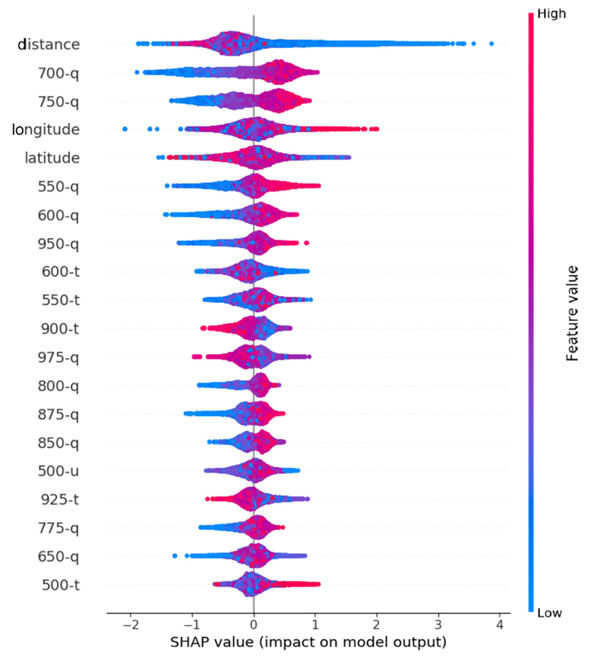
SHAP is used to quantitatively analyze the predictions of the XGBoost model trained on the training set, and then the importance of features is sorted according to the SHAP values on the total dataset (Figure 3). This figure presents the SHAP values of the top 20 most important features and how they affect the predictions. The positive values indicate the probability of TC ducts becoming lower and the negative indicates the opposite. The gradient color from red to blue on the color bar corresponds to the feature values from high to low. As shown in Figure 3, Firstly, the horizontal distance between the TC eye and the dropsonde has the greatest effect on the TC ducts existence. however, the relationship between them is not linear. Secondly, the geographical position of the dropsonde takes the second position among the TC parameters. With regard to the TC grades, the RMW of TCs and the relative position of dropsondes to TCs, they have few effects on the existence. From the aspect of local meteorological parameters of dropsondes, the humidity at the pressure level of 700 hPa is the most crucial factor. Additionally, it was found that the humidity at various levels is the most important, the temperature at levels comes second. As for the zonal and meridional wind at levels, the only level worthy of attention is the 500 hPa pressure level.

3.3. The Relationship between AD Existence and the Features

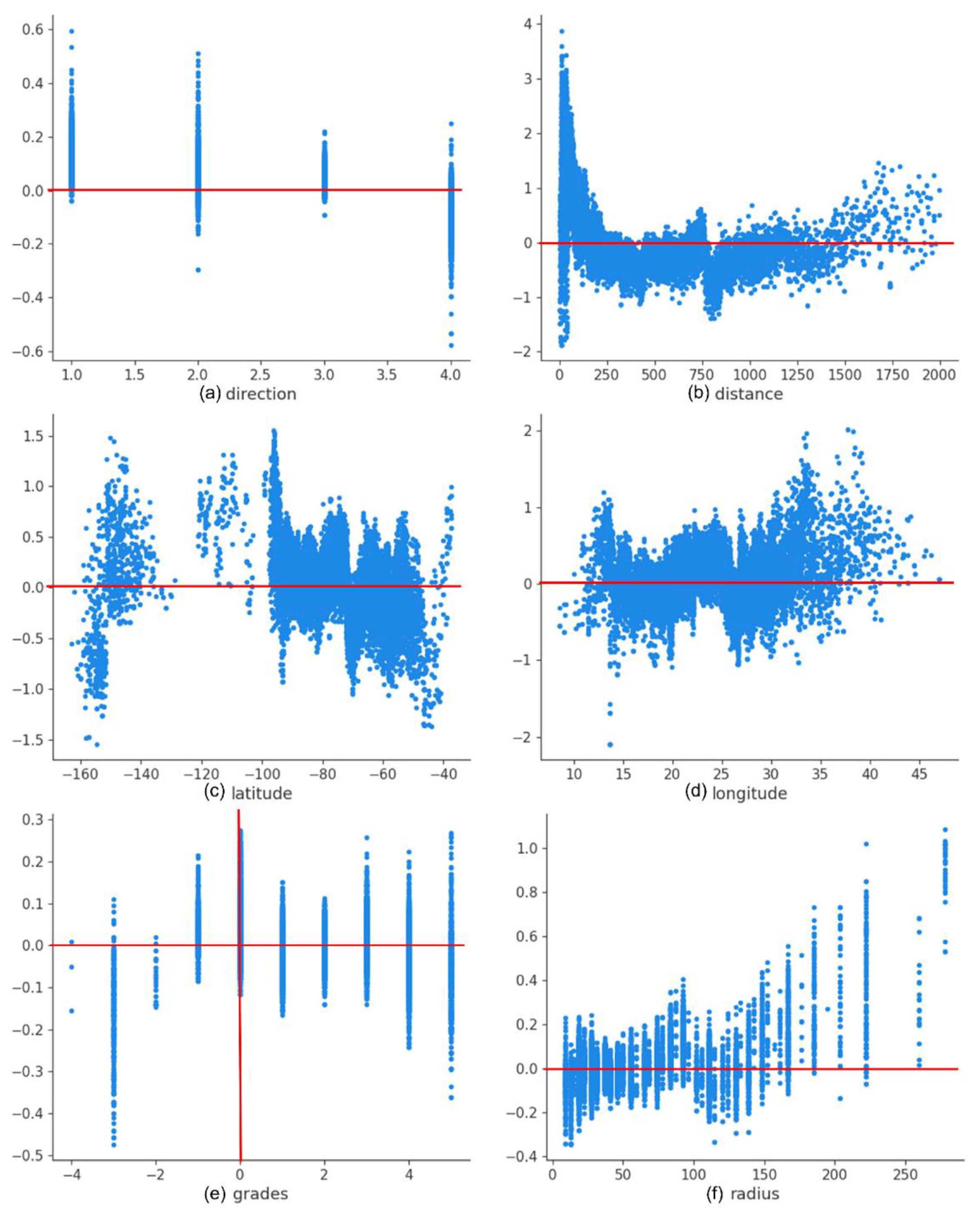
Next, we in detail analyze the relationship between the SHAP values and different factors. Firstly, we investigate the TC parameters (Figure 4). It is vividly shown that it is more likely to form TC ducts on the right-back of the TC tracks compared to the other quadrants (Figure 4a). This conclusion consists with the result obtained by Ding et al.’s [5] work that most ducts are formed on the right side of the TC tracks in the transition zone. However, our results contradict the results from Fei et al. ’s [7] work that ducts are likely to form in every direction around the typhoon center. This may be because of the occasionality caused by the limit of their sample size. From Figure 4b, the probability of ducts first decreases and then increases with the increase in distance between dropsondes and the TC eyes. It is beneficial to the ducts formation in the TC eye; this is mainly because of the subsidence of dryer air masses in the upper layer, and meeting with the humid air in the lower layer. This leads to a high vertical humidity gradient and then forms TC ducts. It is unfavorable for the ducts existence when the dropsonde is out of the eye. With the distance increasing to about 250 km, the ducts probability increases. In Ding et al.’s [5] work, they found that most ducts formed in the transition zone, which also supports our above discussion. Then, when the distance continues to increase, the probability remains unchanged. The geographical location of dropsondes has no obvious effects on the ducts existence (Figure 4c,d). With regard to the TC grade, there is no evident relationship between SHAP value and it. Finally, the probability of TC ducts decreases with the increase in the RMW of the TC.
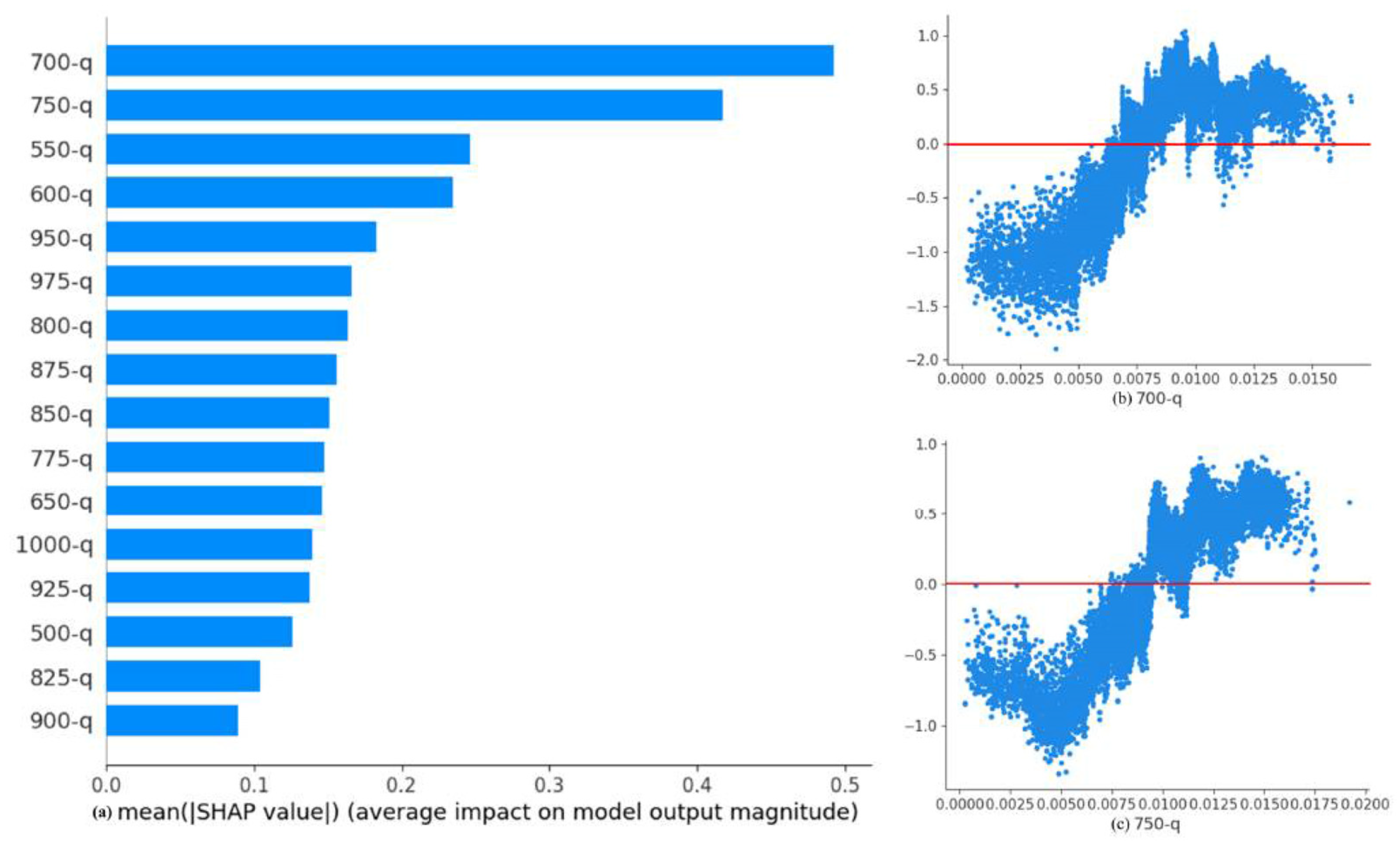
When it comes to the local meteorological parameters, we first compute the average SHAP values of the specific humidity at each pressure level (Figure 5a) and select the most important two levels: 700 hPa and 750 hPa to analyze the SHAP values dependence on them (Figure 5b,c). It was discovered that the probability of ducts decreases with the increase in the humidity at the two levels. It can be inferred that the increase in the humidity makes the humidity gradient between the upper and the lower layer smaller, leading to a decreasing probability.
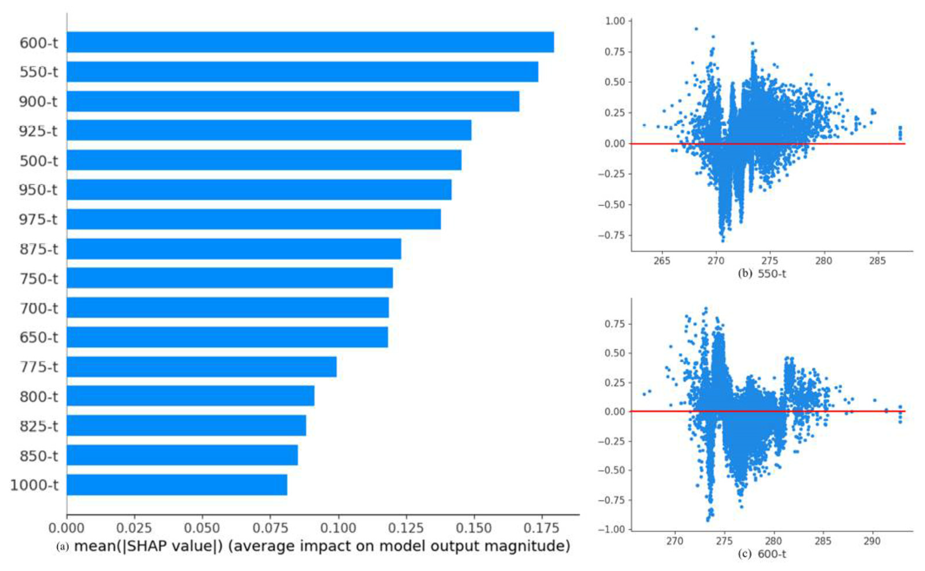
Afterwards, the effects of the temperature at each pressure level are focused (Figure 6a), and the top two important ones: 550 hPa and 600 hPa are selected to research their relationships with SHAP values (Figure 6b,c). It was found that their relationships are relatively complicated with no linear-like relationships presented. However, it can be referred that the condition of 270–275 K at 550 and 600 hPa pressure levels is the most conducive to the ducts’ existence.
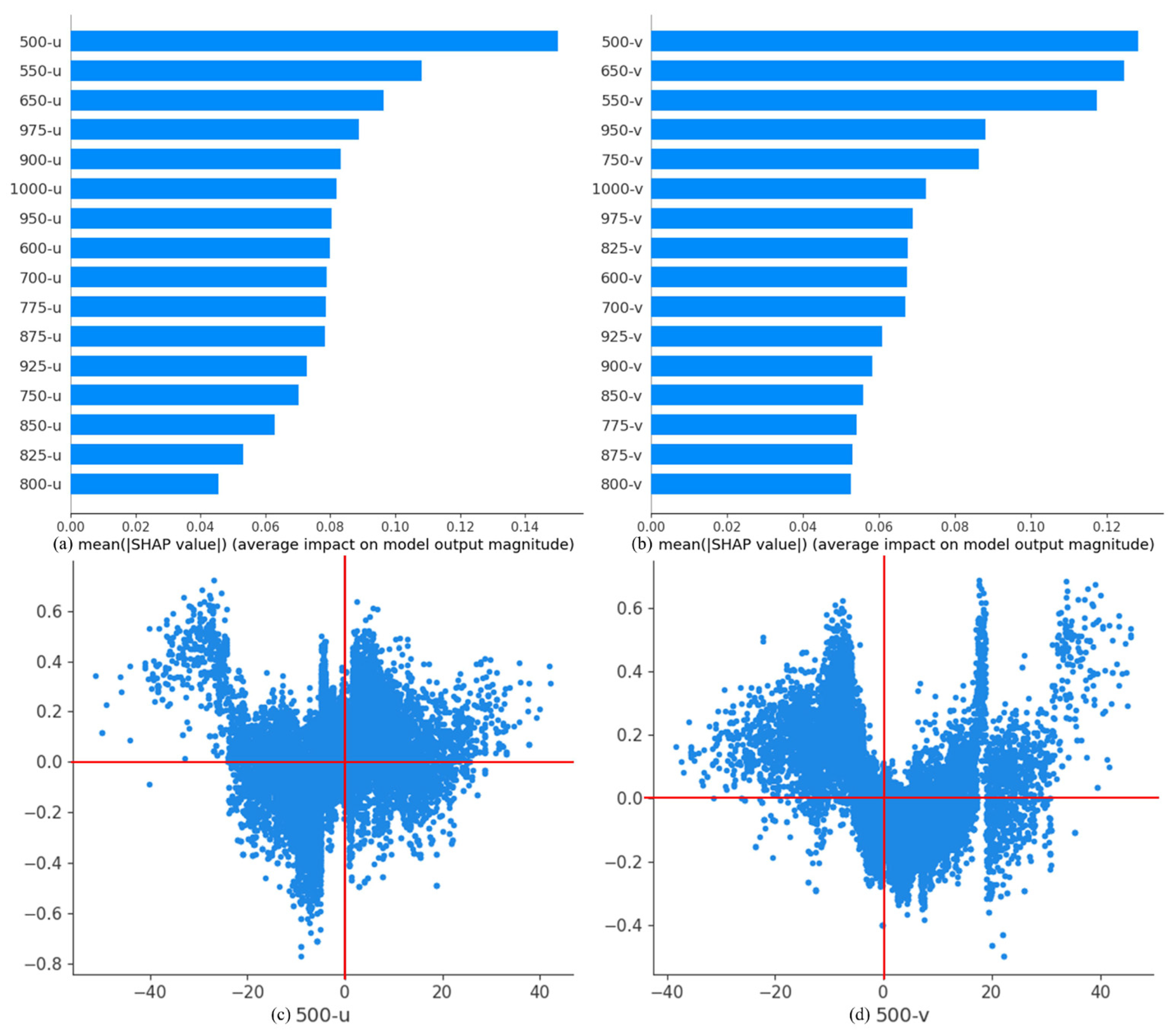
Finally, the effects of zonal and meridional winds at each pressure level are paid attention to (Figure 7a,b). According to Figure 3, the impacts of the winds are totally little, so we combine them into a figure. It is clearly presented that the zonal and meridional winds at 500 hPa pressure level take the first place. Then, the SHAP values’ dependence on them is plotted (Figure 7c,d). No obvious relationship is presented. Generally speaking, the meteorological parameters in the middle and upper layers play a decisive role in the TC ducts formation.

4. Case Analysis in the Tropical Storm Nestor

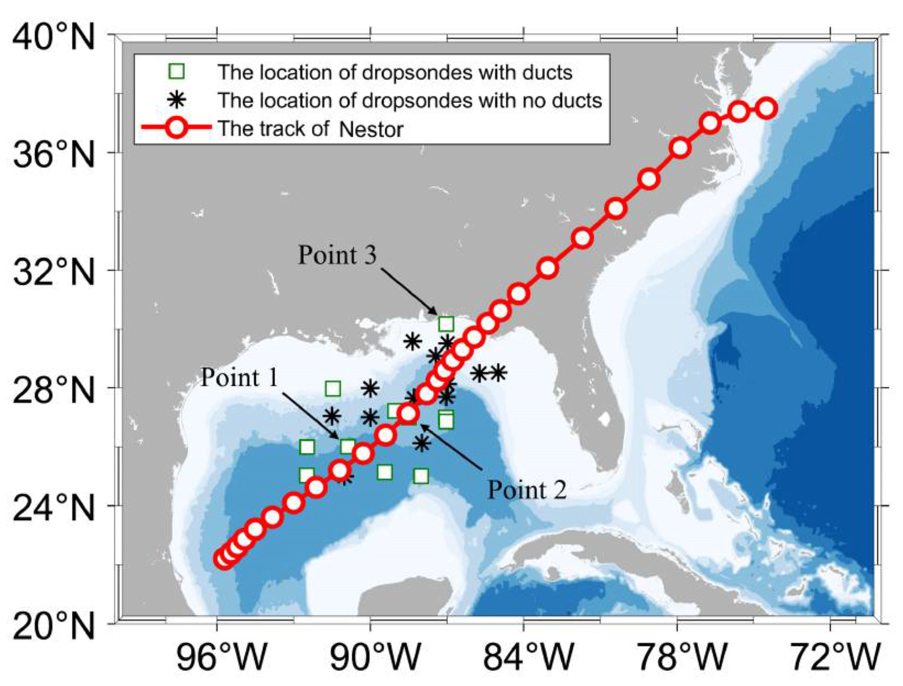
To investigate the relationship between the existence of ducts and the features more specifically, the dropsondes related to the tropical storm Nestor are taken into consideration. Nestor developed into a tropical storm at 1800 UTC 18 October 2019, with its minimum central pressure of 1000 hPa and the RMW of about 92.6 km based on IBTrACS dataset. It was generated in Gulf of Mexico and moved northeastward to the east coast of America. In Nestor, there are totally 25 dropsondes along the track of it, 12 of which detected ducts and 13 detected no ducts. The track of the tropical storm and the locations of the dropsondes with ducts and with no ducts are plotted in Figure 8. In addition, three dropsondes with ducts named, respectively, Point 1, Point 2 and Point 3 for further analysis of the reason for existing ducts are also marked out in this figure. Besides, since the temperature, humidity, etc. are given at pressure levels, a table of pressure-altitude correspondence at normal atmospheric pressure (Table 3) is given to better discuss the change of these variables at different altitudes.
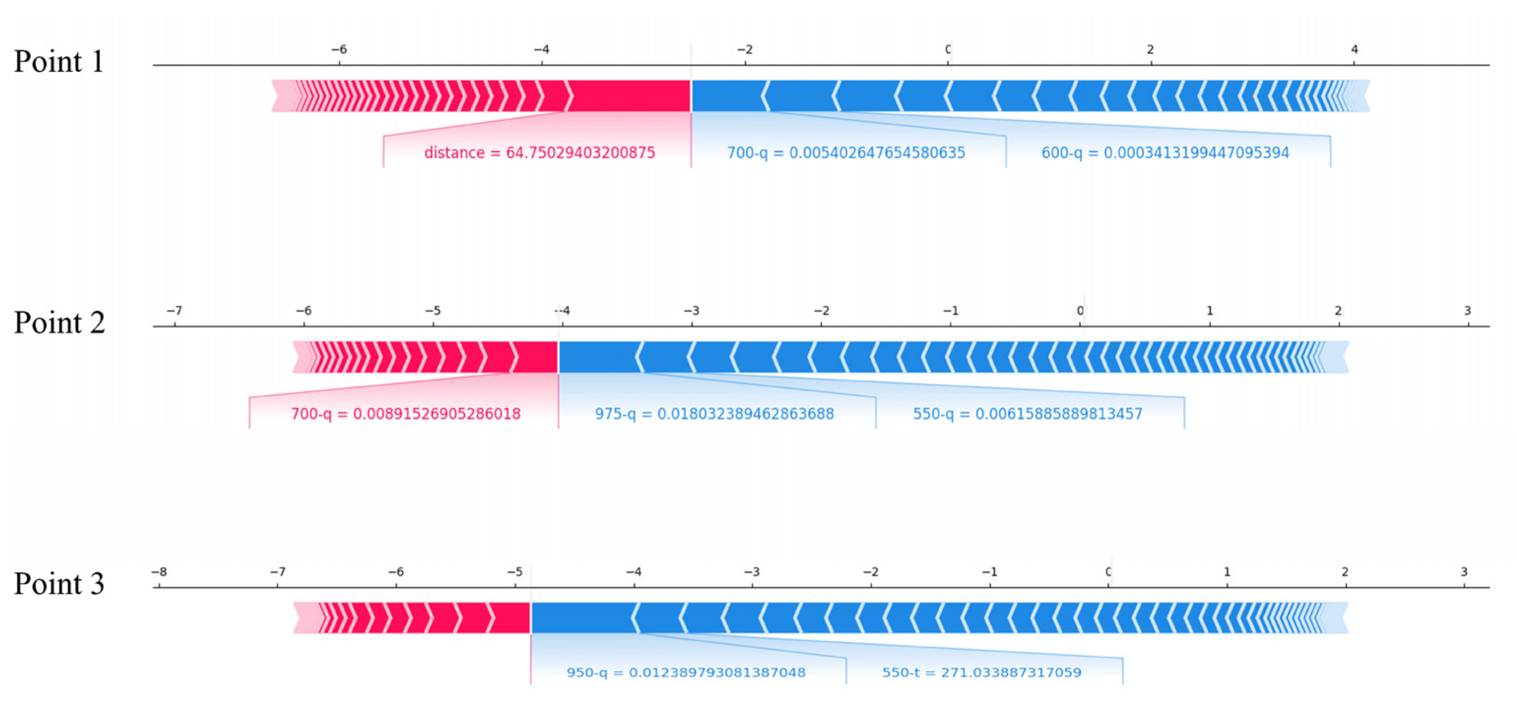
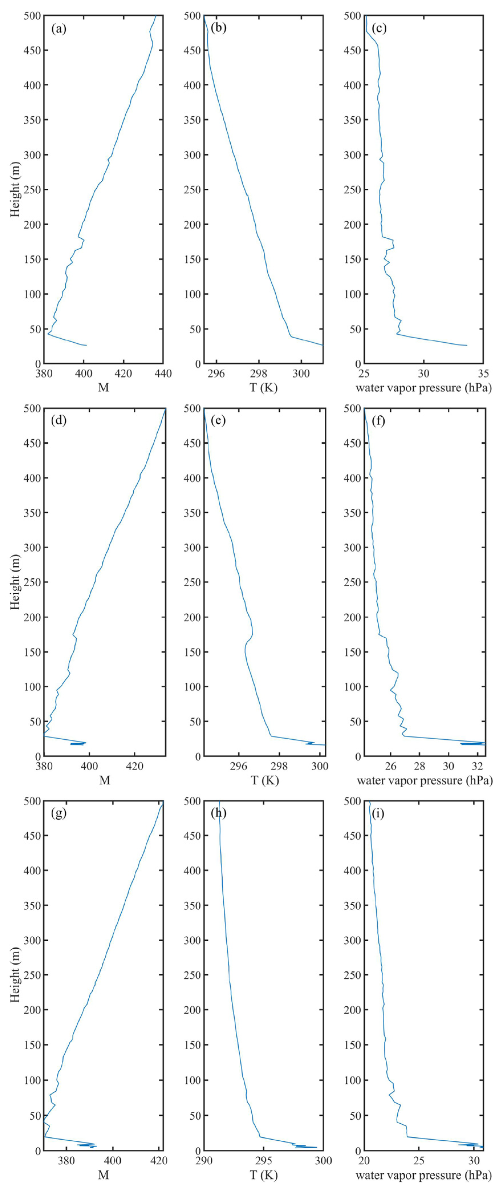
Figure 9 shows the decomposed SHAP values for the individual prediction of the three examples with ducts. Additionally, to explain the reasons for forming duct better, the vertical profile of the modified refractivity, temperature and water vapor pressure at the three points are plotted in Figure 10. In Figure 9, the features that higher the prediction are shown in red and those features that lower the prediction are shown in blue [40]. In the prediction of the existence of ADs, the former represents the decreasing probability of ducts and the latter represents the increasing probability of ducts. Next, a detailed analysis of the reason why ducts exist in these three points is given. For Point 1, the duct here is the surface duct and the duct is formed by the vertical moisture gradient in the lower layer (Figure 10a–c). The features that are most beneficial to the duct formation are the specific humidity at 700 and 600 hPa and the most suppressive feature is the TC-dropsonde distance. As for the TC-dropsonde distance, it is revealed in Section 3 that in the TC, with the distance increasing, the probability of forming ducts decreases rapidly. The existing duct here consists with the conclusion well since the TC-dropsonde distance is smaller than the RMW, which means the dropsonde was in the tropical storm.
For Point 2, the most important features are all specific humidity at different heights, among which the specific humidity at 700 hPa restrains the existence of ducts and the specific humidity at 550 and 975 hPa pressure level are helpful to the duct existence, this may be because this is a surface duct and it is mainly formed by the vertical humidity gradient from Figure 10d–f. Sequentially, the relatively big value of the specific humidity at 950 hPa makes the gradient bigger, while the relatively big value of that at 700 hPa makes the gradient smaller. As has been clarified above, the low humidity in the middle layer can indeed make it easier to form ADs for the big vertical humidity gradient in the atmosphere. For Point 3, the helpful features of the duct existence are specific humidity at 900 hPa and the temperature at 500 hPa. From Figure 10g–i, Tthehe duct is a surface duct, too. Meanwhile, it is caused by the humidity gradient and the high value of specific humidity at 950 hPa pressure level makes the absolute difference between the lower layer and the middle layer bigger. As for the temperature at 550 hPa, this consists with the conclusion obtained in Section 3 that the ducts are more likely to form under the condition of 270–275 K.

5. Conclusions

Based on dropsonde data, in addition to IBTrACS dataset, SRTM15 dataset and ERA-5 reanalysis data, a machine learning method named XGBoost is utilized to predict the TC ducts. Additionally, SHAP is used to interpret the predictions of the model. Through the model’s performance on the testing set, it can be considered that this model has a high reference value for the prediction of TC ducts and ducts in the normal atmosphere. The importance of the factors is sorted according to their SHAP values, and the SHAP values’ dependence on various factors is analyzed. The following conclusions are obtained:
(1) The most important factor in TC ducts formation is the distance between dropsondes and the TC eye. The local meteorological parameters take the second place, in which the humidity and temperature in the upper layer are the most crucial.
(2) The TC ducts are easy to form in the TC eye and the opposite out of the eye. The probability of ducts increases and keeps unchanged with the distance increasing. Secondly, the probability is positively correlated with the RMW. Moreover, the TC ducts are more likely to form in the right-back of the TC tracks.
(3) The increase in the humidity in the middle layer is harmful to the ducts existence. Besides, the situation that the temperature is between 270–275 K in the middle layer is the most favorable for the AD existence.

Author Contributions

Conceptualization, L.H. and X.Z.; methodology, L.H.; software, L.H.; validation, L.H., X.Z. and Y.L.; formal analysis, Y.L.; investigation, L.H.; writing—original draft preparation, L.H.; writing—review and editing, X.Z., Y.L. and P.Y.; supervision, Y.L. and P.Y.; project administration, Y.L. and P.Y.; funding acquisition, X.Z. All authors have read and agreed to the published version of the manuscript.

Funding

This work is supported by the National Natural Science Foundation of China (Grant No. 41875060, 41775027).

Data Availability Statement

The TC-related information in this paper is available on ncdc.noaa.gov/ibtracs/index.php (accessed on 13 June 2022). The dropsonde information can be accessed on https://www.aoml.noaa.gov/hrd/data_sub/dropsonde.html (accessed on 13 June 2022) and the processing software can be downloaded on http://www.eol.ucar.edu/software/aspen (accessed on 13 June 2022). The ERA-5 reanalysis data can be downloaded from https://cds.climate.copernicus.eu/cdsapp#!/home (accessed on 13 June 2022) and the STRM15 elevation data can be accessed on http://www.tuxingis.com (accessed on 13 June 2022).

Conflicts of Interest

The authors declare no conflict of interest. The funders had no role in the design of the study; in the collection, analyses, or interpretation of data; in the writing of the manuscript, or in the decision to publish the results.

References

  1. Von Engeln, A. A Ducting Climatology Derived from the European Centre for Medium-Range Weather Forecasts Global Analysis Fields. J. Geophys. Res. 2004, 109, D18104. [Google Scholar] [CrossRef]
  2. Sun, Z.; Ning, H.; Song, S.; Yan, D. First Observations of Elevated Ducts Associated with Intermittent Turbulence in the Stable Boundary Layer over Bosten Lake, China: Elevated Duct Associated with Turbulence. J. Geophys. Res. Atmos. 2016, 121, 11,201–11,214. [Google Scholar] [CrossRef]
  3. Turton, J.D.; Bennetts, D.A.; Farmer, S.G. An introduction to radio ducting. Meteorol. Mag. 1988, 117, 245–254. [Google Scholar]
  4. Pan, Z.; Liu, S.; Guo, L. The predictions of ducts in south-east coast of China. Chin. J. Radio. Sci. 1996, 11, 58–64. [Google Scholar]
  5. Ding, J.; Fei, J.; Huang, X.; Cheng, X.; Hu, X. Observational Occurrence of Tropical Cyclone Ducts from GPS Dropsonde Data. J. Appl. Meteorol. Climatol. 2013, 52, 1221–1236. [Google Scholar] [CrossRef]
  6. Shi, Y.; Zhang, Q.; Wang, S.; Yang, K.; Yang, Y.; Ma, Y. Impact of Typhoon on Evaporation Duct in the Northwest Pacific Ocean. IEEE Access 2019, 7, 109111–109119. [Google Scholar] [CrossRef]
  7. Fei, J.; Ding, J.; Huang, X.; Cheng, X.; Hu, X. Numerical Study on the Impacts of the Bogus Data Assimilation and Sea Spray Parameterization on Typhoon Ducts. Acta Meteorol Sin. 2013, 27, 308–321. [Google Scholar] [CrossRef]
  8. von Engeln, A.; Nedoluha, G.; Teixeira, J. An Analysis of the Frequency and Distribution of Ducting Events in Simulated Radio Occultation Measurements Based on Ecmwf Fields: Distribution of Ducting Events. J. Geophys. Res. 2003, 108, D21. [Google Scholar] [CrossRef]
  9. Yang, K.; Zhang, Q.; Shi, Y. Interannual Variability of the Evaporation Duct over the South China Sea and Its Relations with Regional Evaporation: Relate Evaporation Duct to Evaporation. J. Geophys. Res. Oceans 2017, 122, 6698–6713. [Google Scholar] [CrossRef]
  10. Manjula, G.; Roja Raman, M.; Venkat Ratnam, M.; Chandrasekhar, A.V.; Vijaya Bhaskara Rao, S. Diurnal Variation of Ducts Observed over a Tropical Station, Gadanki, Using High-Resolution GPS Radiosonde Observations: Diurnal Variation of Ducts. Radio Sci. 2016, 51, 247–258. [Google Scholar] [CrossRef]
  11. Zhao, X.; Wang, D.; Huang, S.; Huang, K.; Chen, J. Statistical Estimations of Atmospheric Duct over the South China Sea and the Tropical Eastern Indian Ocean. Chin. Sci. Bull. 2013, 58, 2794–2797. [Google Scholar] [CrossRef]
  12. Dockery, G.D. Modeling Electromagnetic Wave Propagation in the Troposphere Using the Parabolic Equation. IEEE Trans. Antennas Propagat. 1988, 36, 1464–1470. [Google Scholar] [CrossRef]
  13. Cook, J. A Sensitivity Study of Weather Data Inaccuracies on Evaporation Duct Height Algorithms. Radio Sci. 1991, 26, 731–746. [Google Scholar] [CrossRef]
  14. Li, P.; Zhou, K.; Lu, X.; Yang, S. A Hybrid Deep Learning Model for Short-Term PV Power Forecasting. Appl. Energy 2020, 259, 114216. [Google Scholar] [CrossRef]
  15. Shen, Z.; Zhang, Y.; Lu, J.; Xu, J.; Xiao, G. A Novel Time Series Forecasting Model with Deep Learning. Neurocomputing 2020, 396, 302–313. [Google Scholar] [CrossRef]
  16. Ham, Y.-G.; Kim, J.-H.; Luo, J.-J. Deep Learning for Multi-Year ENSO Forecasts. Nature 2019, 573, 568–572. [Google Scholar] [CrossRef]
  17. Shen, M.; Keenlyside, N.; Selten, F.; Wiegerinck, W.; Duane, G.S. Dynamically Combining Climate Models to “Supermodel” the Tropical Pacific. Geophys. Res. Lett. 2016, 43, 359–366. [Google Scholar] [CrossRef]
  18. Guo, P.; Kuo, Y.-H.; Sokolovskiy, S.V.; Lenschow, D.H. Estimating Atmospheric Boundary Layer Depth Using COSMIC Radio Occultation Data. J. Atmos. Sci. 2011, 68, 1703–1713. [Google Scholar] [CrossRef]
  19. Hwang, J.; Orenstein, P.; Cohen, J.; Pfeiffer, K.; Mackey, L. Improving subseasonal forecasting in the western US with machine learning. In Proceedings of the 25th ACM SIGKDD International Conference on Knowledge Discovery & Data Mining, Anchorage, AK, USA, 25 July 2019; pp. 2325–2335. [Google Scholar]
  20. Gao, S.; Huang, Y.; Zhang, S.; Han, J.; Wang, G.; Zhang, M.; Lin, Q. Short-Term Runoff Prediction with GRU and LSTM Networks without Requiring Time Step Optimization during Sample Generation. J. Hydrol. 2020, 589, 125188. [Google Scholar] [CrossRef]
  21. Zhu, X.; Li, J.; Zhu, M.; Jiang, Z.; Li, Y. An Evaporation Duct Height Prediction Method Based on Deep Learning. IEEE Geosci. Remote Sens. Lett. 2018, 15, 1307–1311. [Google Scholar] [CrossRef]
  22. Han, J.; Wu, J.-J.; Zhu, Q.-L.; Wang, H.-G.; Zhou, Y.-F.; Jiang, M.-B.; Zhang, S.-B.; Wang, B. Evaporation Duct Height Nowcasting in China’s Yellow Sea Based on Deep Learning. Remote Sens. 2021, 13, 1577. [Google Scholar] [CrossRef]
  23. Chen, T.; Guestrin, C. XGBoost: A Scalable Tree Boosting System. In Proceedings of the 22nd ACM SIGKDD International Conference on Knowledge Discovery and Data Mining, San Francisco, CA, USA, 13 August 2016; pp. 785–794. [Google Scholar]
  24. Dong, H.; Xu, X.; Wang, L.; Pu, F. Gaofen-3 PolSAR Image Classification via XGBoost and Polarimetric Spatial Information. Sensors 2018, 18, 611. [Google Scholar] [CrossRef] [PubMed]
  25. Zhao, W.P.; Li, J.; Zhao, J.; Zhao, D.; Lu, J.; Wang, X. XGB Model: Research on Evaporation Duct Height Prediction Based on XGBoost Algorithm. Radio Eng. 2020, 29, 81–93. [Google Scholar] [CrossRef]
  26. Lundberg, S.M.; Lee, S.-I. A Unified Approach to Interpreting Model Predictions. In Proceedings of the 31st International Conference on Neural Information Processing Systems, Long Beach, CA, USA, 4–9 December 2017; pp. 4768–4777. [Google Scholar]
  27. Smith, E.K.; Weintraub, S. The Constants in the Equation for Atmospheric Refractive Index at Radio Frequencies. Proc. IRE 1953, 41, 1035–1037. [Google Scholar] [CrossRef]
  28. NOAA-DHA: Long-Term NOAA Dropsonde Hurricane Archive. Version 2.0; UCAR/NCAR–Earth Observing Laboratory: Boulder, CO, USA, 2017. [CrossRef]
  29. Zhu, M.; Atkinson, B.W. Simulated Climatology of Atmospheric Ducts Over the Persian Gulf. Bound.-Layer Meteorol. 2005, 115, 433–452. [Google Scholar] [CrossRef]
  30. Knapp, K.R.; Kruk, M.C.; Levinson, D.H.; Diamond, H.J.; Neumann, C.J. The International Best Track Archive for Climate Stewardship (IBTrACS): Unifying tropical cyclone best track data. Bull. Am. Meteorol. Soc. 2010, 91, 363–376. [Google Scholar] [CrossRef]
  31. Kursinski, E.R.; Hajj, G.A.; Leroy, S.S.; Herman, B. The GPS radio occultation technique. Terr. Atmos. Oceanic Sci. 2000, 11, 53–114. [Google Scholar] [CrossRef]
  32. Peng, L.R.; Shu, S. Analysis on structure of Typhoon Longwang based on GPS dropsonde data. Chin. J. Trop. Meteor. 2010, 26, 13–21. [Google Scholar]
  33. Abdullah, A.Y.M.; Masrur, A.; Adnan, M.S.G.; Baky, M.A.A.; Hassan, Q.K.; Dewan, A. Spatio-Temporal Patterns of Land Use/Land Cover Change in the Heterogeneous Coastal Region of Bangladesh between 1990 and 2017. Remote Sens. 2019, 11, 790. [Google Scholar] [CrossRef]
  34. Mai, Y.; Sheng, Z.; Shi, H.; Liao, Q. Using Improved XGBoost Algorithm to Obtain Modified Atmospheric Refractive Index. Int. J. Antennas Propag. 2021, 2021, 5506599. [Google Scholar] [CrossRef]
  35. Pedregosa, F.; Varoquaux, G.; Gramfort, A.; Michel, V.; Thirion, B.; Grisel, O.; Blondel, M.; Prettenhofer, P.; Weiss, R.; Dubourg, V.; et al. Scikit-Learn: Machine Learning in Python. J. Mach. Learn. Res. 2011, 12, 2825–2830. [Google Scholar]
  36. Cohen, J. A Coefficient of Agreement for Nominal Scales. Educ. Psychol. Meas. 1960, 20, 37–46. [Google Scholar] [CrossRef]
  37. Landis, J.R.; Koch, G.G. The Measurement of Observer Agreement for Categorical Data. Biometrics 1977, 33, 159–174. [Google Scholar] [CrossRef]
  38. Lundberg, S. Interpretable Machine Learning with XGBoost. Available online: https://towardsdatascience.com/interpretable-machine-learning-with-xgboost-9ec80d148d27 (accessed on 1 August 2022).
  39. Shapley, L.S. Quota solutions op n-person games1. Contrib. Theory Games (AM-28) Vol. II 2016, 28, 343. [Google Scholar]
  40. Dataman: Explain Your Model with the SHAP Values–Towards Data Science. Available online: https://towardsdatascience.com/explain-your-model-with-the-shap-values-bc36aac4de3d (accessed on 1 August 2022).
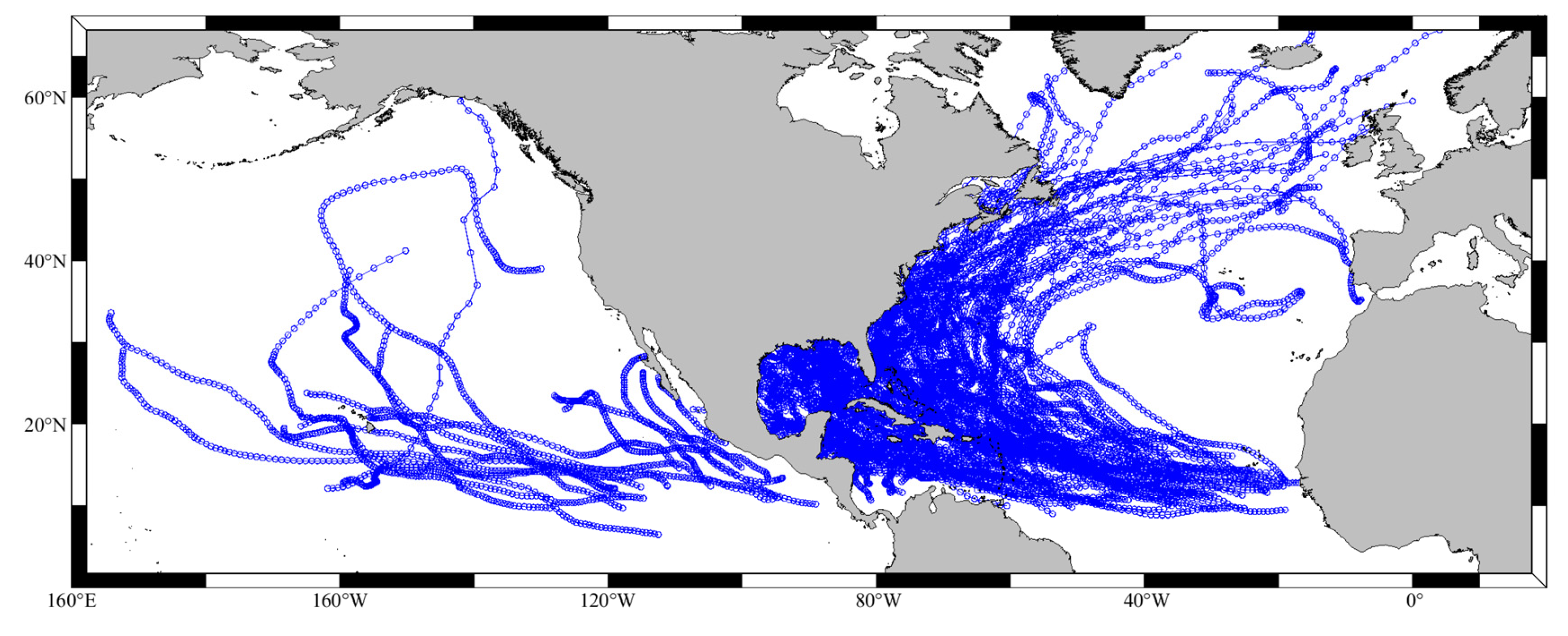
Figure 1. The tracks of 164 hurricanes in the eastern Pacific and North Atlantic during 1996–2020.
Remotesensing 14 03952 g001
Figure 2. XGBoost model and SHAP interpretation construction diagram.
Remotesensing 14 03952 g002
Figure 3. The top 20 most important features are obtained by sorting all of them according to SHAP values based on the total dataset.
Remotesensing 14 03952 g003
Figure 4. The SHAP dependence plot for TC parameters and the location of dropsondes.
Remotesensing 14 03952 g004
Figure 5. The SHAP values ranking of the humidity at pressure levels and dependence for the two most important ones.
Remotesensing 14 03952 g005
Figure 6. The SHAP values ranking of the temperature at pressure levels and dependence for the two most important ones.
Remotesensing 14 03952 g006
Figure 7. The SHAP values ranking of the winds at pressure levels and dependence for the two most important ones.
Remotesensing 14 03952 g007
Figure 8. The track of the tropical storm Nestor and the location of dropsondes with ducts and with no ducts. Point 1, 2 and 3 represent the three dropsondes for further analysis of the reason for existing ducts.
Remotesensing 14 03952 g008
Figure 9. Decomposed SHAP values for the individual prediction of three examples with ducts.
Remotesensing 14 03952 g009
Figure 10. The vertical profile of modified refractivity, temperature and water vapor pressure at Point 1, 2 and 3. (ac) represent Point 1. (df) represent Point 2. (gi) represent Point 3.
Remotesensing 14 03952 g010
Table 1. The features used for the duct existence prediction.
CategoryFeature Name
Meteorological parametersSpecific humidity (1000–500 hPa)
Temperature (1000–500 hPa)
Zonal winds (1000–500 hPa)
Meridional winds (1000–500 hPa)
TC parametersTC grades
TC RMW
Dropsonde quadrant
TC-dropsonde distance
Location parametersLatitude
Longitude
Table 2. The parameter combination with the best test performance for XGBoost.
ParameterValue
Learning_rate0.05
Max_depth9
N_estimators3000
Min_child_weight1
Reg_lamda1
Reg_alpha0.1
Subsample0.9
Colsample_bytree0.9
Gamma0
Table 3. The pressure-altitude correspondence at normal atmospheric pressure.
Pressure Levels (hPa)Altitudes (km)
5004.94
5504.42
6003.48
6503.06
7002.67
7502.31
7751.98
8001.68
8251.41
8501.17
8750.95
9000.76
9250.60
9500.46
9750.24
10000.10
Publisher’s Note: MDPI stays neutral with regard to jurisdictional claims in published maps and institutional affiliations.