
A Retrospective Satellite Analysis of the June 2012 North American Derecho


1
NOAA/NESDIS Center for Satellite Applications and Research (STAR), College Park, MD 20740, USA
2
Physics Department, University of Maryland, Baltimore County, Baltimore, MD 21250, USA
*
Author to whom correspondence should be addressed.
Remote Sens. 2022, 14(14), 3479; https://doi.org/10.3390/rs14143479
Submission received: 1 June 2022
/
Revised: 13 July 2022
/
Accepted: 15 July 2022
/
Published: 20 July 2022
(This article belongs to the Special Issue Satellite Data Application, Validation, and Calibration for Atmospheric Observation II)
Abstract
:The North American Derecho of 29–30 June 2012 exhibits many classic progressive and serial derecho features. It remains one of the highest-impact derecho-producing convective systems (DCS) over CONUS since 2000. This research effort enhances the understanding of the science of operational forecasting of severe windstorms through examples of employing new satellite and ground-based microwave and vertical wind profile data. During the track of the derecho from the upper Midwestern U.S. through the Mid-Atlantic region on 29 June 2012, clear signatures associated with a severe MCS were apparent in polar-orbiting satellite imagery, especially from the EPS METOP-A Microwave Humidity Sounder (MHS), Defense Meteorological Satellite Program (DMSP) Special Sensor Microwave Imager Sounder (SSMIS), and NASA TERRA Moderate Resolution Imaging Spectroradiometer (MODIS). In addition, morning (descending node) and the evening (ascending node) METOP-A Infrared Atmospheric Sounding Interferometer (IASI) soundings are compared to soundings from surface-based Radiometrics Corporation MP-3000 series microwave radiometer profilers (MWRPs) along the track of the derecho system. The co-located IASI and MWRP soundings revealed a pre-convective environment that indicated a favorable volatile tropospheric profile for severe downburst wind generation. An important outcome of this study will be to formulate a functional relationship between satellite-derived parameters and signatures, and severe convective wind occurrence. Furthermore, a comprehensive approach to observational data analysis involves both surface- and satellite-based instrumentation. Because this approach utilizes operational products available to weather service forecasters, it can feasibly be used for monitoring and forecasting local-scale downburst occurrence within derecho systems, as well as larger-scale convective wind intensity associated with the entire DCS.
1. Introduction
1.1. Background
Downbursts are strong downdrafts that induce an outburst of damaging winds at or near the ground, and a microburst is a very small downburst with an outflow diameter of less than 4 km and a lifetime of less than 5 min [1,2]. The dangers posed by convective storm-generated downbursts have been extensively documented. Severe windstorms (i.e., widespread convective wind gusts >25.7 m s−1 (50 kt)) resulting from mesoscale convective systems (MCSs) cause significant disruption to society, including widespread power outages, tree and structural damage, and transportation accidents that affect multi-state regions and metropolitan areas along their track. Among them, a derecho, defined by Johns and Hirt [3] as a long-lived, widespread severe convective windstorm, is composed of numerous downbursts organized into clusters or families of clusters. Derechos can produce winds above hurricane force along a track that may exceed several hundred (400) kilometers [3]. Derived from a dataset presented by Ashley and Mote [4], we found that, between 1987 and 2002, severe convective windstorms resulted in a total property loss of over $3 billion in the United States, with an average loss per event of $96 million. Moreover, between 1986 and 2003, severe convective windstorms were responsible for a total of 153 deaths and 2605 injuries, proving to be deadlier and more hazardous than the low-end (F-0/F-1 intensity) tornado outbreaks that occurred during the same period and resulted in only 71 deaths [4]. Because these events are severe, it is critical to understand the factors that lead to the downbursts and utilize all available observations to monitor and forecast their development.
Proctor [5] and Pryor [6] noted that convective windstorm potential has been traditionally expressed as a grouping of stability parameters relevant for downburst generation. These include lower-to-mid-tropospheric temperature and equivalent potential temperature (theta-e) lapse rates, vertical relative humidity differences, and the amount of convective available potential energy (CAPE) in the troposphere. Some factors that increase the likelihood of severe convective winds are (1) an elevated mixed layer that promotes instability by generating powerful storm updrafts and downdrafts [7] and (2) a rear-inflow jet (RIJ) into an MCS [8,9] which channels unsaturated mid-tropospheric air into the leading convective storm line. The establishment of an elevated, ascending front-to-rear flow originating from deep, moist convection, overlying a strong and deep outflow-induced cold pool has been found to generate and sustain a robust rear inflow jet [9]. Other factors documented by Proctor [5] and Srivastava [10] can reduce the likelihood of severe convective winds, such as the presence of a lower-tropospheric temperature inversion and a surface-based layer of unsaturated air that reduces virtual temperature.
During the morning of 29 June 2012, an area of multicell convective storms developed over Iowa north of a stationary frontal boundary and in an environment favorable for elevated convection [11]. The area of storms subsequently organized into a quasi-linear convective system (QLCS) as it tracked into northern Illinois and convective downdrafts were able to penetrate a shallow surface-based stable layer. The system then evolved into a bow echo [12] during the afternoon and tracked rapidly southeastward over the Ohio Valley to the Mid-Atlantic coast by late evening. This extraordinary derecho-producing convective system (DCS) event resulted in 22 deaths and nearly a thousand severe wind reports from northern Illinois to the Atlantic Coast [13]. This system was more typical of a warm-season progressive derecho, associated with a major heatwave and an elevated mixed layer [7]. During the evening of 29 June, the derecho tracked rapidly eastward across the mountains of West Virginia (WV), western Virginia (VA), southwest Pennsylvania (PA), and western Maryland (MD). The derecho’s effects were particularly formidable in the Washington, DC–Baltimore, MD corridor, where measured wind gusts of 31–36 m s−1 (60–70 kt) severed numerous overhead electrical feeders. Overall, this derecho resulted in power loss to over four million customers and caused $3.7 billion in property loss, greater than the total loss for all convective windstorms that occurred between 1987 and 2002 [14].
The original NOAA service assessment report of the June 2012 North American Derecho [14] did not incorporate any analysis of operational meteorological satellite imagery or sounder-derived data, or analysis of ground-based profiler sounding datasets that would have provided beneficial guidance on atmospheric stability and storm structural evolution. Therefore, on the ten-year anniversary of this historic and record-breaking weather event, we present a discussion of the science of operational forecasting of severe windstorms through examples of employing new satellite and ground-based microwave and vertical wind profile data. Accordingly, this paper is organized as follows: Section 1 provides a brief background of severe convective windstorm theory and discusses windstorm genesis and evolution. Section 2 summarizes the instrumentation and measurement application methodology for this event study. As an example of the coordinated use of surface- and satellite-based observational instrumentation, Section 3 presents a discussion of the genesis, evolution, and intensification of the DCS from the Midwestern U.S. to the Mid-Atlantic coastal region, emphasizing its impact on the Baltimore, Maryland–Washington, DC corridor. Finally, Section 4 provides a discussion of the operational forecasting implications of this DCS study.
1.2. Storm Microphysical and Thermodynamic Processes
Moller [15] states the standard NOAA/National Weather Service (NWS) definition of a severe thunderstorm that includes damaging winds with gusts of 26 m s−1 (50 kt) or greater and hail with a diameter of 0.02 m or greater. Severe thunderstorms are most identifiable in weather radar imagery in which a large concentration of ice-phase precipitation within a volume results in high reflectivity resulting from increased backscattering. Downdraft severity is governed by phase change and the loading of ice-phase precipitation. A prototypical conceptual model of a deep moist convective (DMC) storm is shown in Figure 1. Srivastava [16] found that precipitation in the form of ice increases the convective downdraft intensity. This effect increases with precipitation content and the stability of the environmental lapse rate of temperature. The power of the downdraft also increases in proportion to the relative concentration of smaller particles. Condensate loading [16], sometimes combined with subsaturated air entrainment in the storm’s middle level [17], initiates the convective downdraft. In conjunction with precipitation loading, the melting of frozen hydrometeors and subcloud evaporation of liquid precipitation results in the cooling and negative buoyancy that accelerate the downdraft in the unsaturated layer promoted by a significant temperature lapse rate [16].
Knupp [17,18] refined the understanding of downburst generation physical and dynamic processes. The author noted that low-level downdrafts are closely controlled by the arrival of precipitation at low levels. In the storm’s middle levels, air flows quasi-horizontally around the updraft flanks and converges into the downshear flank, referred to as the wake region, where precipitation at middle levels (where it is grown most effectively) is then allowed to descend to lower levels. The intrusion of drier air into the wake’s precipitation region also enhances the evaporation/sublimation process that is most effective below the melting level. Convergence within the downshear wake is thus instrumental in transporting precipitation into the downshear flank. Therefore, a comprehensive understanding of the downdraft initiation process is closely related to the precipitation initiation and transport process within clouds and is observable in passive microwave (MW) imagery, as shown in this study in later figures. Such processes depend not only on vertical temperature and moisture profiles but also on vertical environmental wind profiles. Knupp [18] subsequently identified the protrusion echo produced by settling hydrometeors from a line of weak updrafts formed in association with a low-level confluence located east of the storm core and was indirectly connected to the strong core downdraft. Initial bowing of the echo [12] was associated with the early microburst activity, a characteristic observed in other case studies. The inference of downburst occurrence can be successfully applied by the synergistic use of satellite-based passive MW and ground-based Doppler radar data and imagery.
1.3. Storm Dynamic Processes
From Weisman et al. [19] as a departure point, Weisman [9] explored the role of vertical wind shear and buoyancy in the generation of a rear inflow jet and visualized the associated conceptual model of this process. Weisman [9] noted that rear inflow is generated in response to the development of an upshear-tilted updraft as the horizontal buoyancy gradients along the back edge of the expanding system create a circulation that draws midlevel air in from the rear. The rear inflow jet system can take two forms, descending or elevated. For a descending-jet system, the convective circulation is characterized by an updraft current that ascends gradually above a spreading surface cold pool, with light-to-moderate convective and stratiform rainfall extending well behind the leading edge of the cold pool. This structure is often associated with a decaying system. The gust-front lifting is not strong or deep enough to regenerate new convective cells, and the mesoscale circulation slowly weakens. However, for an elevated-jet system, the circulation is dominated by strong, erect updrafts along the leading edge of the surface cold pool. The updraft current spreads rapidly rearward above 7000–8000 m above ground level. Moderate-to-heavy convective rainfall exists at the system’s leading edge, with lighter rainfall extending to the rear. This structure tends to be longer-lived than the descending-jet case, as the deeper gust-front lifting regularly regenerates strong convective cells.
The rear-inflow jet represented a new, potentially significant horizontal vorticity source that must be included when diagnosing various circulation sources’ relative importance. Specifically, a rear-inflow jet that descends and spreads along the surface is characterized by the same sign of horizontal vorticity generated by the cold pool, thereby accentuating the cold pool circulation. An elevated rear-inflow jet is characterized by the opposite sign of horizontal vorticity generated by the cold pool (up to jet level), thereby accentuating the ambient vertical shear effects. Since significant rear-inflow characteristically develops after the cold-pool circulation overwhelms the ambient shear, a surface jet’s development reinforces the upshear-tilting process weakens the system. However, an elevated rear-inflow jet’s development reverses this process, promoting powerful, upright convective cells along the cold pool’s leading edge. Johns [20] built on the basis established by previous observational and modeling studies of environmental conditions associated with the development and maintenance of bow echo-induced damaging winds, focused on parameters related to storm outflow and updraft strengths. Specifically, wind speeds and relative humidity values in the mid-levels (related to outflow strength) and instability (related to updraft strength) were examined. The results indicated that these parameters exhibit a wide range of values when considering all bow echo situations in which damaging winds are reported.
Further, combinations of wind speeds in the mid-levels and instability tend to vary with the season and the synoptic situation. For example, as detailed by Johns [20] and Moller [15], when powerful winds are present in the mid-levels, bow echo development has been observed in only marginally unstable environments. Bow echo events associated with the powerful wind-marginal instability combination typically occur with strong, rapidly moving low-pressure systems (“dynamic” synoptic pattern) in the year’s colder months. On the other hand, events associated with the relatively weak wind-extreme instability combination typically occur along a quasi-stationary thermal boundary in relatively stagnant weather regimes (“warm season” synoptic pattern) in late spring or summer. Many bow echo wind events are associated with wind-instability combinations between the extremes. Some of these events are related to synoptic patterns that do not match the prototypical pattern sufficiently.
Another dynamical aspect of severe MCSs, especially relevant to the June 2012 Derecho, is the development and evolution of storm-scale horizontal circulations that may be detectable by satellite- and ground-based remote sensing instrumentation. Fritch and Forbes [21] identify and outline the physical process of these storm-scale circulation patterns. For example, the divergence averaged over the convective region is characterized by convergence (negative divergence) in the lower troposphere and (positive) divergence in the upper troposphere. The profile typically shows convergence in the middle troposphere in the stratiform region, with a maximum at about the 600–700 mb level, with divergence at upper and lower levels. The maximum divergence is at high levels, where both the convective and stratiform regions are divergent. MCSs are sufficiently large and long-lived that the earth’s rotation becomes a factor in determining dynamical structure and circulation, which should tend to follow the balanced dynamical constraints derivable from potential vorticity (PV) concepts. Negative and positive PV anomalies within the MCS structure often produce storm upper-level anticyclonic outflow and the mid-level mesoscale convective vortex (MCV), respectively. The Davis and Weisman [22] (Equation 1.1) formulation of PV applicable to large MCSs can be approximated as PV ≈ Del ∙ (θ) ≈ Del(θ) ≈ ∂θ/∂P, so that PV~∂θ/∂P, assuming conservation of absolute vorticity over the relatively local time and space scales of the existence of the MCV over northern Ohio associated with the June 2012 Derecho event. An alternative explanation of the evolution of MCV development proceeds from the circulation theorem and is derived by Skamarock et al. [23]. This derivation establishes a direct proportionality between vertical buoyancy and circulation in which increasing positive buoyancy (i.e., CAPE) in the MCS environment can increase midlevel cyclonic circulation in the trailing stratiform precipitation region. Both processes will be discussed further in Section 3 to demonstrate meteorological satellite detectability of these features.
2. Materials and Methods
Surface-based measurements in the infrared and microwave regions of the electromagnetic spectrum provide important environmental parameters for monitoring atmospheric stability and mesoscale and microphysical processes associated with convective storm development. Over the continental United States (CONUS), traditional datasets applied to both operational downburst monitoring and prediction, as well as product validation, include surface-based observations of atmospheric parameters (i.e., temperature, humidity, wind speed/direction, sky condition, precipitation accumulation, etc.) from NWS/FAA aviation routine meteorological reports (METAR) stations, mesonetwork (mesonet) stations, radiosonde observations, and meteorological Doppler radar reflectivity and velocity measurements. In effect, surface weather observation and analysis represent an important primary step in the convective storm diagnosis process and in determining of the possibility of organization into larger-scale MCSs and QLCSs.
In addition, as noted in Figure 2, vertical temperature and moisture sounding datasets generated by surface-based MP-3000 series microwave radiometer profilers (MWRPs), manufactured by Radiometrics Corporation, provide routine monitoring of thermodynamic patterns in both the pre-convective and storm environments [24]. As outlined in Figure 2 and shown in Figure 3 and Figure 4, the June 2012 North American Derecho was observed simultaneously by the microwave sensors onboard polar-orbiting meteorological satellites, vertical sounding profiles generated from the Infrared Atmospheric Sounding Interferometer (IASI), NEXRAD systems, and MWRPs. Remarkably, as demonstrated in Figure 4, Hovmӧller diagrams of equivalent potential temperature (θe), with overlying plots of θe lapse rate (LR or Γθe), were derived from four consecutive network MWRPs at Cedar Falls, Iowa, Cleveland, Ohio, and Germantown, and Beltsville, Maryland, respectively. θe is a preferred thermodynamic quantity since its conservation is consistent with upward motions resulting in saturation and cloud layer destabilization. In addition, negative vertical θe lapse rates (i.e., Γθe = ∂θe/∂z < 0) indicate the presence of potential instability (PI) [25]. These diagrams were instrumental in illustrating the evolution of thermodynamic and stability conditions surrounding the DCS, and storm structural characteristics of the DCS as it progressed through its life cycle stages.
MWRPs observe atmospheric brightness temperatures in 21 frequency channels from 22–30 GHz (K-band) and 14 channels from 51 to 59 GHz (V-band) and retrieve temperature and humidity soundings up to 10,000 m height with a vertical resolution of 50 m below 500 m AGL and a resolution of 100 m between 500 and 2000 m and 250 m between 2000 and 10,000 m AGL. The MWRP exploits the 30 to 50 GHz transmission window to retrieve water vapor profiles while using the absorption band near 60 GHz for temperature sensing. The MWRP employs the neural network (NN) inversion retrieval method, as described in Solheim et al. [28] and Cimini et al. [29], trained with a large dataset of profiles generated from historical datasets of operational radiosondes. Vertical temperature and humidity profiles are often applied to calculate CAPE, temperature lapse rates, and other atmospheric stability indices to determine the presence of conditional instability (CI) and potential instability. The parcel choice for CAPE computation was an important consideration for this study. The most unstable parcel CAPE (MUCAPE) was selected due to its universality and versatility as an estimator of positive buoyancy for both elevated and surface-based convection [30] and thus applicable to the range of thermodynamic environments observed during this derecho event. Accordingly, this paper demonstrates thunderstorm downburst potential applications of the CAPE-dependent microburst windspeed potential index (MWPI) [6] as calculated from MWRP and satellite sounding datasets.
Data collection, processing, and visualization follow the methodology of Pryor [6,31]. The year 2012 marked the fifth year in orbit for the Meteorological Operational (METOP)—a satellite with an onboard sounder, Infrared Atmospheric Sounding Interferometer (IASI) [26]. IASI is a Michelson interferometer and an across-track scanner that measures samples between 3.62 and 15.5 µm wavelengths, with a horizontal resolution of 12,000 m at nadir, and generates temperature and moisture profiles using the retrieval methods outlined in Figure 2. We apply IASI sounding profiles during both the morning (descending) and the evening (ascending) node passes during the genesis stage of the derecho over the upper Midwestern U.S. and during the re-intensification stage over the Mid-Atlantic region to capture essential features of the thermodynamic structure of the pre-convective/pre-storm environments. In addition, a simple profile modification technique is introduced in Section 3.3 to improve the representativeness of the sounding in accordance with observed surface weather conditions. The first step is to directly substitute or insert the coincident and proximate surface temperature and dew point observations into the lowest level of the IASI sounding retrieval. The second step substitutes the dry bulb temperature dataset with calculated virtual temperature to ultimately yield a stronger signal for severe convection and downburst generation. Since the resultant downdraft intensity in the boundary layer is dependent upon the difference between the downdraft parcel temperature and the environmental virtual temperature, the virtual temperature lapse rate is a more physically realistic expression to quantify downburst wind potential [6,10].
We then employ microwave sensors onboard METOP-A and the Defense Meteorological Satellite Program (DMSP) satellites. METOP Microwave Humidity Sounder (MHS) and DMSP Special Sensor Microwave Imager Sounder (SSMIS) 89/91 GHz and 157/150 GHz window channel datasets were obtained from the NOAA Comprehensive Large Array-data Stewardship System (CLASS) and the EUMETSAT Data Centre. Specifically, the SSMIS dataset applied for this study is the Fundamental Climate Data Record (FCDR) of brightness temperatures obtained from the National Centers for Environmental Information (https://www.ncei.noaa.gov/products/climate-data-records/ssmis-brightness-temperature-csu, accessed on 30 November 2021). For the SSMIS, dual-polarized 91 GHz brightness temperature datasets allow for the calculating polarization-corrected temperature [32], while the difference between the horizontally-polarized 91 GHz and 150 GHz brightness temperature defines the scattering index (SI) [27]. For the MHS with only vertical polarization, the scattering index is calculated as the difference between the 89 GHz and 157 GHz brightness temperature.
The Next Generation Weather Radar (NEXRAD) level-II reflectivity, radial velocity, digital vertically integrated liquid (DVIL), and velocity azimuth display (VAD) wind profiles (VWPs) are obtained from the National Center for Environmental Information (NCEI). Reflectivity imagery is used to verify that observed wind gusts are associated with downbursts originating from high reflectivity factor storms and are not associated with other types of convective wind phenomena (i.e., gust fronts). Plan-view images of radar reflectivity are constructed from the lowest elevation angle scan (~0.5°). At the same time, VWPs are visualized with the NOAA Weather and Climate Toolkit (available online at https://www.ncdc.noaa.gov/wct/, accessed on 20 September 2019) and demonstrated in Section 3. An additional application of radar reflectivity factor imagery is to infer microscale physical properties of downburst-producing convective storms. Particular reflectivity signatures, such as bow echoes [12] and protrusion echoes [18], are effective indicators of downburst occurrence. DVIL is also used as a verification parameter for MWRP liquid concentration measurements. Vertically integrated liquid (VIL) represents a summation of rainwater liquid water content for each radar tilt elevation over the depth of the storm, calculated for a pre-defined area or “bin” [33]. VIL is proportional to radar reflectivity as described by equation (1) of Stewart [33] and tends to be biased toward larger reflectivity values. DVIL ingests processed reflectivity factor data from the NEXRAD Data Quality Assurance (DQA) algorithm that removes regions of anomalous propagation and ground clutter from the reflectivity factor data and generates a VIL dataset at a higher resolution of 1° × 1000 m on a polar grid to a range of 460 km.
Downburst occurrence can be further confirmed by calculating a surface ΔT value, where ΔT ≡ T(downburst) − T(ambient) and represents the peak temperature departure from ambient at ground level [5]. ΔT can serve as a proxy variable for the surface density perturbation through the ideal gas law. An additional computational tool for inferring downburst occurrence based on surface wind observations is the gust factor, defined as the ratio of the maximum wind speed of duration t to the average wind speed for an averaging period T [34]. Choi and Hidayat [34] identified that, in general, significant convective wind gusts (>20.6 m s−1 (40 kt) magnitude) are typically associated with gust factors greater than 1.4. In summary, a comprehensive approach to observational data analysis involves both surface- and satellite-based instrumentation. Because this approach utilizes operational products available to weather service forecasters, it can feasibly be to monitor and forecast local-scale downburst occurrences within derecho systems, and larger-scale convective wind intensity associated with the entire DCS. Compared to other ground-based microwave imagery sources, such as Doppler radar, spatial patterns in TB can also infer airflow characteristics and circulation patterns surrounding the DCS and its convective storm components.
3. Results: DCS Evolution and Impact
As stated in Section 1, the North American Derecho initiated as a cluster of elevated convective storms over Iowa and then organized and tracked rapidly east-southeastward through Indiana and Ohio along a stationary frontal boundary during the afternoon of 29 June 2012. This QLCS produced its first significant severe downburst, with winds measured over 33.4 m s−1 (65 kt), at Michigan City, Indiana, during the early afternoon. The derecho system maintained a type 2 echo pattern, as described by Przybylinski [12], through most of its track through the Ohio Valley and Mid-Atlantic regions. The type 2 echo is characterized by “a short, solid bowing convective line segment of between 80 and 100 km in length. A band of scattered to broken convective elements is associated with a surface frontal boundary or warm advection zone and typically extends downwind (eastward) from the northern end of the bulging line echo” [12]. As shown in the NEXRAD reflectivity and velocity composite images in Figure 3, the DCS reached maturity and its first intensity maximum over northeastern Indiana near 1900 UTC, with radial velocities exceeding 75 kt at 3000 m AGL, about 10 km west of Fort Wayne International Airport (FWA). At this time, a surface wind gust of 40.6 m s−1 (79 kt), corresponding gust factor of 1.45 and ΔT value of 13.1 K were recorded at FWA, coinciding with the maximum intensity of the rear-inflow jet. Between 2000 and 2200 UTC, on its track through Ohio, the DCS evolved into a distinctive bow echo with a series of “warm advection wings” [35] developing north of the bow echo apex and transitioned from the symmetric phase to the asymmetric phase of system structure [23]. During this time period, a significant area of stratiform precipitation developed north to northwest of the main convective storm line over northern Ohio, with a vortical structure apparent as the area moved eastward along the southern shore of Lake Erie. In a similar manner, the Hovmӧller diagrams in Figure 4 illustrate evolving thermodynamic structure of the troposphere along the track of the DCS from the genesis period over Iowa during the morning hours to the re-intensification stage over the Mid-Atlantic region during the evening hours. Increasing low-level instability is inferred from the increasing vertical θe gradient and lapse rate during the afternoon and early evening hours, especially apparent in the Germantown, Maryland MWRP diagram. Since convective instability is proportional to the (negative) vertical θe lapse rate, an increasing trend in lapse rates often signifies increasing potential instability. Thus, the diagrams in Figure 4 provide evidence of increasing lower tropospheric convective instability and mid-tropospheric drying with the eastward progression of the MCS that favored downdraft and outflow intensification, and subsequent transformation of the system into a derecho over the Ohio Valley. Table 1 documents and compares observational parameters including surface peak convective (downburst) wind speeds, gust factors (G), surface peak temperature departures (ΔT), and MWR and IASI-derived MWPI values for five METAR stations along and near the track of the derecho.
3.1. Derecho Genesis: Transition from Elevated to Surface-Based Convection
During the early morning hours of 29 June 2012, clusters of elevated convective storms developed along and north of a stationary front in place over central Iowa. The favorability for elevated convective storms was first apparent in the morning (1200 UTC) in Davenport, Iowa RAOB, shown in Figure 5a where a relatively deep layer of conditional and potential instability overlying a surface-based temperature inversion, with easterly surface layer winds. Figure 5b shows the MWR sounding profile at Cedar Falls one hour later and the persistence of a stable (isothermal) boundary layer up to the 900 mb level. This stable boundary layer was coincident with a surface-based θe inversion that was detectable by the Cedar Falls MWRP until mid-morning (~1500 UTC). Typical of a favorable elevated convection environment as outlined by White et al. [36], surface-layer winds north of the frontal boundary were nearly opposite the direction of propagation of the convective storms (i.e., “undercurrent”) and channeled beneath a θe maximum layer immediately above the boundary layer. As indicated by the VWP shown in Figure 6a, the easterly undercurrent was approximately 600 m (2000 ft) deep with increasing magnitude from 5 to 7.7 m s−1 (10 to 15 kt) between 1200 and 1230 UTC. The elevated maximum θe layer served as a moist energy source for morning thunderstorm development over central and eastern Iowa, as demonstrated in Figure 7a,b, and evidenced by the high reflectivity values measured concurrently by Des Moines and Davenport NEXRAD, and the large liquid density values measured by the Cedar Falls MWRP near 1400 UTC shown in Figure 7c. Interestingly, the corresponding Hovmӧller diagram of θe in Figure 7d indicated a depression in values in a 200 mb-deep layer below the liquid density maximum and the melting level (near the 600 mb level), most likely signifying enhanced cooling due to melting and evaporation of mixed-phase precipitation. However, this θe depression transitioned to a local maximum near the surface as phase change effects diminished in the stable boundary layer. A survey of NWS Automated Surface Observing System (ASOS) stations along the track of the developing MCS over eastern Iowa revealed that although heavy rain and thunder were frequently reported between 1400 and 1600 UTC, no significant convective outflow winds occurred during the genesis phase of the MCS.
The first METOP-A overpass over the upper Mississippi River Valley region for this derecho event occurred between 1620 and 1625 UTC, with the descending node track shown in Figure 8. A METOP-A IASI microwave only sounding was retrieved at Tipton, near Davenport, Iowa, at 1623 UTC in the up-shear wake of the intensifying MCS over northern Illinois and displayed in Figure 5c. Attributes of the IASI sounding profile and the coincident MWRP sounding profile at Cedar Falls shown in Figure 5d that suggested the favorability for a transition of the MCS from elevated to surface-based forcing include boundary layer drying, a general increase in temperature lapse rate, and the appearance of an elevated mixed layer (EML). Collectively, these conditions promoted the generation of more significant negative buoyancy and a subsequent increase in cold pool strength. By midday on 29 June, METOP-A MHS 89 GHz (window) channel imagery in Figure 8a illustrated the organization of the MCS into a linear system with a spatially extensive trailing stratiform precipitation region containing embedded elevated convection, as it was approaching the Chicago metropolitan area. The MHS scattering index (“157SI”) product in Figure 8b was effective in distinguishing the stratiform precipitation region from the leading convective storm line by the magnitude of the brightness temperature difference, where large values (red shading, >50 K) are associated with the dominance of smaller ice crystal hydrometeors in the upper layer of the stratiform region. Near the time of MHS observation, strong downburst-induced surface winds commenced as a 23.7 m s−1 (46 kt) wind gust, with an associated gust factor of 2.42 and a ΔT value of −5 K, was measured at DuPage County Airport (see Table 1), west of Chicago, and marked the beginning of the surface-based phase of the MCS. The transition to the surface-based phase of the MCS over northeastern Illinois was also shown in Figure 6b, the Chicago NEXRAD VWP, with an abrupt surface layer wind shift from easterly to northwesterly.
3.2. Derecho Mature Stage and MCV Development
During the most intense phase of the DCS over the Ohio Valley region, a prominent mesoscale convective vortex (MCV) developed and tracked eastward over northern Ohio. By late afternoon, the DCS tracked east-southeastward into central Ohio where significant severe winds greater than 36 m s−1 (70 kt) were recorded in the Columbus metropolitan area. As shown in Figure 4b, the Cleveland MWRP captured the evolution of convective instability over northeastern Ohio through the afternoon hours, where the θe lapse rate peaked during the mid-afternoon before a period of lower tropospheric drying after a weak cold frontal passage. Between 2030 and 2130 UTC, a 5 K decrease in surface θe at Cleveland corresponded to a 5 K decrease in dew point temperature and established conditions favorable for a secondary cold pool development over northeastern Ohio with the onset of the northern stratiform precipitation region.
Figure 9 compares zenith scan sounding profiles to south elevation angle scans from the Cleveland MWRP at 2100 and 2200 UTC. The zenith scans indicated a relatively deep surface-based dry adiabatic layer with marginal CAPE, <1000 J kg−1. The south angle scans detected a more prominent EML, with CAPE increasing significantly to nearly 1300 J kg−1 by 2200 UTC. The larger CAPE would foster stronger updrafts, more aggressive ice-phase precipitation growth in the stratiform region with the formation of larger aggregates, and promote vortex stretching due to the increase in diabatic heating. In addition, the thermodynamic structure of the lower troposphere favored latent cooling due to sublimation and melting of aggregates, promoting a secondary cold pool development.
During this time, the MCV was most readily apparent in Figure 10 and Figure 11, NEXRAD and DMSP SSMIS imagery, during the early evening when the feature was tracking over the Cleveland metropolitan area. An interesting attribute of the MCV was the appearance of a stratiform precipitation region with a moderately high reflectivity layer between 3000 to 4000 m AGL, while only light rain was observed at the surface. Furthermore, the imagery in Figure 10 and Figure 11 clearly shows a type 2 echo pattern variant [12] associated with the asymmetric stage of the MCS life cycle, as characterized by a prominent stratiform precipitation region that was separated to the left (north) of the main convective storm line. Inspection of reflectivity and radial velocity imagery from the Cleveland, Ohio and Pittsburgh, Pennsylvania NEXRAD stations indicated that the MCV increased dry, rear inflow into the northwestern periphery of the DCS during its eastward track as evidenced by the appearance of a secondary weak echo notch (WEN). The enhancement of rear inflow likely forced a secondary cold pool north of the main convective line that further promoted warm advection wing storm development downstream of the MCV (not shown).
Hovmӧller diagrams of liquid density, θe, and the vertical gradient of potential temperature (Del θ) in Figure 12 mark the time period of passage of the stratiform precipitation region over Cleveland with maximum liquid and Del θ values observed in the 500–700 mb layer, just above the freezing level. As previously outlined in Section 1.2, the Del θ maximum observed by the Cleveland MWRP between 2215 and 2245 UTC likely marked the passage of the MCV, while reduced θe below this layer corresponded to latent cooling and the promotion of mesoscale downdrafts. As noted in Table 1, the closest observed downburst to Cleveland was recorded at Mansfield (MFD) Airport with a 19 m s−1 (37 kt) wind gust at 2136 UTC (gust factor 1.85, ΔT-−8 K) associated with the passage of the northern terminus of the main convective line. Although strong thunderstorm winds were not observed in the Cleveland area, the MWRP-derived MWPI value of 1.9 and resulting gust potential of 19.5 m s−1 (38 kt) (retrieved from the south angle scan at 2100 UTC) demonstrated effectiveness in convective wind nowcasting.
Shortly after the DMSP F-17 SSMIS pass over the Ohio Valley region, the National Weather Service (NWS) Storm Prediction Center (SPC) issued a mesoscale discussion (MCD) 1314 (see https://www.spc.noaa.gov/products/md/2012/md1314.html, accessed on 11 August 2020) noting “Downstream airmass (is) still very warm and extremely unstable … expect storms to continue to roll beyond the east slopes of the Appalachians and across much of Virginia over the next several hours … damaging winds will continue to accompany this MCS for at least the next couple of hours”. This discussion raised concern of a possible derecho impact on the Mid-Atlantic coast region, but did not suggest a significant re-intensification of the system and a widespread severe wind hazard for the immediate Washington, DC–Baltimore, Maryland corridor. The next section details severe convective wind occurrence in this region and the resulting verification of microwave sounder-derived parameters.
3.3. DCS Re-Intensification over the Mid-Atlantic Region
As the derecho system tracked from the Ohio Valley through the Appalachian Mountain region, the spatial structure transitioned from a large bow echo to a quasi-linear convective system (QLCS) with a protrusion consisting of a cluster of high-reflectivity storms at the northern terminus of the line, as shown in Figure 3b. The increase in radial velocity as measured by the Sterling, Virginia NEXRAD (LWX) near 0200 UTC 30 June, apparent in Figure 3d, signified the strengthening of the rear-inflow jet (RIJ) feeding the rear flank of the DCS. Comparison of the late evening METOP-A Infrared Atmospheric Sounding Interferometer (IASI) sounding near Salisbury, Maryland, to the Germantown and HUBC microwave radiometer sounding profiles at 0200 UTC on 30 June in Figure 13, Figure 14 and Figure 15, exhibits a transition to a moist and highly unstable profile favorable for severe wet microbursts. Figure 13 illustrates the sounding modification process to further enhance the severe deep convective storm development signal. In Figure 13a, the IASI thermodynamic profile indicated modest convective storm potential. Incorporating the 0154 UTC surface temperature and dew point observation from Salisbury Regional Airport (27 km north of the IASI retrieval site), as shown in Figure 13b, results in a significantly larger CAPE. Finally, substituting the dry bulb temperature dataset with calculated virtual temperature yields the strongest signal for severe downburst generation with wind gust potential of 29 m s−1 (57 kt), comparable to the potential derived from the Germantown and HUBC MWR soundings as demonstrated in Figure 14 and Figure 15. Accordingly, the MWPI increased in magnitude prior to the onset of the derecho to eventually indicate convective wind gust potential of 28–30 m s−1 (55–59 kt) with an hour of lead time. Since the authors are not aware of routine use of this sounding modification technique in weather forecasting operations, the dissemination of this procedure to the operational meteorology community is paramount. The value added to the application of hyperspectral sounding analysis is demonstrated by the results of this technique. Between 0000 and 0200 UTC, as shown in Figure 16, the DCS evolved into a double-bow echo pattern with a “warm advection wing” over Frederick County (near latitude 39.5°N/longitude 77.4°W) that developed in an east-west oriented region of weak surface convergence over central Maryland.
Figure 16 exhibits a type 2 derecho echo pattern with a warm advection wing [12] that extended downwind (eastward) from the northern end of the bulging line echo. Microbursts, with peak wind of 26.4 m s−1 (51 kt), occurred in Frederick County, Maryland, within the warm advection wing of the derecho. METOP-A MHS, with overlying Sterling, VA (LWX) NEXRAD reflectivity, revealed the presence of the warm advection wing. A dry air notch, displayed as an inward (eastward) pointing TB gradient, likely indicated the presence of a rear-inflow jet (“RIJ”) that sustained the MCS and the generation of downburst clusters in the DC–Baltimore corridor during the following hour. Subsequent new bow echo development over Maryland, northwest of Washington, DC, after 0200 UTC is well apparent in Figure 17. Close-up Sterling NEXRAD Constant Altitude—Plan Position Indicator (CAPPI) images at 300 and 2500 m altitude, respectively, show high reflectivity values extending upward into the mid-levels of the leading convective storm line while moving over the Germantown MWRP. Consequently, a Hovmӧller diagram of equivalent potential temperature (θe) deviation (θe–θe mean) between 0144 UTC and 0244 UTC that tracked the passage of the leading convective storm line, indicated elevated values associated with strong microwave thermal emission of melting graupel and hail (between 0230 and 0250 UTC). The presence of relatively dry (low θe) mid-tropospheric air prior to the onset of the leading storm line (i.e., downwind of the DCS) and possibly entrained into the precipitation core, was represented by a large negative θe deviation (<−20 K). An important subsequent exercise entailed a comparison of MWRP physical parameters to LWX high resolution digital vertically integrated liquid (DVIL) as demonstrated in Figure 18. Figure 18a shows a close correspondence between MWRP liquid density and NEXRAD DVIL while Figure 18b shows a similar relationship between MWRP-derived θe and DVIL. A mid-tropospheric θe minimum after the passage of the leading convective storm line coincided with low liquid density (g m−3) and correspondingly low values of DVIL from 0250 to 0350 UTC. This relationship between the liquid, DVIL, and θe parameters likely signifies the passing of the DCS trailing stratiform precipitation region, which is typically found in close proximity to the RIJ. As shown in Figure 19, the RIJ was apparent and distinguishable from surface-based outflow in the Sterling, Virginia NEXRAD VWP. The sustained elevation of the lower-to-middle tropospheric wind maximum after the passage of the leading convective storm line suggests the occurrence of an elevated RIJ. The combination of the presence of a trailing stratiform precipitation region and corresponding mid-tropospheric θe minimum as shown in Figure 18 affirms the development of an RIJ as described in Section 1.2.
One of the first severe wind reports in the Washington, DC, metropolitan area was 32 m s−1 (62 kt) at 0228 UTC at Dulles International Airport, followed by a downburst wind gust of 30 m s−1 (59 kt) at 0235 UTC. Near 0250 UTC, a downburst cluster tracking over downtown Washington, DC, produced a measured wind gust of 31.4 m s−1 (61 kt) at Reagan National Airport. Subsequently, an additional downburst wind gust of 29.3 m s−1 (57 kt) was recorded at Baltimore-Washington International (BWI) Airport at 0305 UTC. As shown in Table 1, remarkably large gust factors [34], greater than 2, and ΔT values of −9 to −10 K were also consistent with severe downburst occurrence embedded in the larger-scale DCS. During this second intensity peak, thermal infrared split-window brightness temperature difference product imagery, generated from a TERRA MODIS [37] retrieval shown in Figure 20, indicating a region of slightly positive values over the Washington, DC–Baltimore corridor that was consistent with vigorous deep, moist convection and a large ice-phase precipitation content. This image retrieval also displayed the most prominent upper-level anticyclonic flow of the DCS during its lifetime, resulting from the process described in Section 1.2, and confirmed by veering upper-tropospheric winds as measured by NEXRADs downshear of the derecho system. Table 1 and Table 2 document the generally positive correlation between gust factors, ΔT values, and MWPI wind gust potential, signifying that the highest measured surface winds during the passage of the derecho were most likely associated with embedded downbursts in the convective system.
4. Discussion
In retrospect, NWS/Storm Prediction Center (SPC), as discussed in MCD 1314, adequately indicated the likelihood of scattered severe winds over the Washington, DC–Baltimore, MD corridor as the derecho tracked east of the Appalachian Mountains during the late evening. However, the density and magnitude of severe wind events, and associated impacts, over the Washington, DC, metropolitan area, including the adjacent Maryland and Virginia suburbs, were not anticipated by either SPC or the NWS Office Baltimore-Washington. Furthermore, the MCD did not document any use of information from satellite-based sounding profilers or imagers, or ground-based profilers such as network MWRPs. Thus, science value added with this study of this derecho event entails the coordinated application of evening IASI and MWRP sounding profiles and derived parameters that will provide more insight into the evolution of the nocturnal convective lower troposphere. MW window channel data will more effectively interrogate evolving DCSs and reveal greater storm structure detail especially for convective wind generation. The results of the evaluation of this derecho event necessitate the development and implementation of a nationwide NOAA ground-based microwave profiler network to provide the operational meteorology community near real-time access to high temporal resolution vertical temperature and moisture soundings.
Convective storm-generated downbursts in derechos are an operational forecasting challenge due to the spectrum of time, space, and intensity scales in which they occur. This paper assembled the governing physical theory essential for developing downburst prediction algorithms that proceed from a synthesis of thermodynamical and microphysical precipitation processes. Accordingly, DCS monitoring and subsequent prediction is a three-step process with the objective of building a three-dimensional model of the thermodynamic structure of the ambient environment and a conceptual model of downburst-producing convective storms:
- Collect and exploit surface-based observations, including measurements from tower platforms and Doppler radar-measured reflectivity and wind velocity. This step promotes the enhanced use of the network of private and university-partnered ground-based MWRPs, as well as the archival of profiler datasets;
- Ground-based microwave and radio profiler instruments, including MWRPs and NEXRAD, to obtain vertical temperature, humidity, and wind velocity profiles. This step continues encouragement of algorithm development and multi-instrument synergistic interpretation of existing data assets. This multi-instrument simultaneous viewing of a single event provides a wealth of data and insight into the physics of severe storms. Plotting of Hovmӧller diagrams of equivalent potential temperature (θe) from MWRP soundings is highly encouraged to monitor diurnal trends thermodynamic structure and attendant stability conditions in the lower troposphere;
- Satellite-based 2-D plan-view images of brightness temperature and vertical profiles of temperature and humidity, and derived parameters related to potential temperature. Modifying sounding profiles with surface observations of temperature and humidity is an additional step that improves the representation of the ambient environment especially when performed with co-located MWRP sounding retrievals.
5. Conclusions
The study of the June 2012 Derecho demonstrates how both ground-based and satellite-based observational data for convective storms can be combined for monitoring and forecasting applications. The strategic application of polar-orbiting meteorological satellite datasets and ground-based MWRP datasets allow for the comprehensive tracking of DCSs through most of their lifecycles. In addition to application of high-resolution, convection allowing numerical prediction models as recommended by Furgione [14], coordinated monitoring of the thermodynamic structure and associated stability of the lower troposphere with co-located satellite and ground-based sounding retrievals should increase forecaster confidence in rapidly evolving DCS situations. With the advent of geostationary-satellite-based hyperspectral infrared sounders, such as the InfraRed Sounder (IRS) to be deployed on Meteosat Third Generation upon launch in 2024, these observational techniques can be readily applied in near real-time to future derecho events.
Author Contributions
Conceptualization, K.P. and B.D.; methodology, K.P.; software, K.P.; validation, K.P.; formal analysis, K.P.; investigation, K.P.; resources, K.P. and B.D.; data curation, K.P.; writing—original draft preparation, K.P.; writing—review and editing, B.D.; visualization, K.P.; supervision, B.D.; project administration, B.D.; funding acquisition, K.P. All authors have read and agreed to the published version of the manuscript.
Funding
Belay Demoz was partially funded by the National Oceanic and Atmospheric Administration–Cooperative Science Center for Atmospheric Sciences and Meteorology (NOAA-NCAS-M) under the Cooperative Agreement Grant NA16SEC4810006 to Howard University.
Data Availability Statement
Publicly available datasets were analyzed in this study. This data can be found here: https://github.com/kenpryor67/2012_Derecho.
Acknowledgments
The authors thank Randolph Ware of Radiometrics Corporation and Alan Czarnetzki of University of Northern Iowa for providing a comprehensive dataset of microwave radiometer profiles for analysis in this research effort. The authors also thank Laurie Rokke of NOAA/NESDIS/STAR for her thorough internal review of the manuscript, and the two anonymous reviewers for their review and beneficial suggestions to improve the manuscript.
Conflicts of Interest
The authors declare no conflict of interest.
References
- Fujita, T.T. The downburst, microburst and macroburst. In Satellite and Mesometeorology Research Paper 210; University of Chicago: Chicago, IL, USA, 1985; 122p. [Google Scholar]
- Wakimoto, R. Forecasting Dry Microburst Activity over the High Plains. Mon. Weather Rev. 1985, 113, 1131–1143. [Google Scholar] [CrossRef] [Green Version]
- Johns, R.H.; Hirt, W.D. Derechos: Widespread Convectively Induced Windstorms. Weather Forecast. 1987, 2, 32–49. [Google Scholar] [CrossRef]
- Ashley, W.S.; Mote, T.L. Derecho Hazards in the United States. Bull. Am. Meteorol. Soc. 2005, 86, 1577–1592. [Google Scholar] [CrossRef]
- Proctor, F.H. Numerical simulations of an isolated microburst. Part II: Sensitivity experiments. J. Atmos. Sci. 1989, 46, 2143–2165. [Google Scholar] [CrossRef] [Green Version]
- Pryor, K.L. Progress and Developments of Downburst Prediction Applications of GOES. Weather Forecast. 2015, 30, 1182–1200. [Google Scholar] [CrossRef]
- Banacos, P.C.; Ekster, M.L. The Association of the Elevated Mixed Layer with Significant Severe Weather Events in the Northeastern United States. Weather Forecast. 2010, 25, 1082–1102. [Google Scholar] [CrossRef]
- Smull, B.F.; Houze, R.A. Rear Inflow in Squall Lines with Trailing Stratiform Precipitation. Mon. Weather Rev. 1987, 115, 2869–2889. [Google Scholar] [CrossRef] [Green Version]
- Weisman, M.L. The Role of Convectively Generated Rear-Inflow Jets in the Evolution of Long-Lived Mesoconvective Systems. J. Atmos. Sci. 1992, 49, 1826–1847. [Google Scholar] [CrossRef] [Green Version]
- Srivastava, R.C. A Simple Model of Evaporatively Driven Dowadraft: Application to Microburst Downdraft. J. Atmos. Sci. 1985, 42, 1004–1023. [Google Scholar] [CrossRef] [Green Version]
- Wilson, J.W.; Roberts, R.D. Summary of Convective Storm Initiation and Evolution during IHOP: Observational and Modeling Perspective. Mon. Weather Rev. 2006, 134, 23–47. [Google Scholar] [CrossRef]
- Przybylinski, R.W. The Bow Echo: Observations, Numerical Simulations, and Severe Weather Detection Methods. Weather Forecast. 1995, 10, 203–218. [Google Scholar] [CrossRef]
- Corfidi, S.F.; Evans, J.S.; Johns, R.H. About Derechos. 2022. Available online: http://www.spc.noaa.gov/misc/AbtDerechos/derechofacts.htm (accessed on 27 May 2022).
- Furgione, L.K. The Historic Derecho of June 29, 2012. 2013. Available online: https://www.weather.gov/media/publications/assessments/derecho12.pdf (accessed on 27 May 2022).
- Moller, A.R. 2001: Severe local storms forecasting. In Severe Convective Storms; Doswell, C.A., Ed.; Springer: Boston, MA, USA, 2001; pp. 443–480. [Google Scholar]
- Srivastava, R.C. A Model of Intense Downdrafts Driven by the Melting and Evaporation of Precipitation. J. Atmos. Sci. 1987, 44, 1752–1774. [Google Scholar] [CrossRef] [Green Version]
- Knupp, K.R. Numerical Simulation of Low-Level Downdraft Initiation within Precipitating Cumulonimbi: Some Preliminary Results. Mon. Weather Rev. 1989, 117, 1517–1529. [Google Scholar] [CrossRef] [Green Version]
- Knupp, K.R. Structure and evolution of a long-lived, microburst producing storm. Mon.Wea. Rev. 1996, 124, 2785–2806. [Google Scholar] [CrossRef] [Green Version]
- Weisman, M.L.; Klemp, J.B.; Rotunno, R. Structure and Evolution of Numerically Simulated Squall Lines. J. Atmos. Sci. 1988, 45, 1990–2013. [Google Scholar] [CrossRef] [Green Version]
- Johns, R.H. Meteorological Conditions Associated with Bow Echo Development in Convective Storms. Weather Forecast. 1993, 8, 294–299. [Google Scholar] [CrossRef] [Green Version]
- Fritsch, J.M.; Forbes, G.S. Mesoscale convective systems. In Severe Convective Storms; Doswell, C.A., Ed.; Springer: Boston, MA, USA, 2001; pp. 323–357. [Google Scholar]
- Davis, C.A.; Weisman, M.L. Balanced Dynamics of Mesoscale Vortices Produced in Simulated Convective Systems. J. Atmos. Sci. 1994, 51, 2005–2030. [Google Scholar] [CrossRef] [Green Version]
- Skamarock, W.C.; Weisman, M.L.; Klemp, J.B. Three-Dimensional Evolution of Simulated Long-Lived Squall Lines. J. Atmos. Sci. 1994, 51, 2563–2584. [Google Scholar] [CrossRef] [Green Version]
- Westwater, R.E.; Crewell, S.; Matzler, C. Surface-based microwave and millimeter wave radiometric remote sensing of the troposphere: A tutorial. IEEE Geosci. Remote Sens. Soc. Newsl. 2005, 134, 16–33. [Google Scholar]
- Young, J.A. Static Stability. In Encyclopedia of Atmospheric Sciences, 1st ed.; Holton, J.R., Curry, J., Pyle, J.A., Eds.; Elsevier: Amsterdam, The Netherlands, 2003; pp. 2114–2120. [Google Scholar]
- August, T.; Klaes, D.; Schlüssel, P.; Hultberg, T.; Crapeau, M.; Arriaga, A.; O’Carroll, A.; Coppens, D.; Munro, R.; Calbet, X. IASI on Metop-A: Operational Level 2 retrievals after five years in orbit. J. Quant. Spectrosc. Radiat. Transf. 2012, 113, 1340–1371. [Google Scholar] [CrossRef]
- Ferraro, R.R.; Weng, F.; Grody, N.C.; Zhao, L. Precipitation characteristics over land from the NOAA-15 AMSU sensor. Geophys. Res. Lett. 2000, 27, 2669–2672. [Google Scholar] [CrossRef]
- Solheim, F.; Godwin, J.R.; Westwater, E.R.; Keihm, S.J.; Marsh, K.; Han, Y.; Ware, R. Radiometric profiling of temperature, water vapor and cloud liquid water using various inversion methods. Radio Sci. 1998, 33, 393–404. [Google Scholar] [CrossRef] [Green Version]
- Cimini, D.; Nelson, M.; Güldner, J.; Ware, R. Forecast indices from a ground-based microwave radiometer for operational meteorology. Atmos. Meas. Tech. 2015, 8, 315–333. [Google Scholar] [CrossRef] [Green Version]
- Bunkers, M.J.; Klimowski, B.A. The importance of parcel choice and the measure of vertical wind shear in evaluating the convective environment. In Proceedings of the 21st Conference Severe Local Storms, San Antonio, TX, USA, 11–16 August 2002; pp. 11–16. [Google Scholar]
- Pryor, K.L. Advances in downburst monitoring and prediction with GOES-16. In Proceedings of the 17th Conference on Mesoscale Processes, San Diego, CA, USA, 24–27 July 2017. [Google Scholar]
- Liu, G.; Curry, J.A.; Sheu, R.-S. Classification of clouds over the western equatorial Pacific Ocean using combined infrared and microwave satellite data. J. Geophys. Res. Earth Surf. 1995, 100, 13811–13826. [Google Scholar] [CrossRef]
- Stewart, S.R. The Prediction of Pulse-Type Thunderstorm Gusts Using Vertically Integrated Liquid Water Content (VIL) and the Cloud Top Penetrative Downdraft Mechanism. NOAA Technical Memorandum NWS SR-136. 1991. Available online: https://repository.library.noaa.gov/view/noaa/7204 (accessed on 9 April 2022).
- Choi, E.C.; Hidayat, A.F. Gust factors for thunderstorm and non-thunderstorm winds. J. Wind Eng. Ind. Aerodyn. 2002, 90, 1683–1696. [Google Scholar] [CrossRef]
- Smith, B.E. Mesoscale structure of a derecho-producing convective system: The southern Great Plains storms of May 4 1989. In Proceedings of the 16th Conference on Severe Local Storms, Kananaskis Park, AB, Canada, 22–26 October 1990; pp. 428–433. [Google Scholar]
- White, B.A.; Blyth, A.M.; Marsham, J.H. Simulations of an observed elevated mesoscale convective system over southern England during CSIP IOP 3. Q. J. R. Meteorol. Soc. 2016, 142, 1929–1947. [Google Scholar] [CrossRef] [Green Version]
- Barnes, W.; Xiong, X.; Salomonson, V. Status of terra MODIS and aqua modis. Adv. Space Res. 2003, 32, 2099–2106. [Google Scholar] [CrossRef]
Figure 1.
Conceptual model of a deep convective storm with the potential to generate intense downdrafts and damaging downburst winds. Courtesy of Rob Seigel and Susan C. van den Heever, Global Precipitation Measurement (GPM, available online at https://gpm.nasa.gov/GPM, accessed on 7 July 2020).
Figure 1.
Conceptual model of a deep convective storm with the potential to generate intense downdrafts and damaging downburst winds. Courtesy of Rob Seigel and Susan C. van den Heever, Global Precipitation Measurement (GPM, available online at https://gpm.nasa.gov/GPM, accessed on 7 July 2020).

Figure 2.
A summary of observational remote sensing data applied for the study and analysis of the June 2012 North American Derecho. (a,c) are examples of vertical sounding profiles generated from IASI and MWRP datasets, respectively, for diagnosing the pre-convective environment, while (b) is an example of a satellite-derived microwave image product that identifies signatures associated with a derecho-producing convective system (DCS) [26,27].

Figure 3.
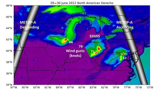
Summary composite image of the June 2012 North American Derecho displaying the 29 June descending node and 30 June ascending node METOP-A orbit (nadir) tracks, radar reflectivity (dBZ), and significant wind reports (kt) over (a) eastern CONUS and (b) the Mid-Atlantic region; NEXRAD radial velocity (kt) and significant wind reports (kt) over (c) eastern CONUS and (d) the Mid-Atlantic region along the storm track. Black oval outlines the derecho genesis region over the upper Mississippi Valley. Red circle in (a,c) marks the IASI retrieval location over Tipton, Iowa (“RTP”); (b,d) marks the IASI retrieval location near Salisbury, Maryland (“SBY”).
Figure 3.
Summary composite image of the June 2012 North American Derecho displaying the 29 June descending node and 30 June ascending node METOP-A orbit (nadir) tracks, radar reflectivity (dBZ), and significant wind reports (kt) over (a) eastern CONUS and (b) the Mid-Atlantic region; NEXRAD radial velocity (kt) and significant wind reports (kt) over (c) eastern CONUS and (d) the Mid-Atlantic region along the storm track. Black oval outlines the derecho genesis region over the upper Mississippi Valley. Red circle in (a,c) marks the IASI retrieval location over Tipton, Iowa (“RTP”); (b,d) marks the IASI retrieval location near Salisbury, Maryland (“SBY”).

Figure 4.
Hovmӧller diagrams of equivalent potential temperature (θe), with overlying plots of θe lapse rate (LR), in degrees Kelvin (K), derived from MWRPs at (a) Cedar Falls, Iowa, (b) Cleveland, Ohio, (c) Germantown, Maryland, and (d) Beltsville, Maryland, for the period 1200 UTC 29 June 2012 to 0400 UTC 30 June 2012. Dashed rectangles in (a–c) outline diagram extent in Section 3.

Figure 5.
(a) Davenport, Iowa RAOB sounding profile at 1200 UTC, (b) ground-based sounding profile retrieval from the Cedar Falls, Iowa microwave radiometer (MWR) at 1300 UTC, (c) METOP-A IASI sounding profile retrieved near Tipton, Iowa, at 1623 UTC, and (d) sounding profile retrieval from the Cedar Falls MWR at 1623 UTC 29 June 2012. Red curves and green curves represent the temperature and dewpoint soundings in degrees Celsius (°C), respectively. “MUCAPE” is most unstable parcel CAPE in J kg−1, “MWPI” represents the Microburst Windspeed Potential Index (Pryor 2015), “WGP” represents wind gust potential derived from the MWPI in knots (kt), “CI” represents conditional instability, and “PI” represents potential instability. ΓT and Γw represent dry-bulb temperature and wet-bulb temperature lapse rates, respectively.

Figure 6.
Velocity azimuth display (VAD) wind profile (VWP) in knots (kt) from (a) Davenport, Iowa NEXRAD between 1145 and 1230 UTC and (b) Chicago (Romeoville), Illinois NEXRAD between 1545 and 1630 UTC 29 June 2012. Black vertical dashed lines mark the radiosonde observation (RAOB) time at Davenport in (a) and the METOP-A MHS retrieval time in (b) as shown in Figure 5. “UC” represents the undercurrent in (b).

Figure 7.
NEXRAD reflectivity (dBZ) map-view images at 1400 UTC 29 June 2012 from (a) Des Moines and (b) Davenport, Iowa; 1300 to 1430 UTC 29 June 2012 Hovmӧller diagrams of (c) liquid density (g m−3) and (d) equivalent potential temperature (θe in degrees Kelvin (K)) as derived from Cedar Falls, Iowa MWRP. Des Moines NEXRAD DVIL is plotted over the diagrams at corresponding MWRP retrieval times.

Figure 8.
METOP-A MHS (a) 89 GHz channel brightness temperature (TB, degrees Kelvin (K)) image and (b) 157 GHz scattering index (SI157) at 1623 UTC 29 June 2012. (c,d) as in (a,b) with overlying Davenport, Iowa (DVN) NEXRAD reflectivity (dBZ) measurements. “CF” marks the location of the Cedar Falls, Iowa MWRP, “RTP”is the location of the IASI retrieval over Tipton, Iowa, and “53” is the location of the first severe wind report of the event (27 m s−1 (53 kt)) recorded at Burns Harbor, Indiana. White lines mark the 29 June descending node METOP-A orbit (nadir) tracks.

Figure 9.
Ground-based sounding profile retrievals from the Cleveland, Ohio, microwave radiometer (MWR) on 29 June 2012: (a) zenith at 2100 UTC, (b) south scan at 2100 UTC, (c) zenith at 2200 UTC, and (d) south scan at 2200 UTC. Red curves and green curves represent the temperature and dewpoint soundings in degrees Celsius (°C), respectively. “MUCAPE” is most unstable parcel CAPE in J kg−1, “MWPI” represents the Microburst Windspeed Potential Index (Pryor 2015), “WGP” represents wind gust potential derived from the MWPI in knots (kt), and “EML” represents the elevated mixed layer. ΓT and Γw represent dry-bulb temperature and wet-bulb temperature lapse rates, respectively.

Figure 10.
NEXRAD reflectivity map-view images from (a) Cleveland, Ohio (CLE), at 2232 UTC, (b) Detroit, Michigan (DTX), at 2230 UTC, and (c) Pittsburgh, Pennsylvania (PBZ), at 2230 UTC 29 June 2012.
Figure 10.
NEXRAD reflectivity map-view images from (a) Cleveland, Ohio (CLE), at 2232 UTC, (b) Detroit, Michigan (DTX), at 2230 UTC, and (c) Pittsburgh, Pennsylvania (PBZ), at 2230 UTC 29 June 2012.

Figure 11.
F-17 SSMIS (a) polarization corrected temperature (PCT) and (b) 150 GHz scattering index (SI150), in degrees Kelvin (K), at 2207 UTC 29 June 2012. (c,d) display the product imagery with overlying Pittsburgh, Pennsylvania NEXRAD reflectivity (dBZ). White circle marks the location of the Cleveland, Ohio MWRP. “DTX” and “PBZ” mark the location of the Detroit, Michigan, and Pittsburgh NEXRAD stations, respectively.

Figure 12.
2000 to 2315 UTC 29 June 2012 Hovmӧller diagrams of (a) liquid density (g m−3), (b) equivalent potential temperature (θe in degrees Kelvin (K)), and (d) vertical gradient of potential temperature (Del θ) as derived from Cleveland, Ohio MWRP. (c) Del θ Hovmӧller diagram (c) from 1200 UTC 29 June to 0400 UTC 30 June 2012 and (d) from 2000 to 2315 UTC 29 June 2012. Detroit, Michigan NEXRAD DVIL is plotted over (a) and (b) at corresponding MWRP retrieval times.

Figure 13.
METOP-A IASI retrievals near Salisbury, Maryland, during the evening of 29 June 2012 (0203 UTC 30 June): (a) IR+MW sounding profile; (b) IR+MW sounding profile modified by observed surface temperature and dew point at Salisbury Regional Airport; (c) modified IR+MW sounding profile plotted with virtual temperature. Red curves and green curves represent the temperature and dewpoint soundings in degrees Celsius (°C), respectively. “MUCAPE” is most unstable parcel CAPE in J kg−1, “MWPI” represents the Microburst Windspeed Potential Index (Pryor 2015), “WGP” represents wind gust potential derived from the MWPI in knots (kt), and “TPW” represents total precipitable water in inches (in). ΓT and Γw represent dry-bulb temperature and wet-bulb temperature lapse rates, respectively.

Figure 14.
(a) Modified METOP-A IASI IR+MW sounding profile retrieved near Salisbury, Maryland, at 0203 UTC 30 June 2012 as compared to (b) a ground-based sounding profile retrieval from the Germantown, Maryland, microwave radiometer (MWR). Red curves and green curves represent the temperature and dewpoint soundings in degrees Celsius (°C), respectively. “MUCAPE” is most unstable parcel CAPE in J kg−1, “MWPI” represents the Microburst Windspeed Potential Index (Pryor 2015), “WGP” represents wind gust potential derived from the MWPI in knots (kt), and “TPW” represents total precipitable water in inches (in). ΓT and Γw represent dry-bulb temperature and wet-bulb temperature lapse rates, respectively.

Figure 15.
(a) Modified METOP-A IASI IR+MW sounding profile retrieved near Salisbury, Maryland, at 0203 UTC 30 June 2012 as compared to (b) a ground-based sounding profile retrieval from the Howard University, Beltsville, Maryland (HUBC), microwave radiometer (MWR). Red curves and green curves represent the temperature and dewpoint soundings in degrees Celsius (°C), respectively. “MUCAPE” is most unstable parcel CAPE in J kg−1, “MWPI” represents the Microburst Windspeed Potential Index (Pryor 2015), “WGP” represents wind gust potential derived from the MWPI in knots (kt), and “TPW” represents total precipitable water in inches (in). ΓT and Γw represent dry-bulb temperature and wet-bulb temperature lapse rates, respectively.

Figure 16.
METOP-A MHS 89 GHz brightness temperature (TB, K) image at 0200 UTC 30 June 2012 with (a) overlying Sterling, Virginia (LWX) NEXRAD radial velocity (kt) and (b) reflectivity (dBZ) measurements. (c,d) as in (a,b) with overlying Sterling, Virginia (LWX) NEXRAD reflectivity (dBZ) measurements. “GER” and “BLT” mark the location of the Germantown and Beltsville, Maryland MWRPs, respectively. The white circle marks the location of the IASI retrieval over Salisbury, Maryland, and “62” is the location of the first severe wind report in the Washington, DC, metropolitan area (31.7 m s−1 (62 kt)) recorded at Dulles International Airport, Virginia. White lines mark the 30 June ascending node METOP-A orbit (nadir) tracks.

Figure 17.
(a,b) Sterling, Virginia NEXRAD Constant Altitude—Plan Position Indicator (CAPPI) reflectivity (dBZ) at 300 and 2500 m altitude, respectively, at 0235 UTC 30 June 2012; (c) 0144 to 0244 UTC 30 June 2012 Hovmӧller diagram of the deviation of equivalent potential temperature (in degrees Kelvin (K)) as derived from Germantown, Maryland MWRP.

Figure 18.
0200 to 0400 UTC 30 June 2012 Hovmӧller diagrams of (a) liquid density (g m−3) and (b) equivalent potential temperature (θe in degrees Kelvin (K)) as derived from Germantown, Maryland MWRP. Sterling, Virginia NEXRAD DVIL is plotted over the diagrams at corresponding MWRP retrieval times.
Figure 18.
0200 to 0400 UTC 30 June 2012 Hovmӧller diagrams of (a) liquid density (g m−3) and (b) equivalent potential temperature (θe in degrees Kelvin (K)) as derived from Germantown, Maryland MWRP. Sterling, Virginia NEXRAD DVIL is plotted over the diagrams at corresponding MWRP retrieval times.

Figure 19.
Velocity azimuth display (VAD) wind profile (VWP) in knots (kt) from Sterling, Virginia NEXRAD between 0200 and 0300 UTC 30 June 2012.
Figure 19.
Velocity azimuth display (VAD) wind profile (VWP) in knots (kt) from Sterling, Virginia NEXRAD between 0200 and 0300 UTC 30 June 2012.

Figure 20.
(a) TERRA MODIS split window IR brightness temperature difference product image at 0305 UTC 30 June 2012 compared to VAD wind profiles, in knots (kt), from (b) Sterling, Virginia, (c) Philadelphia, Pennsylvania (Manchester Township, New Jersey), and (d) Norfolk-Richmond, Virginia (Wakefield, Virginia) NEXRAD stations, surrounding the retrieval time of the MODIS image.


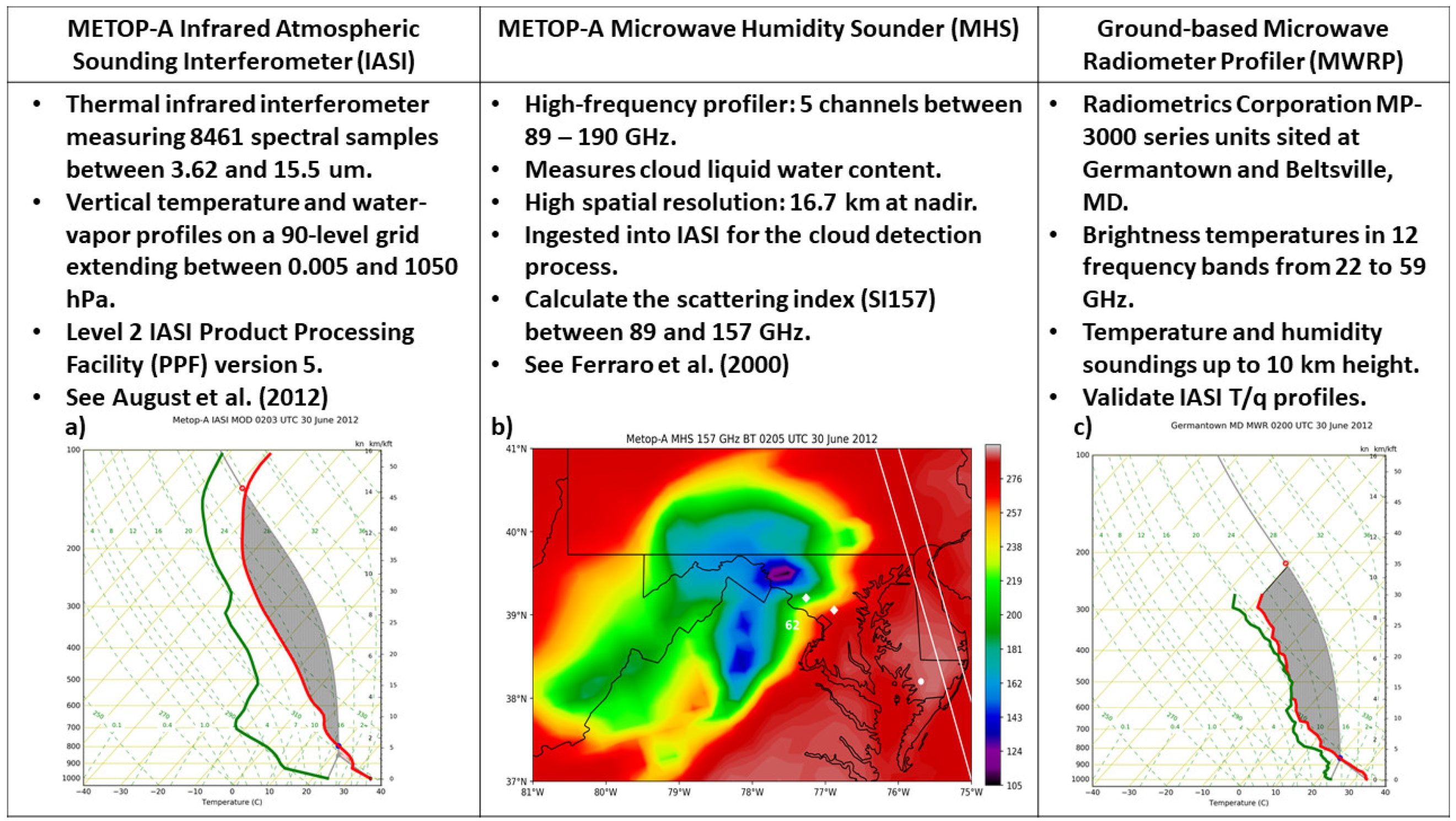
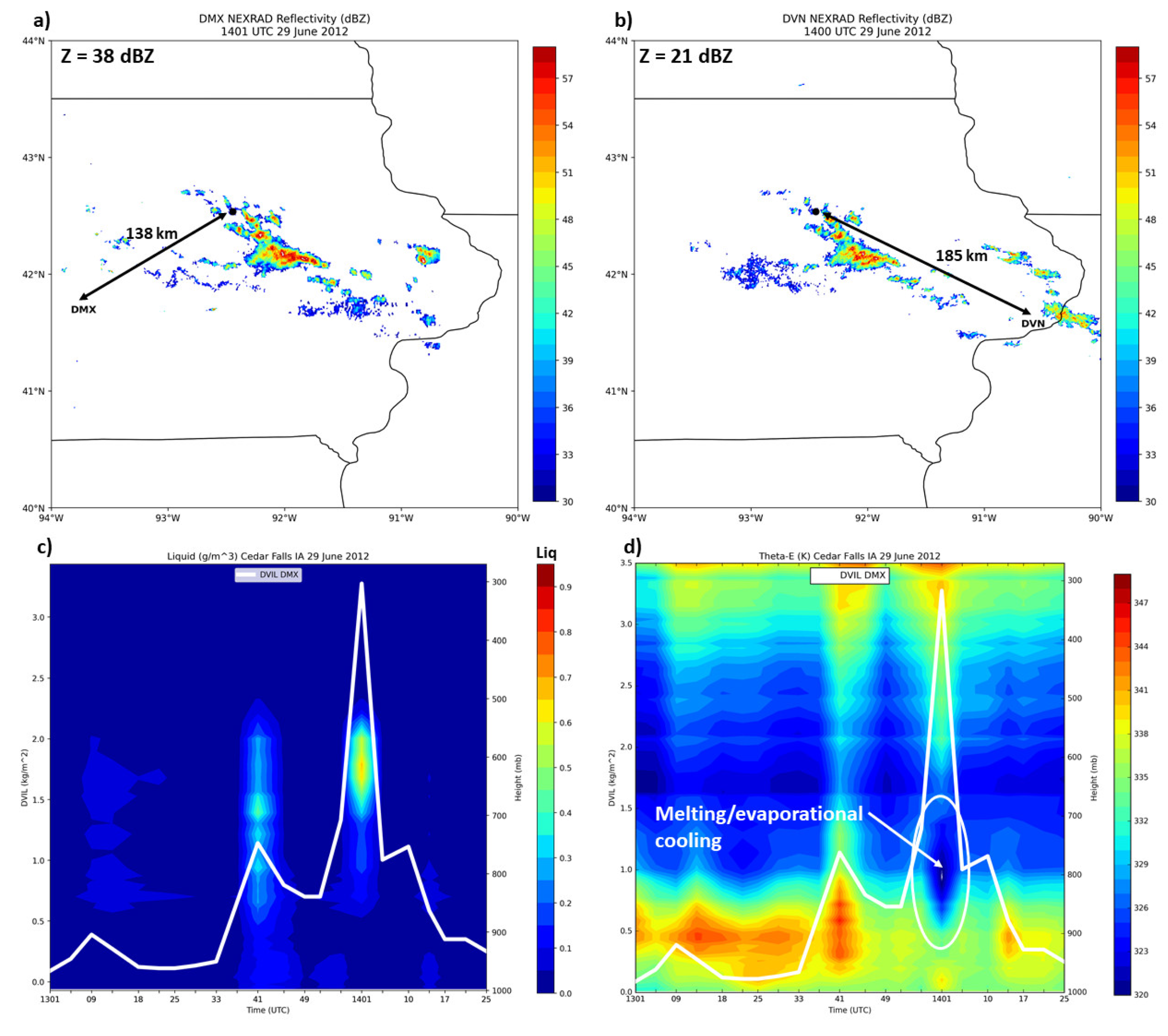
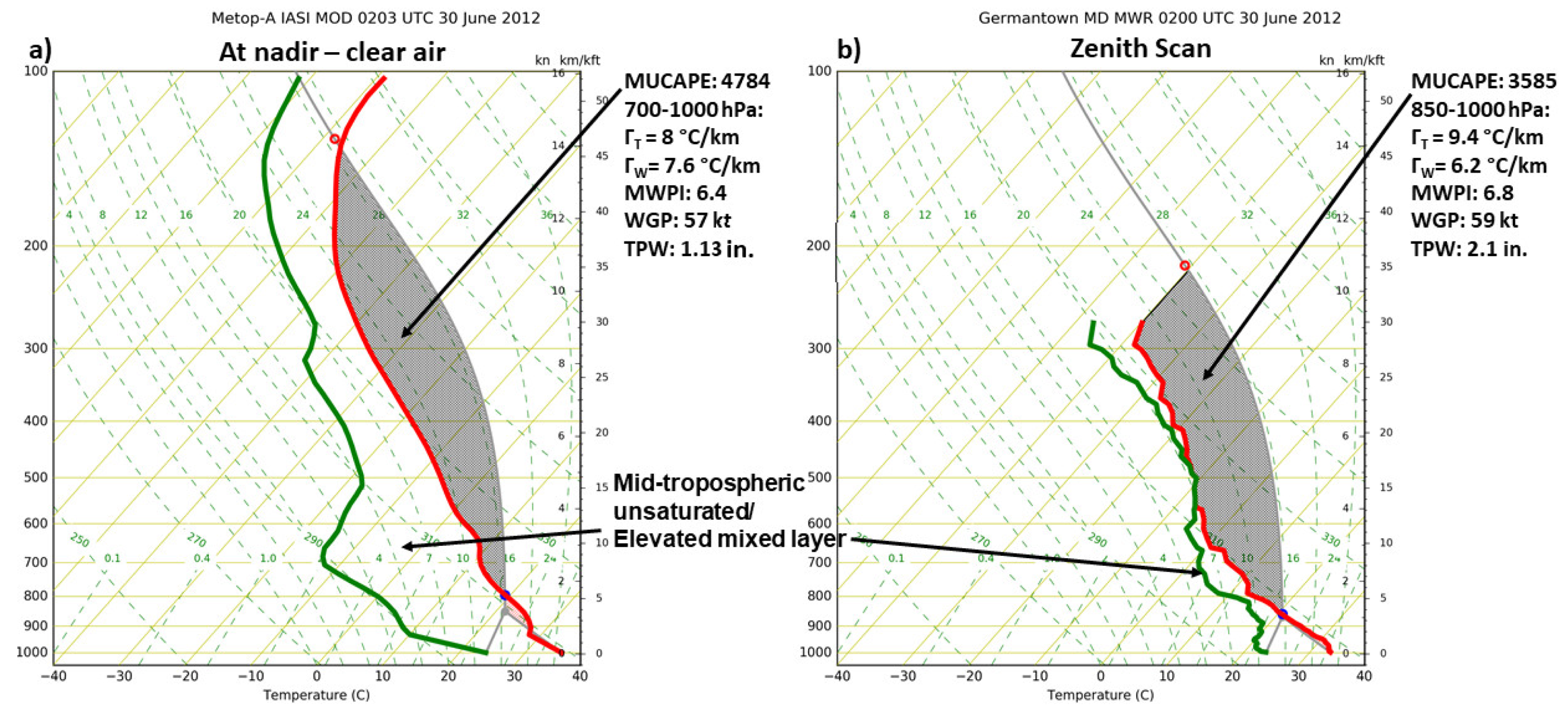
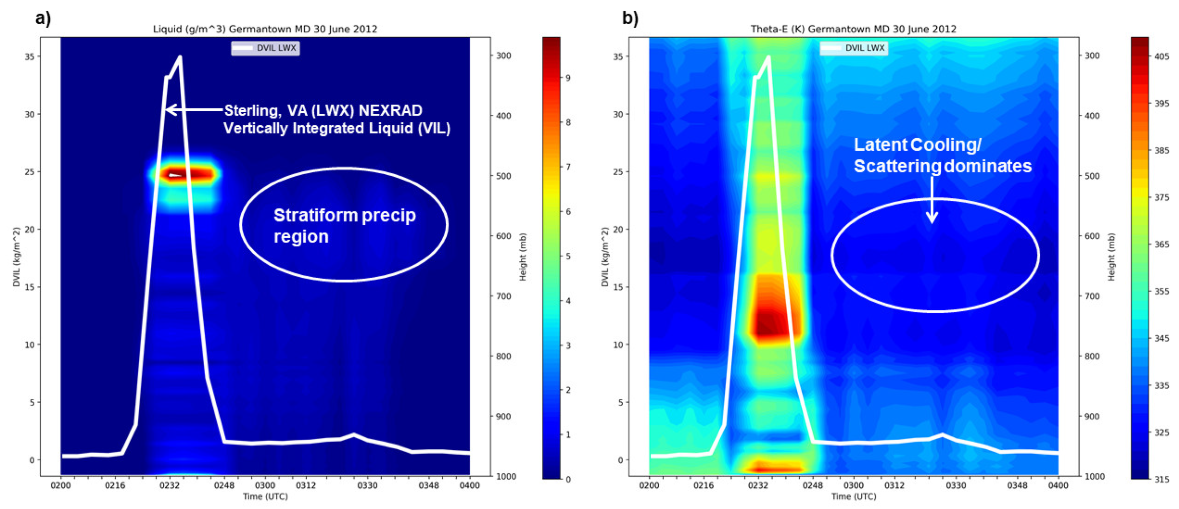
Table 1.
Derecho peak wind measurements (m s−1) compared to gust factors (G), surface peak temperature departures (ΔT), and MWR and IASI-derived MWPI values and associated wind gust potential (kt). Time is in UTC, ΔT in K, and wind gust potential (WGP) is in m s−1. “NA” denotes that an IASI retrieval not available at the event time.
| METAR Station | Date/ Time | Peak Wind | G | ΔT | MWR MWPI | MWR WGP | IASI MWPI | IASI WGP | Ret Time |
|---|---|---|---|---|---|---|---|---|---|
| DPA | 29/1602 | 23.7 | 2.42 | −5 | 4.8 | 24.7 | 3.8 | 22.6 | 1623 |
| MFD | 29/2136 | 19 | 1.85 | −8 | 1.9 | 19.5 | NA | NA | 2100 |
| IAD | 30/0235 | 30.4 | 2.27 | −9 | 6.8 | 30.4 | 6.4 | 29.3 | 0200 |
| DCA | 30/0252 | 31.4 | 2.54 | −10 | 6.8 | 30.4 | 6.4 | 29.3 | 0200 |
| BWI | 30/0305 | 29.3 | 1.78 | −10 | 6 | 28.3 | 6.4 | 29.3 | 0200 |
Table 2.
Correlation of peak wind and ΔT to MWR-derived MWPI values, and peak wind to ΔT.
| Peak Wind to MWPI | ΔT to MWPI | Peak Wind to ΔT | |
|---|---|---|---|
| R | 0.98 | 0.52 | 0.68 |
| R2 | 0.96 | 0.27 | 0.46 |
Publisher’s Note: MDPI stays neutral with regard to jurisdictional claims in published maps and institutional affiliations. |
© 2022 by the authors. Licensee MDPI, Basel, Switzerland. This article is an open access article distributed under the terms and conditions of the Creative Commons Attribution (CC BY) license (https://creativecommons.org/licenses/by/4.0/).
Share and Cite
MDPI and ACS Style
Pryor, K.; Demoz, B. A Retrospective Satellite Analysis of the June 2012 North American Derecho. Remote Sens. 2022, 14, 3479. https://doi.org/10.3390/rs14143479
AMA Style
Pryor K, Demoz B. A Retrospective Satellite Analysis of the June 2012 North American Derecho. Remote Sensing. 2022; 14(14):3479. https://doi.org/10.3390/rs14143479
Chicago/Turabian StylePryor, Kenneth, and Belay Demoz. 2022. "A Retrospective Satellite Analysis of the June 2012 North American Derecho" Remote Sensing 14, no. 14: 3479. https://doi.org/10.3390/rs14143479
Note that from the first issue of 2016, this journal uses article numbers instead of page numbers. See further details here.