
Airborne GNSS Reflectometry for Water Body Detection


1
Laboratoire d’Informatique, Signal et Image de la Côte d’Opale (LISIC), Université du Littoral Côte d’Opale (ULCO), 62228 Calais, France
2
National Council of Scientific Research (CNRS-L), Remote Sensing Research Center, Mansouriyeh 22411, Lebanon
3
School of Engineering, Lebanese International University (LIU), Beirut 14404, Lebanon
*
Author to whom correspondence should be addressed.
Remote Sens. 2022, 14(1), 163; https://doi.org/10.3390/rs14010163
Submission received: 1 December 2021
/
Revised: 25 December 2021
/
Accepted: 27 December 2021
/
Published: 31 December 2021
(This article belongs to the Special Issue Advances on Radar Scattering of Terrain and Applications)
Abstract
:This article is dedicated to the study of airborne GNSS-R signal processing techniques for water body detection and edge localization using a low-altitude airborne carrier with high rate reflectivity measurements. A GNSS-R setup on-board a carrier with reduced size and weight was developed for this application. We develop a radar technique for automatic GNSS signal segmentation in order to differentiate in-land water body surfaces based on the reflectivity measurements associated to different areas of reflection. Such measurements are derived from the GNSS signal amplitudes. We adapt a transitional model to characterize the changes in the measurements of the reflected GNSS signals from one area to another. We propose an on-line/off-line change detection algorithm for GNSS signal segmentation. A real flight experimentation took place in the context of this work obtaining reflections from different surfaces and landforms. We show, using the airborne GNSS measurements obtained, that the proposed radar technique detects in-land water body surfaces along the flight trajectory with high temporal (50 Hz ) and spatial resolution (order of 10 to 100 m). We also show that we can localize the edges of the detected water body surfaces at meter accuracy.
1. Introduction
Soil moisture is one of the key parameters in the hydrological cycle, i.e., the continuous circulation of water between oceans, atmosphere and land in a neverending process [1,2]. It directly influences the amount of evaporation, infiltration, and the amount of water uptake by plants, and was recognized as an Essential Climate Variable (ECV) [3,4]. In this context, measuring the soil moisture content can be of a great benefit in a large number of applications. Disciplines such as hydrology, climatology, and agriculture, require estimating the soil moisture content for prediction of potential flood and drought hazards, understanding land–atmosphere energy balance, and crop yield expectation [5,6]. The study of soil moisture content can be applied to observe the distribution of in-land water body surfaces.
Floodplains and in-land water body surfaces cover at least km (8%) of landscapes on Earth [7,8]. They play a significant role in the water cycle through river flow variability, flood mitigation, groundwater recharge and water quality improvement [9]. Despite its important role, little knowledge has been acquired concerning the water stored in floodplains and wetlands as well as its temporal variations from regional to global scales until remote sensing techniques emerged as potential instruments for soil moisture and water body detection. In this regard, soil moisture and water content remote sensing on a global and regional scale has been an active area of research over the past few decades. It has been proven that the microwave band that is optimal for soil moisture remote sensing lies within the L-band [10]. It is shown that the soil dielectric constant value that governs the surface reflectivity can be determined from only the top 0–5 cm of soil [10].
Global Navigation Satellite Systems-Reflectometry (GNSS-R) is an emerging bistatic remote sensing technique that uses the GNSS signals (mainly GPS signals) as sources of opportunity to characterize Earth surface. GNSS systems continuously transmit signals to Earth surface at different L-bands ranging between 1 and 2 GHz. A GNSS-R sensor receives the direct GNSS signals from the satellites as well as those reflected from the Earth’s surface. The reflected signals carry information about the reflecting surface, such as its height, shape, and moisture content. The reflecting surface can be an ocean, in which case, the sea level altimetry [11,12], wind speed [13,14], and ocean salinity [15] can be estimated, or land for studying the cryosphere including snow depth estimation [16,17] and sea ice detection [18,19], or for estimating the soil moisture content [10,20] and vegetation biomass [21].
GNSS-R platforms offer dedicated applications for Earth surface remote sensing on a local scale using ground-based experiments, a regional scale using airborne campaigns, and recently extending to a global scale using GNSS-R based spaceborne missions. Ground-based experiments have been proposed to prove the GNSS-R sensitivity to soil moisture [22,23,24,25,26,27,28,29]. Many studies have employed information on multipath effects from ground-based GNSS receivers to retrieve soil moisture content and biomass content sensing [24,25]. In [23,28], the Interference Pattern Technique (IPT) was employed to estimate the soil moisture content. The literature in [27] conducted the LEiMON experiment, a ground-based experimental campaign that is based on continuous polarimetric measurements of GNSS scattered signals in order to improve the accuracy of the reflectivity measurements.
Several airborne campaigns have shown the feasibility of retrieving soil moisture using reflected GNSS signals [5,10,30,31,32,33,34,35,36]. Masters et al. [5] conducted an airborne soil moisture remote sensing experiment in order to extract the soil moisture content from the measurements of the surface reflectivity by deriving the relation between the power of the GNSS signals, the Fresnel coefficient, and the soil moisture content. In 2016, Motte et al. [36] introduced the GLObal navigation satellite system Reflectometry Instrument (GLORI), dedicated to the study of land surfaces (soil moisture, vegetation water content, forest biomass) and in-land water bodies from airborne flights. This instrument used two hemispherical GPS dual-frequency (L1 and L2) dual-polarization active antennas and mainly relied on Delay Doppler Maps (DDM) with a total integration time of 1 s to obtain measurements of surface reflectivity. At the beginning of 2021, a study [31] performed a comparison of two different data sets acquired with the Microwave Interferometer Reflectometer (MIR), an airborne-based dual-band (L1/E1 and L5/E5a), multiconstellation (GPS and Galileo) GNSS-R instrument. In this work, the effective integration time was set to 5 s to neglect surface roughness effects. The use of such integration time led to a decrease in the spatial resolution of the application.
Few studies [7,37,38] have been conducted concerning the detection of in-land water body surfaces using airborne GNSS-R techniques. These studies also lacked quantitative analysis concerning the localization accuracy of the detected water body surfaces and the detection capacity of the proposed techniques over large flight trajectories and mostly recurred to very few number of test areas. In 2015, Troglia et al. [37] developed a GNSS-based sensor for UAVs and small manned aircraft, used to classify lands according to their water content. The classification is based on the Signal-to-Noise (SNR) ratio between the direct and reflected signals. This experiment used a dual antenna configuration with one up-looking and two down-looking antennas. The sensitivity of the approach was tested on an in-land water body surface. Its main limitations arise from (1) the use of different components in the receiving channels, leading to power and phase variations between the LHCP and RHCP channels, and (2) the instrument antennas, which are affected by cross-polarization isolation issues, thus preventing reliable polarimetric measurements.
Most recently, exhaustive demonstration of the sensitivity of spaceborne reflected GPS signals to changes in the soil moisture has been carried out using data from TechDemoSat-1 (TDS-1) [39,40] and data from the Cyclone GNSS (CYGNSS) missions [41,42]. GNSS-R spaceborne missions promise enhanced resolution compared to passive satellite missions for soil moisture remote sensing. Currently, there are two L-band passive microwave spaceborne missions specifically devoted to measuring soil moisture: the Soil Moisture and Ocean Salinity mission (SMOS) and the Soil Moisture Active and Passive mission (SMAP). Both SMOS and SMAP derive global maps of soil moisture from brightness temperature measurements at a spatial resolution of 35 to 36 km with a 3-day revisit time. On the other hand, CYGNSS provides observation of soil moisture at a spatial resolution of ∼500 m determined by the major-axis size of the first Fresnel zone for flat surfaces with coherent bistatic scattering and up to ∼10 km for rough surfaces with incoherent (diffuse) bistatic scattering [43]. The CYGNSS constellation consists of 8 observatories in order to provide measurements as frequently as possible. This results in a mean revisit time of 6 to 7 h. The primary GNSS-R spaceborne missions employ conventional GNSS-R (cGNSS-R) signal proccessing techniques to obtain DDM observables, which is the basic product containing physical information of a surface. In this regard, CYGNSS satellites generate on-board DDM products with an integration time of 1 s.
However, GNSS-R spaceborne missions still suffer from a relatively low spatial and temporal resolution compared to ground-based and airborne experiments. The spatial and temporal resolution of such GNSS-R applications depend on the receiver height as well as the constraints and requirements of the application. A minimal height implies a maximized spatial resolution but with less coverage. In this regard, there is a trade-off between spatial resolution and global coverage. The maximum temporal resolution of GNSS-R ground-based and airborne applications is equivalent to the code repetition rate of GNSS signals (e.g., 1 ms for GPS C/A). However, a longer integration time increases the Signal-to-Noise (SNR) ratio of the signal, which is important when studying land reflections due to the weak nature of the reflected signals.
This article is dedicated to the study of airborne GNSS-R techniques for water body detection using a low-altitude airborne carrier with high rate reflectivity measurements. We develop a radar technique for automatic GNSS signal segmentation in order to differentiate surfaces, and in particular water bodies, in landforms based on the changes in the reflectivity measurements associated to different areas of reflection. Such measurements are derived from the GNSS signal amplitudes. We have shown in a previous work [44] that in a 1-bit quantization digital receiver, the digitized GNSS signals are independent of the automatic gain control and thus dedicated GNSS signal processing techniques provide direct observation of the GNSS signal amplitude. In the context of this work, we estimate 20 ms rate of the GNSS signals amplitudes using 20 ms rate observations of the signals components. We estimate high rate (50 Hz rate) reflectivity measurements in order to cope with the rapid displacement of the satellites footprints along the airborne experiment. We propose a mixture of an on-line/off-line change point detection and localization algorithm for the segmentation of the GNSS signals into stationary parts associated to different mean signal levels. We develop a GNSS-R setup on-board a lightweight airborne carrier that can achieve the high temporal and spatial resolution requirements of our application. We show, along a real flight experimentation, that the proposed radar technique detects in-land water body surfaces along the flight trajectory. We also show that we can localize, at meter accuracy, the edges of the detected water body surfaces, i.e., the border between water and land.
Based on the foregoing, this chapter is organized as follows: Section 2 describes the airborne bi-static GNSS-R configuration. Section 3 introduces the airborne GNSS-R system that we utilize in this work. Section 4 demonstrates the on-line/off-line change model that is proposed for GNSS signal segmentation. In Section 5, we introduce the context of the real flight experimentation. Analyses of the data acquired during the flight for water body detection and edge localization are provided in Section 6. Discussion and conclusions are provided in the final two sections.
2. Airborne Bi-Static GNSS-R Configuration
GNSS-R consists of using GNSS signals received on Earth directly from the GNSS satellites as well as after a reflection on the Earth’s surface. In our implementation, we use a GNSS-R dual antenna geometry. The direct GNSS signals are received by a Right Hand Circular Polarized (RHCP) antenna, and the reflected GNSS signals are received by a Left Hand Circular Polarized (LHCP) antenna after specular scattering from different landforms along the flight trajectory as shown in Figure 1. Once a signal hits a reflection point on Earth, scattering occurs primarily from the region of the surface surrounding the specular reflection point.
On flat areas with no topography, the specularly reflected power can be derived solely from the Fresnel reflection coefficients. In this case, the spatial resolution of the GNSS measurements is mostly linked to the size of the first Fresnel zone which in turn determines the surface reflectivity. In this work, we process the amplitudes of the RHCP and LHCP antenna signals in order to measure the reflectivity of the surface. The reflectivity measurements are defined as the ratio of the amplitudes of the reflected LHCP antenna signals over the amplitudes of the direct RHCP antenna signals as shown below:
We associate these measurements with 20 ms rate specular point localization.
3. Airborne GNSS-R System
We present in Figure 2 the GNSS-R system used in our airborne experimentation. The GNSS-R setup developed for this application consists of a typical GNSS-R sensor that uses an RHCP antenna and an LHCP antenna with a single mono-channel bit grabber for signal digitization. A delay line is used to separate the RHCP antenna signals and the LHCP antenna signals in time so that both signals can be tracked independently using a mono channel receiver with perfect phase and frequency synchronization. The specular points are localized as a function of the GPS time with the use of RINEX files and on-board drone card measurements. The raw data recorded by the GNSS-R receiver correspond to the samples of the direct and reflected GNSS signals at the output of the antennas (after frequency down conversion).
After collecting the raw GNSS data, dedicated GNSS signal processing techniques are implemented in our self-built GNSS software receiver for the extraction of the required GNSS data. The processing of the GNSS signals adapts a master/slave configuration. The direct signals processing can be derived from the classical GNSS demultiplexing and demodulation processes in the form of Phase Lock Loop (PLL), Frequency Lock Loop (FLL), and Delay Lock Loop (DLL) to obtain the corresponding GNSS data. The estimated code and frequency delay of the direct signals are used in the model aided tracking of the reflected GNSS signals. As a result, GNSS observations related to the direct and reflected signals (i.e., in-phase component of the signals, code delay, frequency delay and phase delay estimates) are derived. The message of navigation is extracted in the process and the GPS time of each data is derived after signal dating.
The GNSS data provided by the direct and reflected signals tracking loops are used in order to obtain observations of the GNSS signals amplitudes. Then, the reflectivity measurements are derived from the amplitudes of the GNSS signals as a function of the GPS time. The GNSS signals are segmented into stationary parts based on the changes in reflectivity using the segmentation model developed in this work. These segments are associated with different areas of reflections represented by the specular point localization. For this purpose, the specular point coordinates and the segmented GNSS signals are linked using the GPS time provided by on-board sensors and the GPS time extracted from the digitized GNSS signals.
4. Segmentation of the GNSS Signal
4.1. Transition Model
In our radar application, the amplitude of the reflected GNSS signal changes as a function of time. The GNSS signal amplitude is proportional to the ground reflectivity contained in the surface of the first Fresnel zone of the satellite footprint. The first Fresnel zone is an ellipse centered on the specular reflection point. The displacement of this ellipse on the ground follows the satellite trace. We show in Figure 3, the satellite footprints displacement from one area to another. We show in Figure 4 the signal model in the working window.
We can observe in Figure 4 that when the mean value of the GNSS signal amplitude is equal to , the ellipse is on the first area (land), and when the mean value of the GNSS signal amplitude is equal to , the ellipse is on the second area (water body). We observe that at the border between different areas of reflection, the change in the signal level is not abrupt but rather transitional. That is why a transition model is adapted to characterize the changes in the amplitudes of the reflected GNSS signals. We assume that the GNSS measurements are piecewise stationary and the noise on the observations are additive, Gaussian and centered. The increasing evolution of the signal model between the mean values and in Figure 4 models a linear transition from a surface of low reflectivity (land) to a surface of higher reflectivity (water body). We define in Section 4.3 the start and end instants of the working window in order to optimize the estimation.
In the presence of a large amount of data that need to be processed, an on-line change detection process needs to be implemented. In this regard, we use the CUSUM algorithm [45,46,47] to detect a change on-line. The CUSUM change detector is capable of detecting changes associated to the model of transition that we use in this work. After the changes are detected on-line, an off-line localization approach is proposed to localize the detected change points. We propose a maximum likelehood estimate for change localization. This approach is close to the optimal estimation because we maximize in this case the size of the working window in which the detected change point is localized.
4.2. Change Detection
We show in Figure 5 the architecture of the change point detector. The amplitudes of the direct and reflected GNSS signals are estimated with an Extended Kalman Filter (EKF) that uses the in-phase components of the signals as observations based on the model proposed in [44]. A Kalman filter and a CUSUM algorithm are used to detect a change at instant . l is the satellite and i is an instant of time. and are respectively the state and measurement vectors. represents the estimated GNSS signal amplitudes. is the innovation of the EKF and is the covariance of the innovation. When a change is detected an alarm is generated to initialize the Kalman filter.
We show in Figure 6 the GNSS signal amplitude and the filter innovation as a function of time. The CUSUM detection algorithm uses an integration of the innovation process in order to detect the changes in the GNSS measurements. At a transition of the signal, between two stationary pieces, the innovation increases and then decreases (or vice versa) to produce a peak. When a change occurs in the mean of the innovation, the mean value after the change is either or with , the dynamic of the change, assumed to be known. In this work we use a two-side CUSUM algorithm [47]. The CUSUM detection process is defined by
where and is the instant of change detected for satellite l. Before the change, the mean of the innovation process is , and and , the integration of the innovation process, evolves as a Gaussian random walk. After the change instant defined in Figure 4, and are monotonic increasing functions. In our implementation, we assume that the innovation before and after the change is distributed according to a Gaussian distribution notice where and are, respectively, the mean and the standard deviation of the distribution. The normalized innovation process is distributed according to before the change and after the change.
According to the transition model defined in Figure 4, the theoretical value of the detection threshold can be defined as with . In practice, is a parameter defined by the user. It represents the minimum change dynamic that we want to detect. In our application, , the length of the transition area in the change model, is defined with the satellite elevation angle, as well as the speed and height of the airborne carrier.
4.3. Change Localization
In this work, the dynamic of the change is not known. We propose an off-line Maximum Likelihood Localization Estimate (MLLE) for change point localization. We show in Figure 7 the architecture of the proposed change point estimate.
According to the signal model of Figure 4 and assuming that the noise is additive, white-centered, and Gaussian, we derive a maximum likelihood estimate of t, the starting instant of the transition and , the duration of the transition. The estimates are processed with the GNSS signal amplitudes observations in the working window . The GNSS amplitude observations are obtained from the in-phase observations [44]. is the localization of the change for satellite l and is the detected change instant provided by the CUSUM detector for satellite l. In the rest of the section, we will note as and as to simplify notations. N is the number of samples in the working window defined between , the previous localized change by MLLE and , the next detected change by CUSUM.
In practice, the CUSUM detector detects a change after its actual position, as shown in Figure 8a. In this case, the working window is not optimal, but nearly optimal with a difference of very small number of samples at the end of the window. This number of samples represents the difference between the detected and localized change point position at the instant .
To estimate the localized change instant , we define the likelihood function as:
and are the mean values of the GNSS signal amplitude before and after the change, respectively. is a sampling line that models the growth of the reflectivity from to defined between and . We can express the negative log likelihood as follows:
In practice, the parameters of the log likelihood function are estimated using empirical maximum likelihood estimation. The empirical variances are defined by:
We can derive the expression of the empirical maximum likelihood estimate of and by:
Finally, the empirical maximum likelihood estimate is given by:
In practice, the estimate value is searched in a working window of N samples defined between and . The estimate value is searched between and . The value of is dependent on the application. For our application to airborne GNSS-R data, is a function of the length of the major axis of the first Fresnel zone ellipse associated with the satellite footprint. According to the signal model, the true position of the border between two different areas which corresponds to the true change point position is assumed to be at as shown in Figure 8b. This position can be in practice the beginning or the end of the edge of a water body along the satellite footprint trace.
4.4. Segmentation of Airborne GNSS Measurements
We show in Figure 9 the reflectivity measurements obtained with our GNSS-R receiver embedded on a gyrocopter. The surface reflectivity increases with the water content of the soil. Figure 9 shows the changes in the signal reflectivity associated to the reflections from land and from water bodies. In order to detect and localize water bodies, we apply an automatic segmentation of the signal using the reflectivity measurements based on the change detection and localization algorithms presented in the previous sections. Firstly, the changes in the reflectivity of the GNSS signal are detected with the Kalman-CUSUM algorithm (Figure 9a). Then, these changes are localized using the proposed MLLE approach (Figure 9b). Finally, the signal is divided into different segments associated to different mean reflectivity levels based on the localized change positions (Figure 9c).
The results obtained in Figure 9 show the feasibility of our approach to segment a real reflectivity signal obtained in an airborne experiment. In this context, the proposed approach is used for the detection and localization of in-land water body surfaces. This evaluation is realized with signals of reflectivity obtained for different satellites along the trajectory. The airborne experiment is described in the next section.
5. Flight Experimentation
5.1. Flight Information
The flight took place in the North of France and started at 14:45 UTC, the 19 October 2020 and ended at 15:30 of the same day lasting for 45 min. We show in Figure 10 the gyrocopter that was used for the flight experimentation with the different sensors embedded on it. The gyrocopter (MTO Sport 2017) is a light aircraft with an approximate weight of 245 kg and size of 5.1 m × 1.9 m × 2.7 m. It can carry a load up to double its weight. The maximum speed that the gyrocopter can fly at is 195 km/hr. It can cover a distance up to 700 km with 6.7 h loft within a single flight.
An RHCP antenna is fixed on the nose of the gyrocopter pointing towards the zenith and an LHCP antenna is mounted on the bottom of the gyrocopter pointing towards the nadir. A drone board sensor records the receiver’s attitude, altitude and position with respect to the GPS time. In addition to the on-board sensors, the gyrocopter was loaded with the necessary setup that constitute the GNSS-R receiver hardware for data collection. This receiver is composed of a delay line, combiners/splitters and a Syntony L1-L5 bit grabber for digitizing the composite signal.
The gyrocopter took off from Calais–Dunkerque Airport located in Marck, 7 km east-northeast of Calais, in the Hauts-de-France region. We scanned a large zone that borders the English Channel over a trajectory of ∼71 km between Calais, Escalles, and Ardres. This study area was selected for experimentation because it contains a number of different landforms. The topography of the study area, especially the region between Guînes and Ardres, does not vary a lot as it only contains plain land, water bodies, and some forests with no landscapes that might hugely affect the topography of the surface (such as mountains or big hills). This specific region holds over 50 different water body surfaces (such as lakes, ponds, rivers, swamps, etc.) of different nature and sizes. The effects of the study area surface roughness on the reflectivity measurements are not taken into consideration since we aim for the detection and localization of in-land water body surfaces using the variations of the measurements as we obtain reflections from different landforms along the trajectory rather than its estimated value. The flight trajectory and study area are shown in Figure 11.
During the flight, the gyrocopter maintained a low altitude of approximately 315 m above the ground with an average speed of 95 km/h. The wind speed was approximately at 25 km/h. Table 1 presents an overview of the flight information.
5.2. Flight Trajectory
Figure 12 depicts the traces of the satellites footprints along the flight trajectory imposed on Google Earth software. The traces of very low elevation satellites are not shown in Figure 12. In our application, we aim to study reflections from satellites with high elevation angles in order to maximize the spatial resolution of our application. In this regard, we fix the maximum size of the major axis to 23 m, so the minimum satellite elevation to 50. An average of 9 GPS satellites have been detected along the trajectory. Three GPS satellite signals of elevation angles superior to 50 were extensively analyzed to observe the reflectivity of the different areas of reflections. These signals corresponds to satellite PRNs 5, 7, and 30.
Concerning the temporal resolution of the application, the raw data were sampled at a frequency of 25 MHz and the GNSS measurements are realized at a rate of 50 Hz. Taking into consideration the average speed of the gyrocopter (95 km/h), the distance between two consecutive specular points is approximately 0.5 m. This means that every 20 ms the footprints are displaced by 0.5 m. The size of the GNSS data that constitutes the sampled direct and reflected GNSS signals digitized and stored (in bytes format) by the Syntony bit grabber for GPS L1 signals is 133.78 GB.
We apply the GNSS signal segmentation in the next section for water body surface detection and edge localization.
6. Data Analysis
6.1. Radar Signal Segmentation
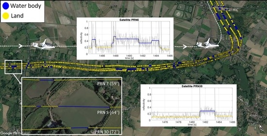
Figure 13 presents the GNSS measurements for an area located at (50.888515°N, 1.871803°E) along the trajectory. In the upper figure, the traces of the satellites footprints are represented by 20 ms rate localization of the specular points of reflection. The colors of the points represent different reflectivity measurements associated with different kinds of reflecting surfaces. The number in brackets notes the satellite elevation angle. On the lower figures, we show the GNSS reflectivity measurements and the automatic signal segmentation associated to it using our proposed radar technique over 12 s of data from this area.
We can notice from the graphs that a difference in the mean of the measurements separates different areas of reflection. We remark a significant increase in reflectivity corresponding to water body surfaces. This increase is not constant though and is dependent on the type of land and water that the signals are reflecting from. We can observe from the graphs of Figure 13 that the proposed radar technique detects different water bodies corresponding to different mean reflectivity levels shown in blue segments. These segments are associated with a blue coloring of the specular points on the Google Earth image. The yellow coloring of the specular points is associated to land reflections. We can also observe fluctuations in the mean reflectivity level (blue segments) corresponding to the detected swamp by satellite PRN 7. This is due to the trace of satellite PRN 7 passing through a small green area in the middle of the swamp that can be a very wet piece of land or small set of leaves that have been accumulated over time.
We show in Figure 14 different types of water bodies detected along the traces of the satellites footprints. We observe that the radar technique detects in-land water bodies with various sizes and shapes and under different environments. It is worth noting that the approximate size is not the same for all the surfaces of the same water body type. We notice that we detect large-size contained water body surfaces such as lakes (Figure 14a) and swamps (Figure 14b). We also differentiate smaller contained water body surfaces such as wetlands (Figure 14e). In our study, we differentiate lakes from ponds based on the size of the water body surface. We differentiate swamps from lakes and ponds based on the characteristics of the water body and the surrounding environment. However, this is not always explicit by manual inspection using Google Earth map imagery data.
Rivers of different widths along the trajectory are detected by the traces of all three satellites due to its length. The river shown in Figure 14c has a width of 21 m. We notice in Figure 14d, two small streams of 3.6 m and 5.76 m width, while we notice in Figure 14f that the proposed radar technique was able to detect a small pool of 4.5 m × 9 m size along the trace of satellite PRN 5 footprints. This shows the sensitivity of the proposed radar technique to changes in landforms and shows the importance of high spatio-temporal resolution in the detection of in-land water body surfaces using low-altitude airborne carrier.
6.2. Water Body Surface Detection
The proposed radar technique is first applied for detecting water body surfaces in landforms. We represent the specular points of reflection corresponding to the detected water body surfaces by our radar technique for the three satellites in study on maps provided by the French National Institute of Geographic and Forest Information (IGN) maps using QGIS software. IGN maps maintain geographical information for France managing geodesic and leveling networks, aerial photographs and geographical databases and maps. IGN maps provide up-to-date map schemes that clearly show the actual locations of the water body surfaces at the day of the experimentation. The aim is to assess the performance of the proposed method for water body surface detection. Figure 15 shows the detected water body surfaces using our proposed method for the area between Guînes and Ardres represented by a blue coloring of the specular points of reflection.
The proposed method detects water body surfaces whenever the reflectivity measurements are beyond a specified threshold. From the analysis of the GNSS measurements obtained, the reflectivity threshold used in this study is 0.21 for the three satellites. We compare the number of water body surfaces provided by IGN maps along the satellite footprints traces with the percentage of detections of these water bodies using our proposed approach. Table 2 details the results of the manual inspection applied between the IGN images and our radar technique for water body surface detection.
We show in Table 2 that our radar technique detects of in-land water body surfaces (i.e., 45 out of 47 surfaces) along the satellites footprint traces as compared to the details provided by IGN maps. We detect of large-size contained water body surfaces (i.e., lakes/large swamps) and of large waterways (such as rivers and canals). However, we miss one small-size contained water body surface and one stream along the trajectory. We cannot clearly observe the reason using maps such as IGN or Google Earth as it is not evident whether the miss is due to a detection inaccuracy or due to the water bodies being masked by vegetation (such as trees or groves).
Although IGN maps provide updated map imageries, we can observe from Figure 15 that these maps do not provide sufficient information about the water body characteristics (e.g., type, shape, and approximate size) nor the vegetation possibly covering it. Thus, we propose to use satellite images provided by Google Earth software for water body edge localization.
6.3. Water Body Edge Localization
The proposed radar technique is applied for localizing the edges of the detected water body surfaces along the satellites footprints traces. Google Earth does not provide up-to-date map images. In this regard, the Google Earth images and the experimentation were obtained with one year of difference (Google Earth dates its imagery data to September 2019). We select in our study the water body surfaces that can be clearly observed using both IGN maps and Google Earth. We can assume that the water level was the same between the 2 dates. We assess the accuracy of the proposed automatic edge localization technique using manual edge localization on Google Earth.
We report in Table 3 the parameters of the detected water body surfaces by satellite PRN 5 for 100 s of an area along the trajectory. We report the approximate size (in meters) for each of the mentioned surfaces. We also report the difference in localization between the automatic and manual approach (in meters) for the starting and ending edges of the detected water body surfaces. These values can be positive or negative. In addition, we record the total localization distance error (in meters), i.e., the total absolute offset for the start and end edges of each water body as well as the automatic and manual detection length (in meters), i.e., the length covered by the satellite footprints trace along the water body surface using the proposed radar technique and Google Earth, respectively.
We observe in Table 3, perfect edge localization (i.e., zero total distance error) for the lake by the proposed radar technique as compared to Google Earth. The localization of the river edges are less accurate especially for the start of the river but clearly better than that of wetland and stream. In this regard, edge localization requires precise measurements. The localization accuracy is affected by the characteristics of the water body surface (type, shape, size, etc.), as well as the nature of the landforms surrounding the water body at its edges. We can clearly observe from the Google Earth images that the stream reported in Table 3 is small in size (4.56 m width), muddy, and surrounded by vegetation. It is worth noting that this stream reported the lowest localization accuracy among all the water body surfaces localized along the traces of the three satellites footprints during the whole trajectory. Other streams are localized more accurately.
We apply the aforementioned quantitative analysis for the detected water body surfaces by the traces of the three satellites’ footprints along the whole trajectory. We report in Table 4 the number of detections of each water body type as well as the percentage of perfect edge localizations (i.e., whenever the total localization distance error is 0). We also record the mean distance localization error (in meters) which is the absolute value of the offset in meters between the manual and the automatic edge localization. Finally, we record the localization difference standard deviation (in meters) which represents the standard deviation of the difference in the starting and ending edges.
We can also observe in the histogram of Figure 16, a comparison of the number of perfect and imperfect localizations with respect to the total number of water body edge localizations per type. We notice from the second column of Table 4 and from Figure 16 that swamps had the highest localization accuracy with (26 perfect localizations out of 30) followed by lakes and rivers with an accuracy of for each with the same number of detections. The pool had the lowest edge localization accuracy with but from just 2 measurements. Streams/brooks noted the second lowest edge localization accuracy with from 12 localizations.
We note from Table 4 that swamps had the least mean localization error of 0.36 m and the lowest localization difference standard deviation of 0.5 m (after the pool). Although lakes and rivers have the same percentage of perfect edge localizations, we notice that the lakes had lower mean distance localization error and localization difference standard deviation, implying better overall localization accuracy for lakes. The oxbow lake and streams reported the highest statistical errors in terms of the recorded mean and std. We notice that the only oxbow lake detected along the trajectory was surrounded by vegetation on its borders. In addition, as previously discussed, the streams along the trajectory are mostly muddy and covered by trees. The results are in agreement with those derived in Table 3, but applied for the whole study area and for the three satellites. We can observe that the edge localization is affected by the type of the water body surface, as well as the characteristics of the landforms surrounding the water body at its edges (vegetation biomass, roughness, etc.).
In total, the proposed radar technique achieved an overall water body edge localization accuracy of with a mean distance localization error of 0.96 m and localization difference standard deviation of 0.9 m. From this study, we conclude that we can achieve the meter accuracy for water body edge localization with our automatic approach as compared to manual localization using Google Earth taking into consideration the spatial resolution of our GNSS-R application and the approximate distance between two consecutive specular points (∼0.5 m) for a gyrocopter average speed of ∼95 km/h.
7. Discussion
The accuracy of water body edge localization by the proposed radar technique is affected by the inaccuracies that Google Earth encounters while processing its map imagery. One of the main perspectives of this work is to compare the results obtained for water body detection and edge localization using the proposed radar technique with the ground-truth data. This requires extensive in situ measurement campaigns with the use of precise GNSS-R positioning techniques to accurately localize the starting and ending edges of the in-land water body surfaces. In order to better analyze the variations in the reflectivity of a water body surface, we aim to make use of real-time images captured by action cameras embedded on the bottom of the gyrocopter as part of the new GNSS-R receiver setup. This would also allow us to analyze the reason of possible misses in the detection of water body surfaces, as well as to track the number of false detections by the proposed radar technique as it is practically impossible using maps.
We have also seen from the analysis of the GNSS reflectivity measurements that it is exceptionally complicated to differentiate other surfaces in landforms such as plain land surfaces and groves. One of the interesting aspects of the mono channel bit grabber used in this work is the digitization of L1 and L5 signals. The next step in this direction would be the processing of L5 signals and the fusion of L1 and L5 data to further increase the observables of the reflected GNSS signals. An information fusion algorithm based on statistical approaches would be developed for the integration of the GPS L1 and L5 signals. The GPS L5 signals have higher transmitted power than L1 signals and they are expected to have deeper penetration capacity in land for more accurate reflectivity measurements, allowing more precise detection of other surfaces in landforms (other than in-land water bodies). In addition, for more accurate reflectivity measurements, the gain patterns of the antennas should be taken into account.
8. Conclusions
This airborne experiment studies the techniques for water body localization using GNSS-R. A GNSS-R setup of reduced size and weight was developed specifically to meet the requirements of this application. The utilization of the delay line in the GNSS-R setup is a significant contribution of this work. The delay line produces a delay that is sufficient enough to track the direct and reflected GNSS signals independently using a mono channel receiver which allows perfect synchronization of the RHCP and LHCP links. The observations are realized with high temporal and spatial resolution. We estimate the reflectivity measurements as the ratio of the amplitudes of the reflected LHCP antenna signals over the amplitudes of the direct RHCP antenna signals. The signals are segmented into stationary parts associated with different areas of reflection. We relate the 20 ms rate reflectivity measurements to the corresponding reflecting surfaces via a 20 ms localization of the specular points of reflection. We apply a real flight experimentation using a low-altitude airborne carrier with high rate observations of the surface reflectivity. We show that our method is able to differentiate surfaces, and thus detect water bodies in landforms, based on the difference in reflectivity measurements associated to each surface. We show that our radar technique is able to detect of the total number of water body surfaces on the traces of the satellites footprints in study as compared to the up-to-date data provided by IGN maps. In a second analysis, we apply a manual inspection between the automatic edge localization provided by the radar technique and manual localization using Google Earth in order to assess the edge localization accuracy of the proposed approach. We show in this study that our proposed radar technique is highly sensitive to the changes in landforms with a meter precision regarding the water body edge localization.
Author Contributions
Conceptualization, H.I., G.S. and S.R.; Data curation, H.I.; Formal analysis, H.I. and S.R.; Funding acquisition, S.R.; Investigation, H.I., G.S. and S.R.; Methodology, H.I., G.S. and S.R.; Project administration, S.R.; Resources, H.I., G.S. and S.R.; Software, H.I. and S.R.; Supervision, G.S. and S.R.; Validation, H.I., G.S. and S.R.; Visualization, H.I.; Writing—original draft, H.I. and S.R.; Writing—review and editing, H.I., G.S., S.R., M.R. and G.F. All authors have read and agreed to the published version of the manuscript.
Funding
This research received no external funding.
Data Availability Statement
The data presented in this study are available on request from the corresponding author. The data are not publicly available due to privacy restrictions.
Acknowledgments
The authors would like to acknowledge the Université du Littoral Côte d’Opale (ULCO) and the National Council for Scientific Research of Lebanon (CNRS-L) for granting a joint doctoral fellowship to Hamza Issa. The authors would also like to thank the CPER MARCO project (Recherche marine et littorale en Côte d’Opale, des milieux aux ressources, aux usages et à la qualité des produits de la mer) for their financial support.
Conflicts of Interest
The authors declare no conflict of interest.
References
- Egido, A. GNSS Reflectometry for Land Remote Sensing Applications. Ph.D. Thesis, Universitat Politècnica de Catalunya, Barcelona, Spain, 2014. [Google Scholar]
- Brocca, L.; Ciabatta, L.; Massari, C.; Moramarco, T.; Hahn, S.; Hasenauer, S.; Kidd, R.; Dorigo, W.; Wagner, W.; Levizzani, V. Soil as a natural rain gauge: Estimating global rainfall from satellite soil moisture data. J. Geophys. Res. Atmos. 2014, 119, 5128–5141. [Google Scholar] [CrossRef]
- Mueller, B.; Seneviratne, S.I. Hot days induced by precipitation deficits at the global scale. Proc. Natl. Acad. Sci. USA 2012, 109, 12398–12403. [Google Scholar] [CrossRef] [Green Version]
- Miralles, D.G.; Van Den Berg, M.J.; Gash, J.H.; Parinussa, R.M.; De Jeu, R.A.; Beck, H.E.; Holmes, T.R.; Jiménez, C.; Verhoest, N.E.; Dorigo, W.A.; et al. El Niño–La Niña cycle and recent trends in continental evaporation. Nat. Clim. Chang. 2014, 4, 122–126. [Google Scholar] [CrossRef]
- Masters, D.; Axelrad, P.; Katzberg, S. Initial results of land-reflected GPS bistatic radar measurements in SMEX02. Remote Sens. Environ. 2004, 92, 507–520. [Google Scholar] [CrossRef]
- Escorihuela, M.J.; Merlin, O.; Stefan, V.; Moyano, G.; Eweys, O.A.; Zribi, M.; Kamara, S.; Benahi, A.S.; Ebbe, M.A.B.; Chihrane, J.; et al. SMOS based high resolution soil moisture estimates for desert locust preventive management. Remote Sens. Appl. Soc. Environ. 2018, 11, 140–150. [Google Scholar]
- Frappart, F.; Zeiger, P.; Betbeder, J.; Gond, V.; Bellot, R.; Baghdadi, N.; Blarel, F.; Darrozes, J.; Bourrel, L.; Seyler, F. Automatic detection of inland water bodies along altimetry tracks for estimating surface water storage variations in the Congo Basin. Remote Sens. 2021, 13, 3804. [Google Scholar] [CrossRef]
- Davidson, N.; Fluet-Chouinard, E.; Finlayson, C. Global extent and distribution of wetlands: Trends and issues. Mar. Freshw. Res. 2018, 69, 620–627. [Google Scholar] [CrossRef] [Green Version]
- Acreman, M.; Holden, J. How wetlands affect floods. Wetlands 2013, 33, 773–786. [Google Scholar] [CrossRef] [Green Version]
- Katzberg, S.J.; Torres, O.; Grant, M.S.; Masters, D. Utilizing calibrated GPS reflected signals to estimate soil reflectivity and dielectric constant: Results from SMEX02. Remote Sens. Environ. 2006, 100, 17–28. [Google Scholar] [CrossRef] [Green Version]
- Martin-Neira, M. A passive reflectometry and interferometry system (PARIS): Application to ocean altimetry. ESA J. 1993, 17, 331–355. [Google Scholar]
- Jin, S.; Qian, X.; Wu, X. Sea level change from BeiDou Navigation Satellite System-Reflectometry (BDS-R): First results and evaluation. Glob. Planet. Chang. 2017, 149, 20–25. [Google Scholar] [CrossRef]
- Cardellach, E.; Rius, A. A new technique to sense non-Gaussian features of the sea surface from L-band bi-static GNSS reflections. Remote Sens. Environ. 2008, 112, 2927–2937. [Google Scholar] [CrossRef]
- Garrison, J.L.; Komjathy, A.; Zavorotny, V.U.; Katzberg, S.J. Wind speed measurement using forward scattered GPS signals. IEEE Trans. Geosci. Remote Sens. 2002, 40, 50–65. [Google Scholar] [CrossRef] [Green Version]
- Sabia, R.; Caparrini, M.; Camps, A.; Ruffini, G. Potential synergetic use of GNSS-R signals to improve the sea-state correction in the sea surface salinity estimation: Application to the SMOS mission. IEEE Trans. Geosci. Remote Sens. 2007, 45, 2088–2097. [Google Scholar] [CrossRef]
- Cardellach, E.; Fabra, F.; Rius, A.; Pettinato, S.; D’Addio, S. Characterization of dry-snow sub-structure using GNSS reflected signals. Remote Sens. Environ. 2012, 124, 122–134. [Google Scholar] [CrossRef]
- Rodriguez-Alvarez, N.; Aguasca, A.; Valencia, E.; Bosch-Lluis, X.; Ramos-Pérez, I.; Park, H.; Camps, A.; Vall-Llossera, M. Snow monitoring using GNSS-R techniques. In Proceedings of the 2011 IEEE International Geoscience and Remote Sensing Symposium, Vancouver, BC, Canada, 24–29 July 2011; pp. 4375–4378. [Google Scholar]
- Rivas, M.B.; Maslanik, J.A.; Axelrad, P. Bistatic scattering of GPS signals off Arctic sea ice. IEEE Trans. Geosci. Remote Sens. 2009, 48, 1548–1553. [Google Scholar] [CrossRef]
- Strandberg, J.; Hobiger, T.; Haas, R. Coastal sea ice detection using ground-based GNSS-R. IEEE Geosci. Remote Sens. Lett. 2017, 14, 1552–1556. [Google Scholar] [CrossRef]
- Barrett, B.W.; Dwyer, E.; Whelan, P. Soil moisture retrieval from active spaceborne microwave observations: An evaluation of current techniques. Remote Sens. 2009, 1, 210–242. [Google Scholar] [CrossRef] [Green Version]
- Zribi, M.; Guyon, D.; Motte, E.; Dayau, S.; Wigneron, J.P.; Baghdadi, N.; Pierdicca, N. Performance of GNSS-R GLORI data for biomass estimation over the Landes forest. Int. J. Appl. Earth Obs. Geoinf. 2019, 74, 150–158. [Google Scholar] [CrossRef]
- Edokossi, K.; Calabia, A.; Jin, S.; Molina, I. GNSS-Reflectometry and Remote Sensing of Soil Moisture: A Review of Measurement Techniques, Methods, and Applications. Remote Sens. 2020, 12, 614. [Google Scholar] [CrossRef] [Green Version]
- Mironov, V.L.; Fomin, S.V.; Muzalevskiy, K.V.; Sorokin, A.V.; Mikhaylov, M. The use of navigation satellites signals for determination the characteristics of the soil and forest canopy. In Proceedings of the 2012 IEEE International Geoscience and Remote Sensing Symposium, Munich, Germany, 22–27 July 2012; pp. 7527–7529. [Google Scholar]
- Chew, C.; Small, E.E.; Larson, K.M. An algorithm for soil moisture estimation using GPS-interferometric reflectometry for bare and vegetated soil. GPS Solut. 2016, 20, 525–537. [Google Scholar] [CrossRef]
- Larson, K.M.; Small, E.E.; Gutmann, E.; Bilich, A.; Axelrad, P.; Braun, J. Using GPS multipath to measure soil moisture fluctuations: Initial results. GPS Solut. 2008, 12, 173–177. [Google Scholar] [CrossRef]
- Malik, J.S.; Jingrui, Z.; Naqvi, N.A. Soil moisture content estimation using GNSS reflectometry (GNSS-R). In Proceedings of the 2017 Fifth International Conference on Aerospace Science & Engineering (ICASE), Islamabad, Pakistan, 14–16 November 2017; pp. 1–9. [Google Scholar]
- Egido, A.; Caparrini, M.; Ruffini, G.; Paloscia, S.; Santi, E.; Guerriero, L.; Pierdicca, N.; Floury, N. Global navigation satellite systems reflectometry as a remote sensing tool for agriculture. Remote Sens. 2012, 4, 2356–2372. [Google Scholar] [CrossRef] [Green Version]
- Rodriguez-Alvarez, N.; Camps, A.; Vall-Llossera, M.; Bosch-Lluis, X.; Monerris, A.; Ramos-Perez, I.; Valencia, E.; Marchan-Hernandez, J.F.; Martinez-Fernandez, J.; Baroncini-Turricchia, G.; et al. Land geophysical parameters retrieval using the interference pattern GNSS-R technique. IEEE Trans. Geosci. Remote Sens. 2010, 49, 71–84. [Google Scholar] [CrossRef]
- Arroyo, A.A.; Camps, A.; Aguasca, A.; Forte, G.F.; Monerris, A.; Rüdiger, C.; Walker, J.P.; Park, H.; Pascual, D.; Onrubia, R. Dual-polarization GNSS-R interference pattern technique for soil moisture mapping. IEEE J. Sel. Top. Appl. Earth Obs. Remote Sens. 2014, 7, 1533–1544. [Google Scholar] [CrossRef]
- Jia, Y.; Savi, P.; Canone, D.; Notarpietro, R. Estimation of surface characteristics using GNSS LH-reflected signals: Land versus water. IEEE J. Sel. Top. Appl. Earth Obs. Remote Sens. 2016, 9, 4752–4758. [Google Scholar] [CrossRef]
- Munoz-Martin, J.F.; Onrubia, R.; Pascual, D.; Park, H.; Pablos, M.; Camps, A.; Rüdiger, C.; Walker, J.; Monerris, A. Single-Pass Soil Moisture Retrieval Using GNSS-R at L1 and L5 Bands: Results from Airborne Experiment. Remote Sens. 2021, 13, 797. [Google Scholar] [CrossRef]
- Egido, A.; Paloscia, S.; Motte, E.; Guerriero, L.; Pierdicca, N.; Caparrini, M.; Santi, E.; Fontanelli, G.; Floury, N. Airborne GNSS-R polarimetric measurements for soil moisture and above-ground biomass estimation. IEEE J. Sel. Top. Appl. Earth Obs. Remote Sens. 2014, 7, 1522–1532. [Google Scholar] [CrossRef]
- Sánchez, N.; Alonso-Arroyo, A.; Martínez-Fernández, J.; Piles, M.; González-Zamora, Á.; Camps, A.; Vall-Llosera, M. On the synergy of airborne GNSS-R and Landsat 8 for soil moisture estimation. Remote Sens. 2015, 7, 9954–9974. [Google Scholar] [CrossRef] [Green Version]
- Jia, Y.; Savi, P.; Pei, Y.; Notarpietro, R. GNSS reflectometry for remote sensing of soil moisture. In Proceedings of the 2015 IEEE 1st International Forum on Research and Technologies for Society and Industry Leveraging a Better Tomorrow (RTSI), Turin, Italy, 16–18 September 2015; pp. 498–501. [Google Scholar]
- Wan, W.; Bai, W.; Zhao, L.; Long, D.; Sun, Y.; Meng, X.; Chen, H.; Cui, X.; Hong, Y. Initial results of China’s GNSS-R airborne campaign: Soil moisture retrievals. Sci. Bull. 2015, 60, 964–971. [Google Scholar] [CrossRef] [Green Version]
- Motte, E.; Zribi, M.; Fanise, P.; Egido, A.; Darrozes, J.; Al-Yaari, A.; Baghdadi, N.; Baup, F.; Dayau, S.; Fieuzal, R.; et al. GLORI: A GNSS-R dual polarization airborne instrument for land surface monitoring. Sensors 2016, 16, 732. [Google Scholar] [CrossRef]
- Troglia Gamba, M.; Marucco, G.; Pini, M.; Ugazio, S.; Falletti, E.; Lo Presti, L. Prototyping a GNSS-based passive radar for UAVs: An instrument to classify the water content feature of lands. Sensors 2015, 15, 28287–28313. [Google Scholar] [CrossRef]
- Jia, Y.; Pei, Y. Remote Sensing in Land Applications by Using GNSS-Reflectometry. In Recent Advances and Applications in Remote Sensing; IntechOpen: Rijeka, Croatia, 2018. [Google Scholar]
- Chew, C.; Colliander, A.; Shah, R.; Zuffada, C.; Burgin, M. The sensitivity of ground-reflected GNSS signals to near-surface soil moisture, as recorded by spaceborne receivers. In Proceedings of the 2017 IEEE International Geoscience and Remote Sensing Symposium (IGARSS), Fort Worth, TX, USA, 23–28 July 2017; pp. 2661–2663. [Google Scholar]
- Camps, A.; Park, H.; Portal, G.; Rossato, L. Sensitivity of TDS-1 GNSS-R reflectivity to soil moisture: Global and regional differences and impact of different spatial scales. Remote Sens. 2018, 10, 1856. [Google Scholar] [CrossRef] [Green Version]
- Clarizia, M.P.; Pierdicca, N.; Costantini, F.; Floury, N. Analysis of CYGNSS data for soil moisture retrieval. IEEE J. Sel. Top. Appl. Earth Obs. Remote Sens. 2019, 12, 2227–2235. [Google Scholar] [CrossRef]
- Calabia, A.; Molina, I.; Jin, S. Soil Moisture Content from GNSS Reflectometry Using Dielectric Permittivity from Fresnel Reflection Coefficients. Remote Sens. 2020, 12, 122. [Google Scholar] [CrossRef] [Green Version]
- Chew, C.; Small, E. Soil moisture sensing using spaceborne GNSS reflections: Comparison of CYGNSS reflectivity to SMAP soil moisture. Geophys. Res. Lett. 2018, 45, 4049–4057. [Google Scholar] [CrossRef] [Green Version]
- Issa, H.; Stienne, G.; Reboul, S.; Semmling, M.; Raad, M.; Faour, G.; Wickert, J. A probabilistic model for on-line estimation of the GNSS carrier-to-noise ratio. Signal Process. 2021, 183, 107992. [Google Scholar] [CrossRef]
- Basseville, M.; Nikiforov, I.V. Detection of Abrupt Changes-Theory and Application; Prentice Hall, Inc.: Upper Saddle River, NJ, USA, 1993; p. 550. [Google Scholar]
- Gustafsson, F. Adaptive Filtering and Change Detection; John Wiley & Sons Ltd.: Hoboken, NJ, USA, 2000; p. 500. [Google Scholar]
- Page, E.S. Continuous Inspection Schemes. Biometrika 1954, 41, 100–115. [Google Scholar] [CrossRef]
Figure 1.
Airborne GNSS-R Geometry.
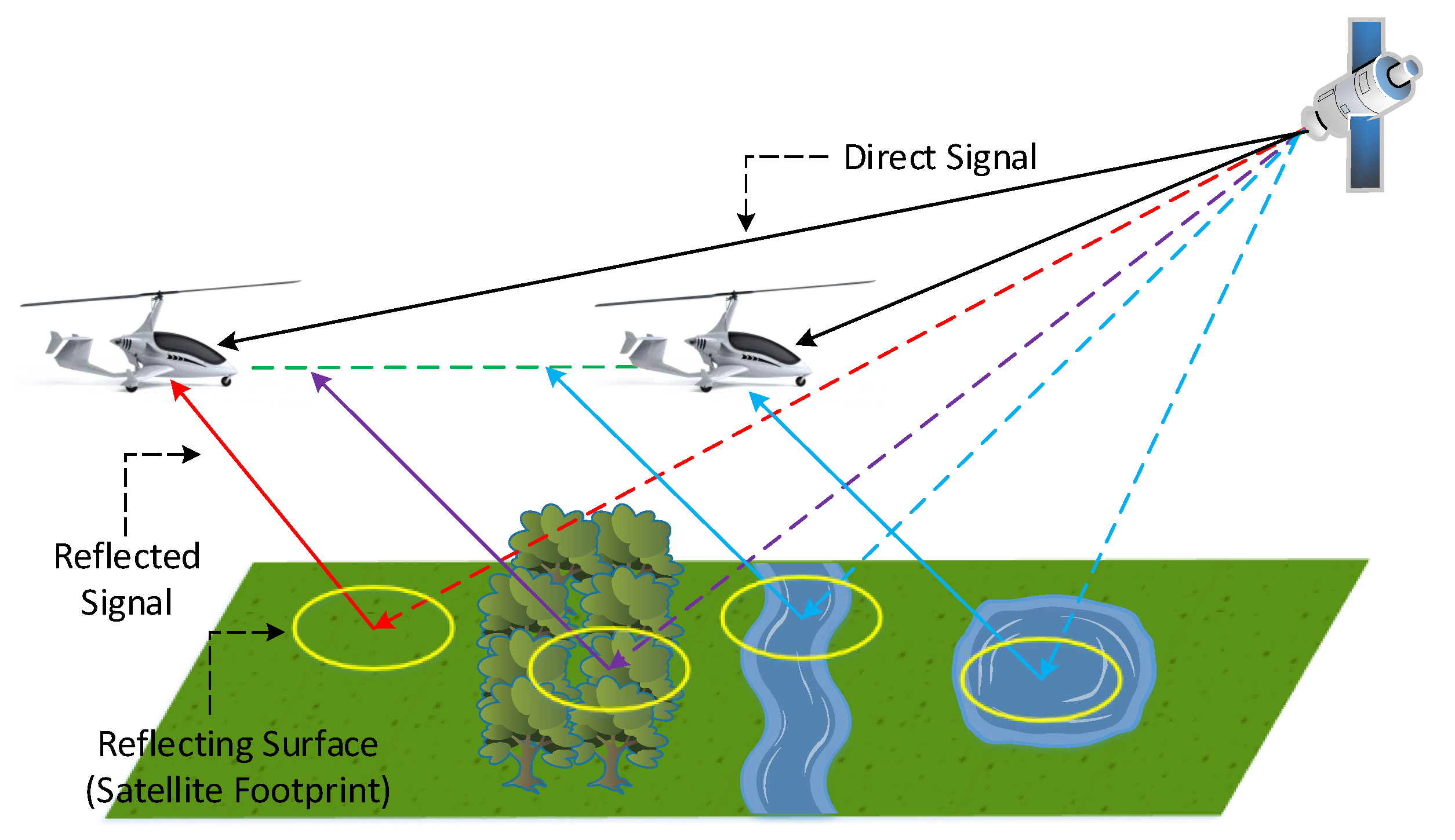
Figure 2.
Airborne GNSS-R system.
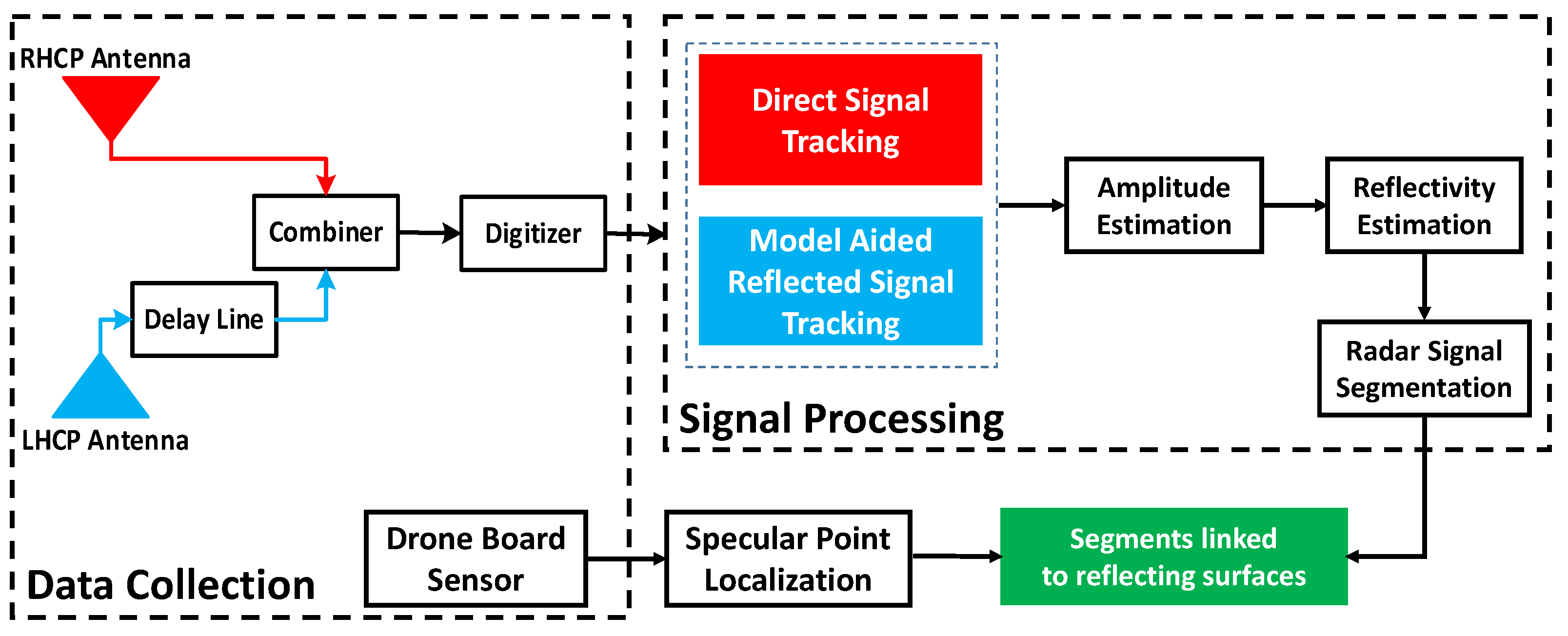
Figure 3.
Satellite footprints displacement from one area to another. The area is located at (50.888653N, 1.870741E). and represent the mean values of the GNSS signal amplitudes when the ellipses are on land and on water, respectively.
Figure 3.
Satellite footprints displacement from one area to another. The area is located at (50.888653N, 1.870741E). and represent the mean values of the GNSS signal amplitudes when the ellipses are on land and on water, respectively.
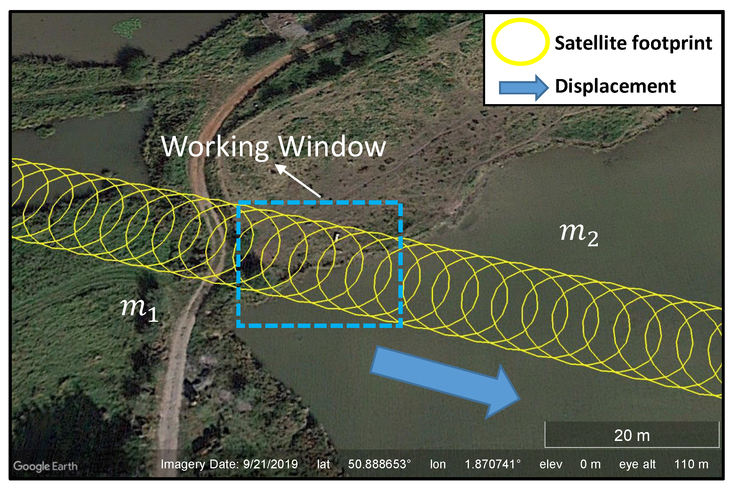
Figure 4.
Signal model in a working window. and represent the mean values of the GNSS signal amplitudes when the ellipses are on land and on water, respectively.
Figure 4.
Signal model in a working window. and represent the mean values of the GNSS signal amplitudes when the ellipses are on land and on water, respectively.

Figure 5.
Architecture of the change point detector.

Figure 6.
GNSS signal amplitude and filter innovation as a function of time.
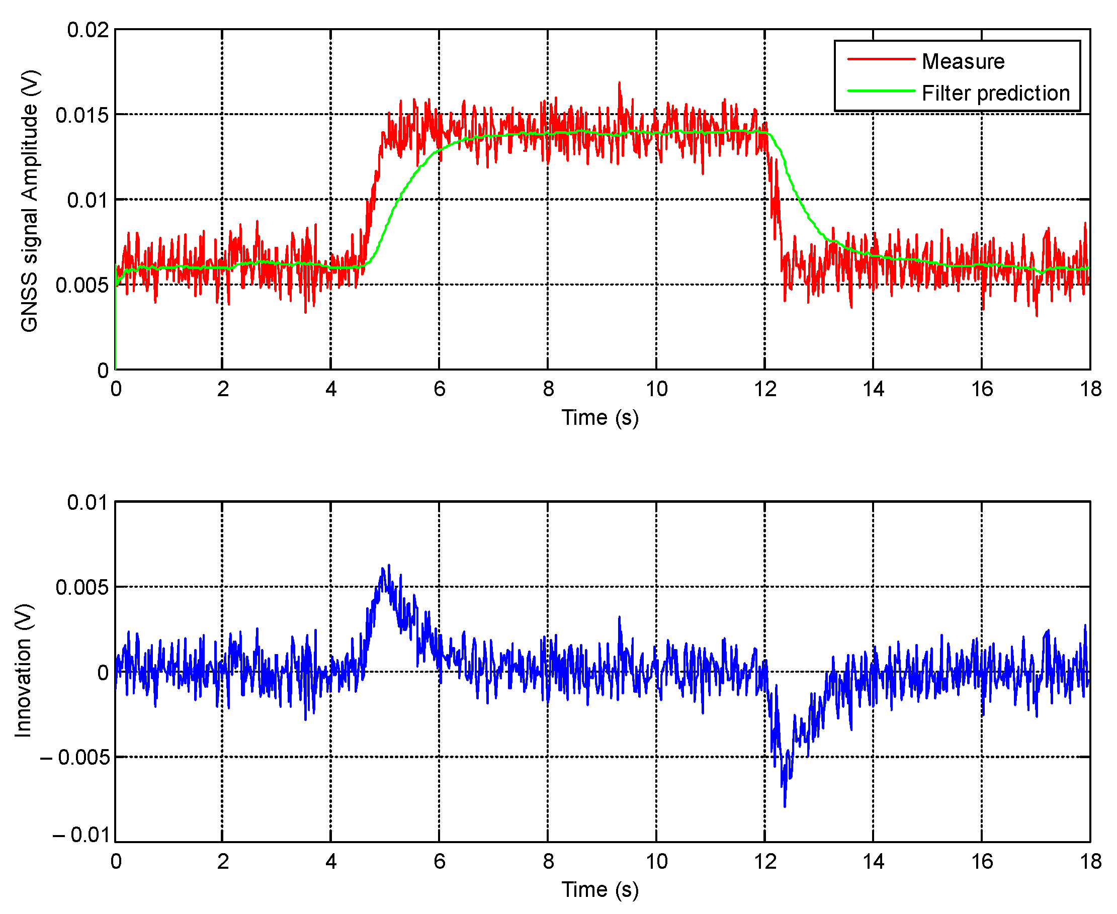
Figure 7.
Architecture of the change point localization algorithm. MLLE stands for Maximum Likelihood Localization Estimate.
Figure 7.
Architecture of the change point localization algorithm. MLLE stands for Maximum Likelihood Localization Estimate.
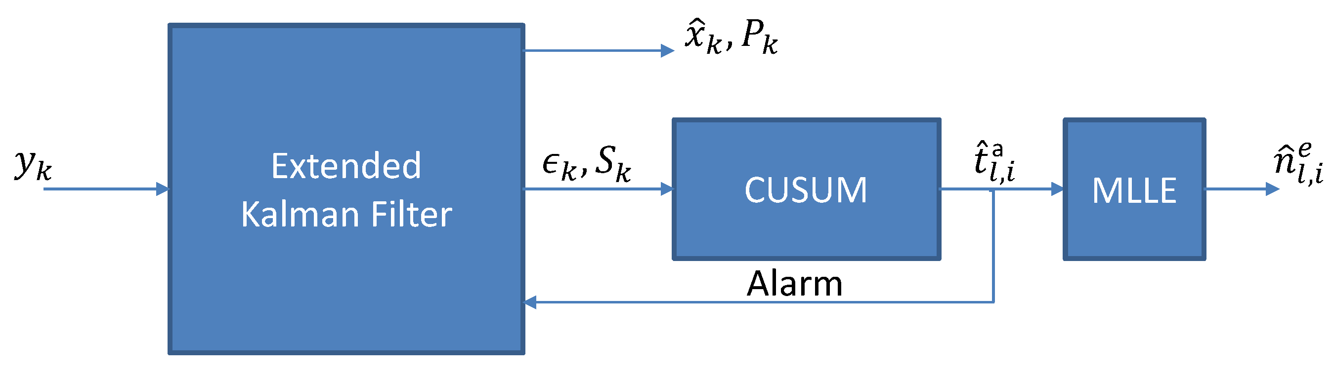
Figure 8.
Change detection and localization. (a) change detection, (b) change localization.
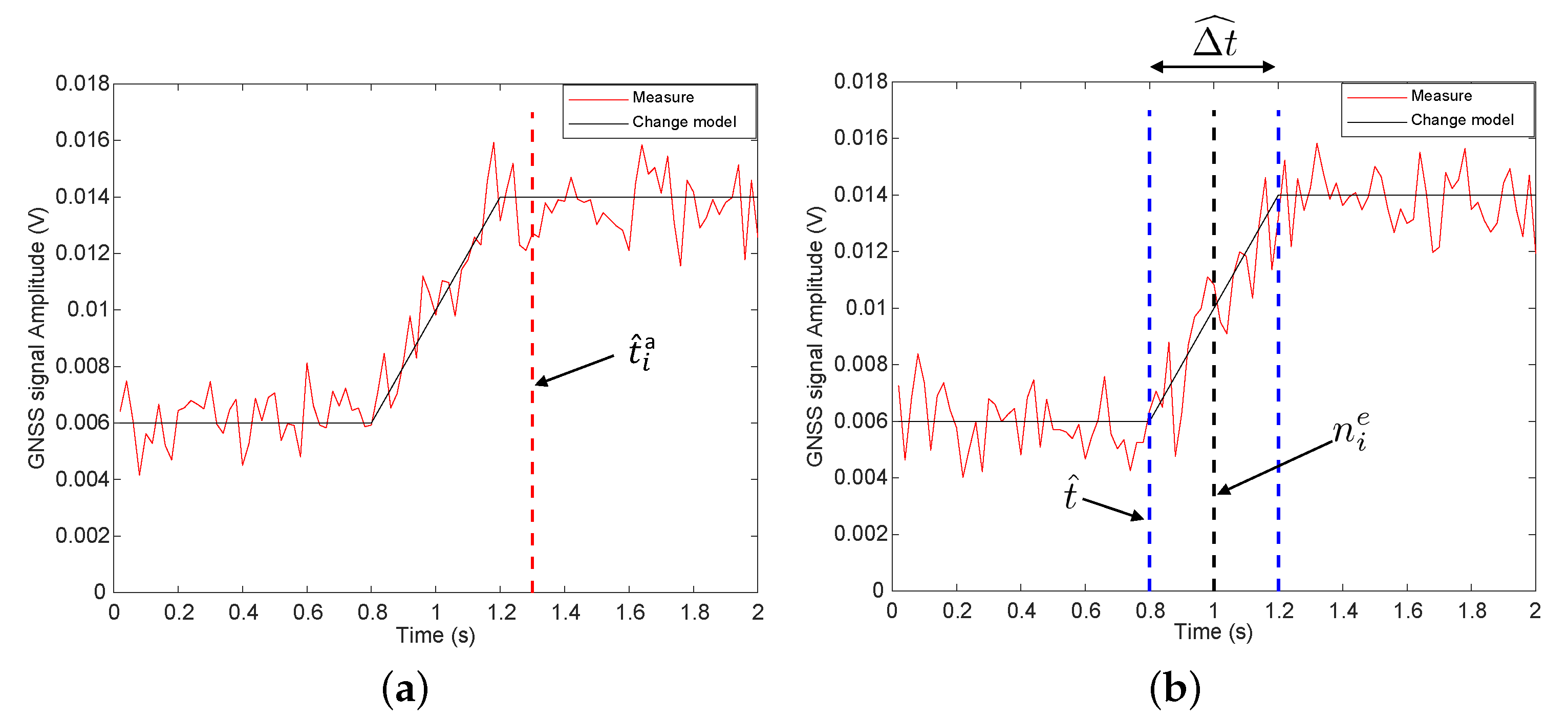
Figure 9.
Segmentation of a GNSS signal obtained in an airborne experiment. (a) detection, (b) localization, (c) segmentation.
Figure 9.
Segmentation of a GNSS signal obtained in an airborne experiment. (a) detection, (b) localization, (c) segmentation.

Figure 10.
The gyrocopter that was used during the flight with the sensors embedded on it.
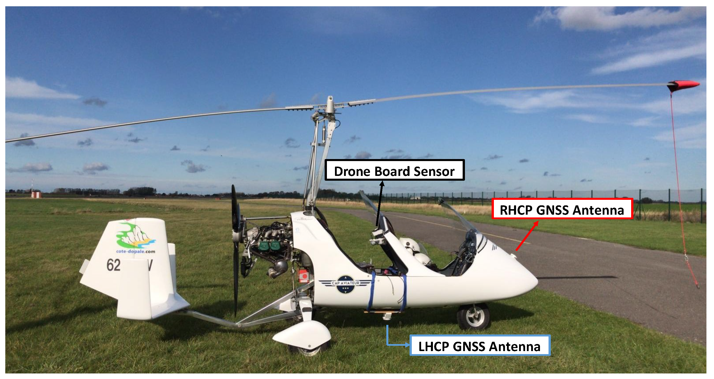
Figure 11.
Flight trajectory. Geographical setting of the study area (the WGS84 Universal Transverse Mercator UTM datum corresponds to Zone 31U North.)
Figure 11.
Flight trajectory. Geographical setting of the study area (the WGS84 Universal Transverse Mercator UTM datum corresponds to Zone 31U North.)
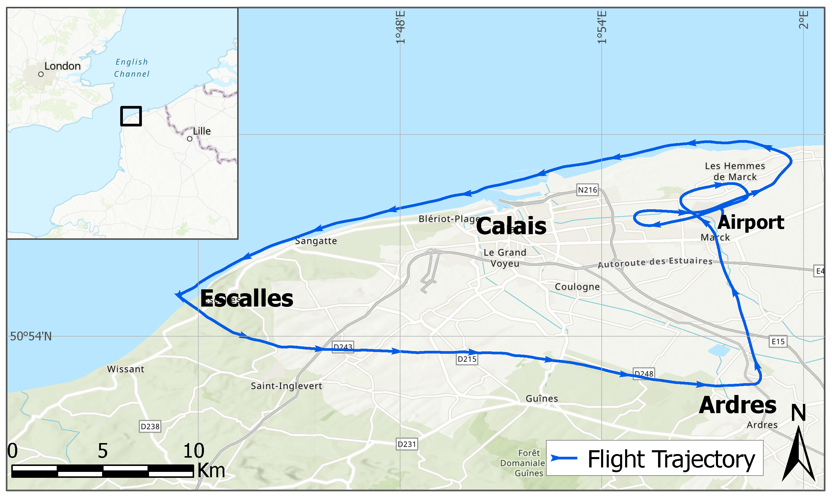
Figure 12.
The satellite footprint traces along the flight trajectory imposed on Google Earth software. The traces of very low elevation satellites are not shown in the figure.
Figure 12.
The satellite footprint traces along the flight trajectory imposed on Google Earth software. The traces of very low elevation satellites are not shown in the figure.
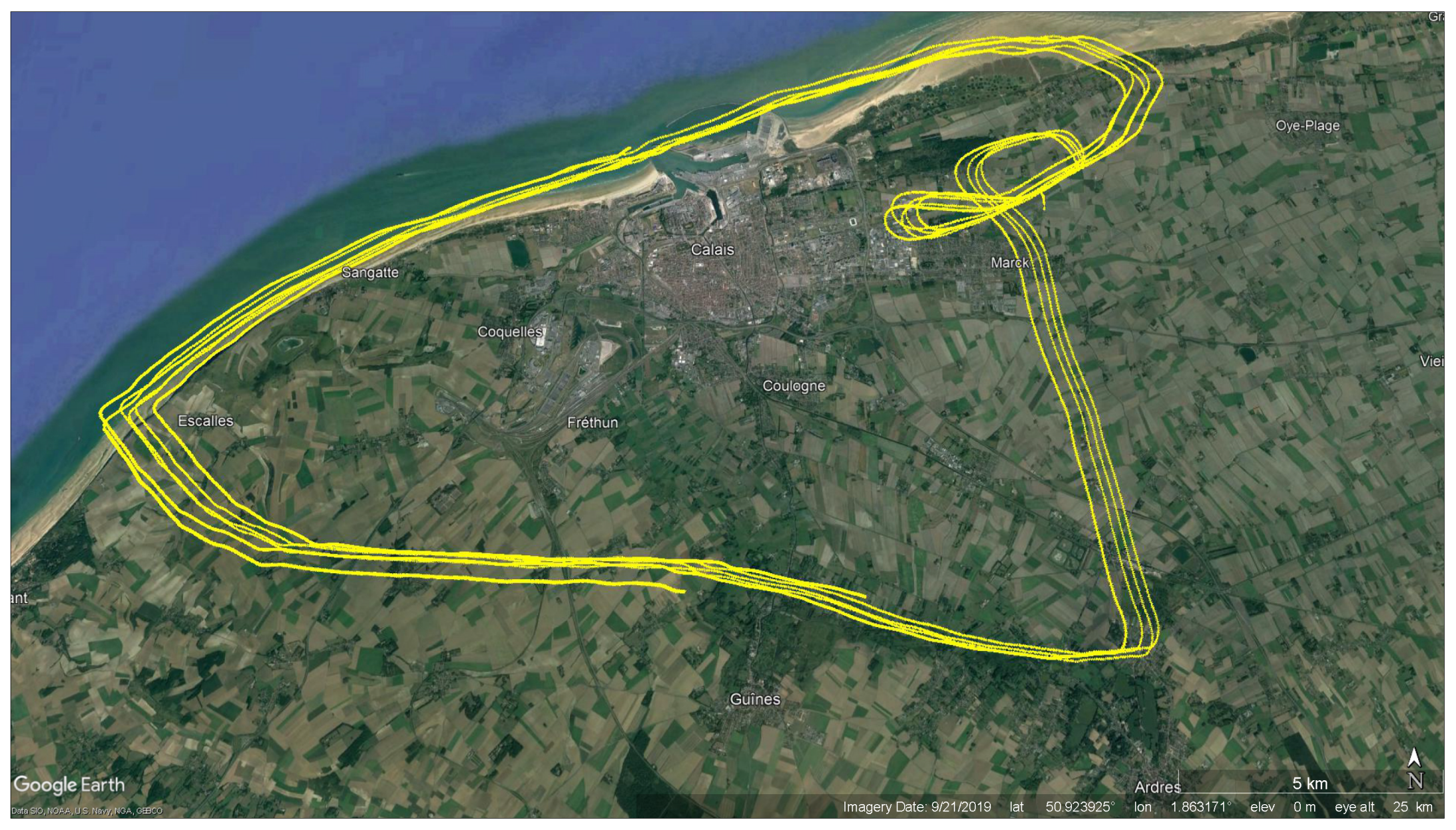
Figure 13.
Automatic segmentation of the GNSS measurements by the proposed radar technique for an area located at (50.888515°N, 1.871803°E) along the trajectory.
Figure 13.
Automatic segmentation of the GNSS measurements by the proposed radar technique for an area located at (50.888515°N, 1.871803°E) along the trajectory.
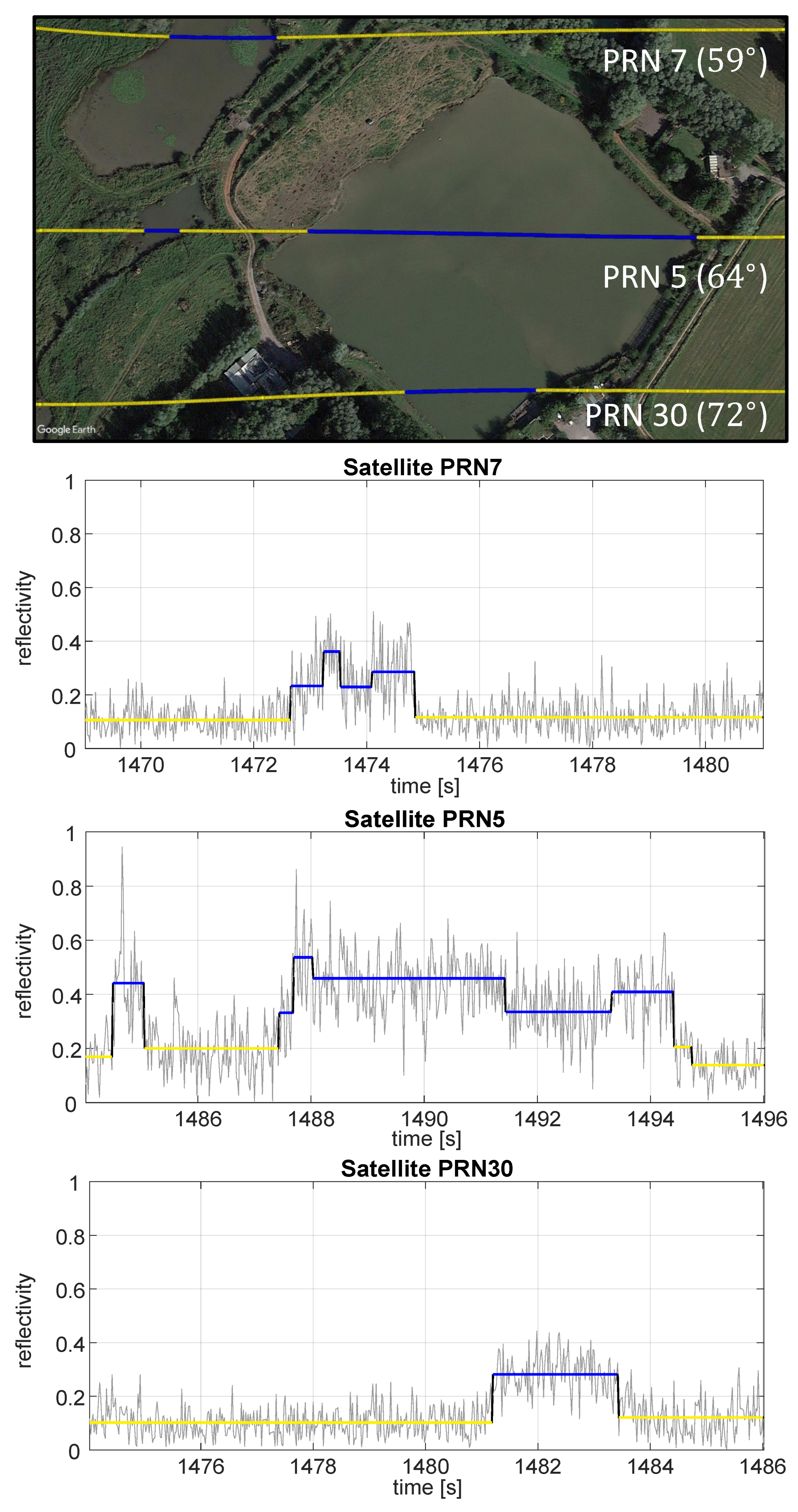
Figure 14.
Detection of water body surfaces in landforms using the proposed automatic radar technique. (a) Lake (50.882083°N, 1.976546°E); (b) Swamp (50.876854°N, 1.948390°E); (c) River (50.887720°N, 1.878526°E); (d) Streams (50.888385°N, 1.868127°E); (e) Wetland (50.883070°N, 1.900203°E); (f) Pool (50.886888°N, 1.884547°E).
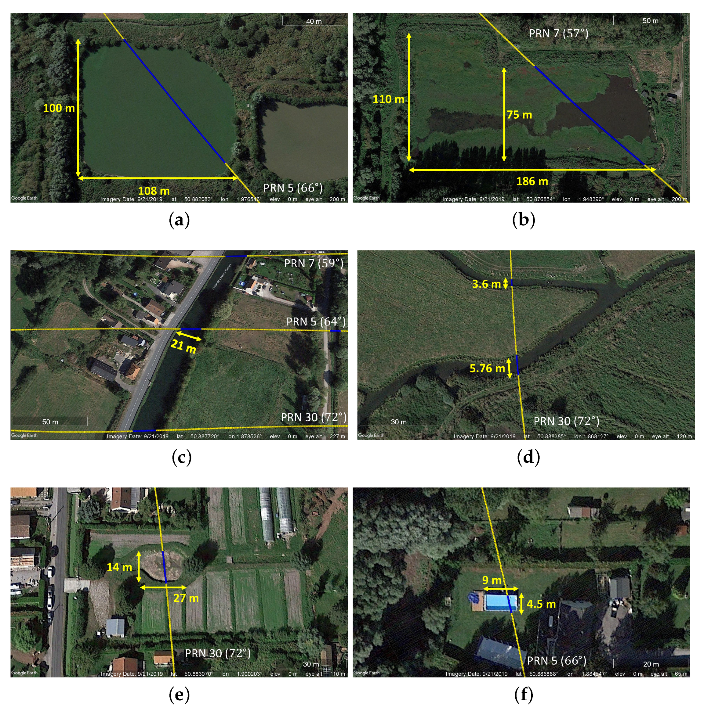
Figure 15.
The detected water body surfaces using our proposed radar technique for the area between Guînes and Ardres. The specular points of reflection, represented by a blue coloring, are superimposed on IGN maps.
Figure 15.
The detected water body surfaces using our proposed radar technique for the area between Guînes and Ardres. The specular points of reflection, represented by a blue coloring, are superimposed on IGN maps.
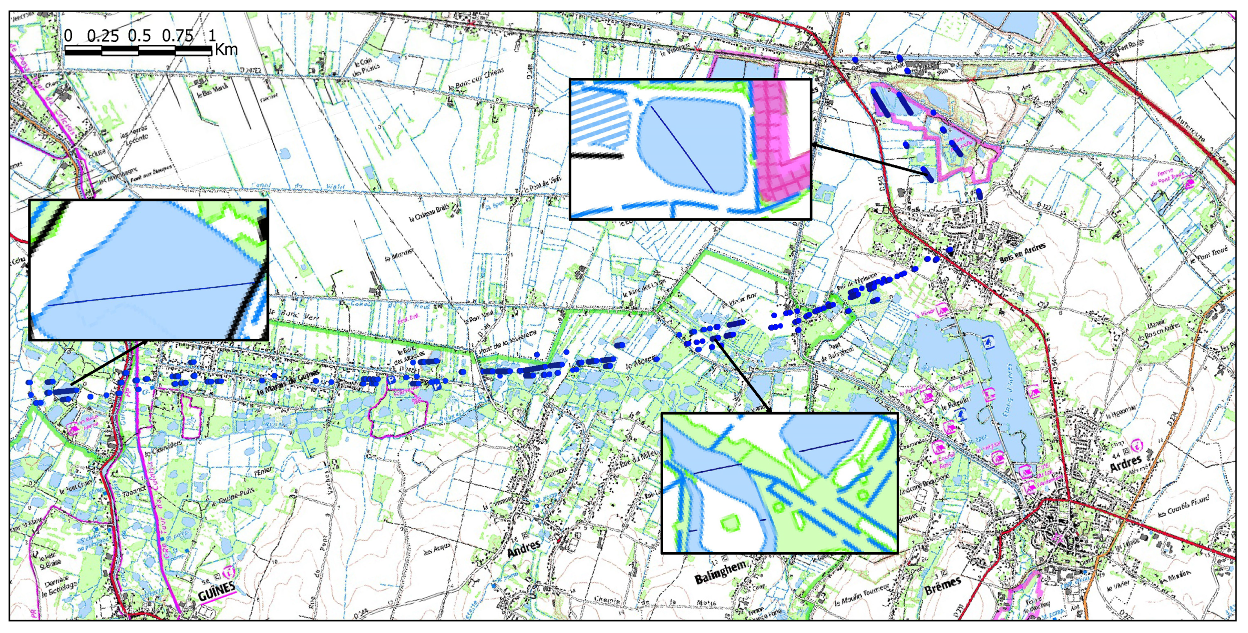
Figure 16.
Statistics of water body edge localization by the proposed radar technique per water body type.
Figure 16.
Statistics of water body edge localization by the proposed radar technique per water body type.


Table 1.
Flight Information.
| Description | |
|---|---|
| Date | 19 October 2020 |
| Location | North of France |
| Fight Duration | 45 min |
| Distance Covered | 71 km |
| Average Speed | 95 km/h |
| Average Height | 315 m |
| Wind Speed | 25 km/h |
| Wind Direction | North |
Table 2.
Performance assessment of the proposed radar technique for water body surface detection. Results of the manual inspection applied between the IGN images and our radar technique per water body type and in total (bold) for the study area.
Table 2.
Performance assessment of the proposed radar technique for water body surface detection. Results of the manual inspection applied between the IGN images and our radar technique per water body type and in total (bold) for the study area.
| Water Body | Number of Surfaces Using IGN Maps | Percentage of Detection Using Our Radar Technique |
|---|---|---|
| Lakes/Large Swamps | 20 | 100% |
| Ponds/Swamps/Wetlands | 17 | 94% |
| Rivers/Canals | 4 | 100% |
| Streams/Brooks | 6 | 83% |
| Total | 47 | 96% |
Table 3.
Parameters of the detected water body surfaces by satellite PRN 5 trace for 100 s corresponding to an area located between (50.888837°N, 1.869701°E) and (50.887512°N, 1.880296°E) along the trajectory.
Table 3.
Parameters of the detected water body surfaces by satellite PRN 5 trace for 100 s corresponding to an area located between (50.888837°N, 1.869701°E) and (50.887512°N, 1.880296°E) along the trajectory.
| Water Body | Wetland | Lake | River | Stream |
|---|---|---|---|---|
| Approximate size (m) | ||||
| Localization diff—Start (m) | 0 | |||
| Localization diff—End (m) | 0 | 0 | 0 | |
| Distance error—Total (m) | 0 | |||
| Automatic detection length (m) | ||||
| Manual detection length (m) |
Table 4.
Assessment of the accuracy of proposed radar technique for water body edge localization. Quantitative analysis of the difference between the automatic and manual edge localization for the detected water body surfaces by the traces of the 3 satellites footprints along the whole trajectory per water body type and in total (bold).
| Water Body | Number of Detections | Percentage of Perfect Edge Localization | Mean Distance Localization Error (in Meters) | Localization Difference—Std (in Meters) |
|---|---|---|---|---|
| Lakes | 12 | |||
| Oxbow Lakes | 4 | |||
| Ponds | 11 | |||
| Pools | 1 | |||
| Rivers/Canals | 12 | |||
| Streams/Brooks | 6 | |||
| Swamps | 15 | |||
| Wetlands | 4 | |||
| Total | 76.2% | 0.96 | 0.9 |
Publisher’s Note: MDPI stays neutral with regard to jurisdictional claims in published maps and institutional affiliations. |
© 2021 by the authors. Licensee MDPI, Basel, Switzerland. This article is an open access article distributed under the terms and conditions of the Creative Commons Attribution (CC BY) license (https://creativecommons.org/licenses/by/4.0/).
Share and Cite
MDPI and ACS Style
Issa, H.; Stienne, G.; Reboul, S.; Raad, M.; Faour, G. Airborne GNSS Reflectometry for Water Body Detection. Remote Sens. 2022, 14, 163. https://doi.org/10.3390/rs14010163
AMA Style
Issa H, Stienne G, Reboul S, Raad M, Faour G. Airborne GNSS Reflectometry for Water Body Detection. Remote Sensing. 2022; 14(1):163. https://doi.org/10.3390/rs14010163
Chicago/Turabian StyleIssa, Hamza, Georges Stienne, Serge Reboul, Mohamad Raad, and Ghaleb Faour. 2022. "Airborne GNSS Reflectometry for Water Body Detection" Remote Sensing 14, no. 1: 163. https://doi.org/10.3390/rs14010163
Note that from the first issue of 2016, this journal uses article numbers instead of page numbers. See further details here.