
Entropy Metrics of Radar Signatures of Sea Surface Scattering for Distinguishing Targets

Ocean Sensing Laboratory, Navigation Institute, Jimei University, Xiamen 361021, China
*
Author to whom correspondence should be addressed.
Remote Sens. 2021, 13(19), 3950; https://doi.org/10.3390/rs13193950
Submission received: 9 August 2021
/
Revised: 20 September 2021
/
Accepted: 29 September 2021
/
Published: 2 October 2021
(This article belongs to the Special Issue Advances on Radar Scattering of Terrain and Applications)
Abstract
:This paper analyzes sea clutter by a random series without assuming the scattering being independent. We quantitated the complexity of sea clutter by applying multiscale sample entropy. We found that above certain wave heights or wind speeds, and for HH or VV polarization, the target can be distinguished from sea clutter by regarding (i) the sample entropy at large scale factors or (ii) the complexity index (CI) as entropy metrics. This is because the backscattering amplitudes of range bins with the primary target were found equipped with the lowest sample entropy at large scale factors or the lowest CI compared to that of range bins with sea clutter only. To further cover low-to-moderate sea states, we constructed a polarized complexity index (PCI) based on the polarization signatures of the multiscale sample entropy of sea clutter. We demonstrated that the PCI is yet another alternative entropy metric and can achieve a superb performance on distinguishing targets within 1993’s IPIX radar data sets. In each data set, the range bins with the primary target turned to have the lowest PCI compared to that of range bins with sea clutter alone. Moreover, in our experiment using 1993’s IPIX radar data sets, the PCIs of range bins with sea clutter only were almost the same and stable in each data set, further suggesting that the proposed PCI metric can be applied in the presence of no or multiple targets through proper fitting curves.
1. Introduction
Detecting surface targets on the sea surface finds wide applications, including but not limited to navigation security (e.g., anti-collisions), law enforcement (e.g., illegal fishing), maritime surveillance, and emergency responses or rescues [1], just to name a few. Sea clutter, which refers to the radar echo amplitudes of a patch of the sea surface, is commonly recognized as one of the stumbling blocks in achieving stable and convincible radar performances on detecting surface/floating targets on the sea surface, notably those targets with a small radar cross section (RCS) and under high sea conditions. Relevant studies on this topic have been carried out in the past decades, macroscopically speaking, and the proposed methods in previous studies were all based on single or joint characteristics of sea clutter or targets, say, amplitude distributions and predictions, fractal or chaotic properties, the targets’ polarimetric characteristics, information entropy, complex entropy rate, and signal time–frequency analysis (doppler spectrum features, etc.) [2,3,4,5,6,7,8,9,10,11,12,13,14,15,16,17,18].
One of the most fundamental characteristics of radar echo amplitudes is the scattering signal statistics. Starting with five assumptions [19], the Rayleigh distribution is commonly applied to model the radar backscattering from terrain surfaces and then is modified to Rician or Weibull distributions in the presence of strong coherent scattering centers [19,20,21]. The high-resolution radar-returned amplitudes from the sea surface are well modeled by the K distribution [2,3], in which the shape parameters are estimated from measured amplitudes. Figure 1 depicts the probability density of the radar echo amplitudes of two range bins selected from the data sets (for more details, see Section 2) we applied in this study, accompanied by their estimated shape parameters, which are dependent on the range bin size, incident grazing angle, sea states, and radar parameters (e.g., operating frequency, resolutions). This can be evidently observed from Figure 1 by comparing the probability densities from pure sea clutter and the primary target. Although the radar performances were significantly enhanced by applying adaptive techniques to guarantee a constant false alarm rate (CFAR), the statistical models are still not effective [11]. Besides, the probability density function (PDF) itself is not enough in characterizing a random series; one vivid case is that a Gaussian-distributed white noise series can be transformed into a Gaussian-distributed pink noise series through rearranging the elements’ orders only, while the latter has a totally different power spectral density (PSD) function and turns out to be fractal [22].
We have noticed that ocean waves are fractal in nature, and sea clutter is deduced and observed to be fractal. The fractal structures and metrics have been widely applied to model sea clutter or detect targets [4,5,6,7,8]. To characterize the fractal properties of radar echo amplitudes, e.g., in [11], sea clutter is assumed as a random walk process in time, and whether the scaling law [11]
hold is further examined. In Equation (1), m, n, and q are all positive integers, and the average processes on the left-hand side should be conducted under all possible pairs to generate the series. With proper fitting curves and by setting , the Hurst parameter is estimated for backscattering amplitudes of each range bin. Sea clutter strongly exhibits multifractal behaviors and is non-stationary in the timescale range of about from 0.01 s to a few seconds. It has been observed that a significant difference in the estimated Hurst parameter exists between the range bins with and without a target under sea clutter, implying that the Hurst parameter can be an alternative metric for detecting surface targets (HH polarization only). For this reason, the authors of [11] claimed that the scattering statistics only offer a limited physical understanding of sea clutter and are not effective in detecting targets under sea clutter.
We also noticed that the condition of using the Hurst parameter as a metric is that sea clutter must be treated as a random walk process but not non-stationary. Thus, both the scattering statistics and the Hurst parameter metric are based on an independent scattering assumption. More specifically, in scattering statistics, interactions among N scatters within the antenna-illuminated area are ignored; the total scattered field is then simply a linear superposition of the scattered field of each scatter,, as shown in Figure 2, that is,
where is the amplitude and is the associated random phase. Under the random walk process, the scattered fields in each range bin are assumed independent of each other at different sampling. That is, the temporal correlation is not yet considered.
The above discussions lead us to attempt two objectives: (i) treating the backscattering amplitudes as a random series without physical assumptions and (ii) exploring a metric that can distinguish the surface/floating targets in sea clutter. From previous studies [23,24,25,26,27], we found that the multiscale sample entropy (MSE) might be a good candidate due to the following facts:
- (i)
- (ii)
- The entropy kernel applied in the MSE algorithm was investigated for complex dynamics such as non-stationary or long-range correlations in [24], and it affords theoretical evidence for applying the MSE to radar signals, particularly to sea clutter, which turns out to have fractal or non-stationary characteristics [11].
- (iii)
- Compared to the information or complex entropy metrics [15,17], the MSE algorithm guarantees showing both statistical and fractal properties, qualitatively. It is found that under the Gaussian distribution, and the same mean and standard deviation value, the series with the exponential power spectrum density (PSD) function turns out to have larger estimating sample entropy values than that of the one with a Gaussian PSD function at each scale factor. For showing fractalities, as shown in [25,26,27], pink noise turns out to have an invariant estimated sample entropy value at all scale factors, whereas the estimated sample entropy of white noise decreases along with the increasing scale factors and becomes smaller than pink noise at large scale factors. Due to the well-known fractal properties of pink noise [22] (also explained in [25,26]), it is then reasonable to deduce that the random series is fractal if its estimated sample entropy value is invariant within a certain range of scale factors.
- (iv)
Following this, we attempt to explore the feasibility of using the MSE or its variants as metrics in detecting a surface target in sea clutter. The rest of this paper shows our endeavors in detail and is organized as follows: Section 2 first introduces the data sets we selected as test samples, Section 3 presents the details and discussions of the MSE algorithm and how the proposed entropy metrics were constructed step by step, Section 4 validates and discusses the performances of the proposed entropy metrics, and finally, a conclusion is drawn to close this paper.
2. Data Description
The sea clutter data applied in this study were obtained from the IPIX radar website [28]. The McMaster IPIX radar operates at X band with a frequency of 9.39 GHz and dual polarization (H and V). The 1993’s data sets contain 14 sets; each data set includes 14 range bins, and we then have a total of 392 (14 × 14 × 2) data series. Each range bin contains 131,072 (217) numbers, and with a sample interval of 1 ms, the data of each range bin last for about 2 min (131.072 s). The target was made of a spherical block of Styrofoam with a diameter of 1 m and was wrapped with a wire mesh. As an example, Figure 3 depicts the backscattering amplitudes of some range bins in data set 54 and intuitively shows the differences between HH and VV polarizations, sea clutter only, and the target.
Due to the oversampling in range dimension, the target then hits a few range bins. The range bins, except with the primary target, are therefore remarked as containing a secondary target. Table 1 presents more details of these 14 data sets, accompanied by wave heights, wind speeds, and their corresponding sea states. Unlike the data descriptions in [11], where the wind speeds or wave heights were generally summarized for all of 1993’s data sets, we searched and outlined the sea conditions for each data set separately. From the website, we noticed that the wind speeds for the data sets can only be recorded as higher or lower than 5.56 m/s; however, the data set 54 data with wind speed being around 20 km/h (about 5.56 m/s, or 11 knots) can be clearly identified. Their corresponding sea states were estimated according to the wave height, and the Douglas scale was applied instead of the standard proposed by the World Meteorology Organization (WMO) [3].
Note that in Table 1, if the instantaneous wind speeds were set as the metric in estimating the sea state, then the sea states given in Table 1 were over- or underestimated, given rise by the complicated nonlinear air–wave interactions and many other factors, such as wind fetch and wave age. In Table 1, data sets 310, 311, and 320 were all with low sea states but at higher wind speeds. Hereafter, we treated the cases with both low sea states and wind speeds as low or moderate sea conditions. For simplicity, we classified the cases with high sea states or wind speeds as high sea conditions. Thus, these 14 data sets covered typical sea conditions.
3. Methodologies, Feasibility Analysis, and Entropy Metrics Construction
This section gives the basics of the MSE algorithm and three additional remarks. After that, the MSE under a general template vector length of 14 data sets is calculated for HH and VV polarizations. Based on the calculated MSE, two entropy metrics, namely sample entropy (SampEn) at large scale factors and the CI, described under high sea conditions only. To consider the low or moderate sea conditions, we make use of the polarization signatures of the calculated MSE, a nonlinear polarization combination, and the PCI metric.
3.1. Brief Reviews on the MSE Algorithm
The MSE algorithm [25,26] contains two main procedures: coarse graining and SampEn estimations. For a data series with length , the coarse graining is mathematically given by
where ; denotes the identity number of elements in the original series and the coarse-grained subseries ; and is the scale factor that determines the length of coarse-grained subseries. It is readily seen from Equation (3) that the original series corresponds to the scale factor at , that is, .
For each coarse-grained series (including the original one), the SampEn estimation [25,29] is applied. The SampEn of a series is defined as
where denotes the ID of the elements in series ; is a preset template vector length and determines the dimension of the template vector; and is a threshold: a commonly selected value is , where std denotes the standard deviation, and constants 0.15 or 0.2 are the default ones in [26,27]. In addition, in Equation (4), is the number of matches of length with the k-th template and is the number of matches of length with the k-th template. More specifically, in the SampEn algorithm, the k-th template is given by
and the distance between the k-th and the l-th template vector is defined as , and means that the self-matches are precluded. Figure 4 shows a case of the k-th template vector and at . In the SampEn algorithm, the Euclidian distance between two template vectors is selected. Then, satisfies
and satisfies
It follows that for the k-th element, we have . For all k and template vectors, there exists the relationship
3.2. Remarks on the MSE and Properties
We now provide details of three additional remarks regarding the MSE.
3.2.1. Complexity Index
The complexity index, also named the area under the curve (AUC), is defined as the integrated complexity of a random series. Based on its definition, the CI is then expressed in terms of the estimated SampEn at each scale factor as
where represents the estimated SampEn under scale factor .
3.2.2. Convergence of MSE and SampEn
As shown in Section 3.1, under a certain scale factor , the estimated SampEn is determined jointly by and . If the constant in increases, then the estimated SampEn approaches zero due to an infinitely large threshold. However, if the constant is infinitely small, the estimated SampEn tends to be infinitely large. Thus, talking about the convergence of SampEn under the parameter is meaningless, and like mentioned before, 0.15 or 0.2 is the default constant in . Now, only the effects on estimating SampEn of template vector length remain to be investigated. It can roughly be deduced from Equations (6) and (7) that the Euclidian distance between two template vectors increases along with increasing . Then, for a fixed , there must be a maximum template vector length , and for template vectors longer than the maximum one, we always have Equations (6) and (7) established simultaneously. As a result, the left-hand side of Equation (8) evolves into a constant, and so do the estimated SampEn values. The maximum template vector length is of paramount importance since the PCI metric proposed later only works under the maximum template vector length. We therefore defined and set a criterion to determine the maximum template vector length as follows.
To further exhibit the convergence of the MSE with , as an example, the SampEn of range bin 1 (sea clutter only) of data set 17 was estimated under the parameters , , and is depicted in Figure 5 for both polarizations. It is observed from Figure 5, for both polarizations and at a certain scale factor, the estimated SampEn decreases and then saturates along with increasing template vector length. To obtain , one can apply the Euclidian distance between the two MSE series, which is estimated under an adjacent template vector length and , and then compare it with a preset precision , namely
The preset precision is associated with the scale factor since the scale factor determines the length of the MSE series. Then, Equation (10) can also be regarded as comparing the mean Euclidian distance between two MSE series with . In practice, must be gauged by a given precision and a certain scale factor , instead of assigning it with the highest priority. If it is assigned first, then under large scale factors, the maximum template vector length might be underestimated due to the large values. It should be noted that each range bin in a data set has a maximum template vector length, and of a data set is defined as
where is the range bin numbers in a data set. By setting precision and under the selected scale factor in this study, then turns out to be 0.01 and is found to be 6 in this case. It is observed from Figure 5 that the obtained maximum template vector length acquires desired accuracies under these given parameters. The MSE under the maximum template vector length is also named the converged MSE.
3.2.3. Significance of the Difference
We may make use of the significance of the difference between two MSE series because (i) it can be regarded as a signature in pattern classifications and (ii) two MSE series might have overlapped error bars. Compared to the original series, the MSE series have shorter lengths, making the non-parametric test, say, the rank-sum test, more suitable. One example is that without loss of generality, if the p-value is smaller than 0.05, then the two MSE series in the rank-sum test have a significant difference and can be classified as two different patterns.
Thus, if the MSE series between sea clutter and the target have significant differences, then we could say that we can distinguish the range bins with targets from those in sea clutter. Unfortunately, after a thorough check within all range bins in 1993’s data sets, we found that the MSE series between range bins with sea clutter only are also significantly different. Thus, it is impossible to distinguish the target from sea clutter by checking the significance of the difference between the MSE series of range bins. We may conclude at this point that sea clutter cannot be simply characterized by a distribution or by specific shape parameters.
3.3. The MSE of Sea Clutter and Discussions
Following the MSE algorithm, we calculated the MSE of sea clutter for all samples under the parameters , , and template vector length [19,20]. Figure 6 and Figure 7, respectively, depict the MSE of each data set for HH and VV polarizations, presenting in the form of the imageries of matrices and .
It is observed from Figure 6 that at wave heights larger than 2.0 m (data sets 17 and 18) or at wind speeds equal to or higher than 5.56 m/s (data sets 56, 310, 311, and 320), the MSE of range bins with the primary target can be easily distinguished from that of range bins in sea clutter by (i) the estimated SampEn at large scale factors, for instance, at scale factor , and (ii) the CI introduced in Section 3.2.1 since the MSE of range bins with the primary target is smaller than that of range bins in sea clutter. Meanwhile, within the same data sets, the same performances can be observed from Figure 7 for VV polarization. From Figure 8 and Figure 9, we see that the CIs are effective under high sea conditions.
With these two metrics, we then turned to data sets with low or moderate sea conditions (data sets 19, 25, 26, 30, 31, 40, 280, and 283). It is seen from Figure 6 and Figure 7, within data sets 19, 25, 26, 30, 31, and 40, and for both polarizations, these two metrics are no longer effective, perhaps because the MSE of the range bins with the target cannot be distinguished from that of the range bins in sea clutter. data set 283 showed that for both polarizations, these two metrics are still effective, while as depicted in Figure 8h and Figure 9h, data set 280 showed the differences between polarizations, since the range bin with the target could only be distinguished by VV polarization.
Until now, it may be reasonable to conclude that for both VV and HH polarizations, these two metrics are effective, and even more so if linearly combining two polarizations. Under low or moderate sea conditions, these two metrics perform poorly. Compared to HH polarization, VV polarization performs better under all sea conditions under consideration. This is somehow different from our belief that the targets can be easy detected under a calm sea. Possible causes are deduced as follows. First, these two metrics are all entropy based to describe the complexity of sea clutter, which, under high sea conditions, is only much higher than that with the targets. The complexity of sea clutter reduces under low or moderate sea conditions, making these two metrics less pronounced and indiscernible in the presence of the targets. On the aspects of scattering mechanisms [3], under high sea conditions, the long bursts (also named whitecap modulations) and short bursts endow HH polarization with interrupted peaks (also see Figure 3). These irregular peaks then enhance the HH polarized complexity and yield a larger MSE than that of the targets. These bursts vanish under low or moderate sea conditions, and the MSE decreases.
Compared to HH polarization, VV polarization is more pronounced with Bragg modulations. For X-band radars, Bragg scattering mainly originates from the capillary gravity or capillary waves with resonance wavelengths on the sea surface, and then the wind speed has paramount importance. The interferences between these resonant waves and many other scattering components endow the VV-polarized sea clutter with larger complexity than that of the targets.
Thus, under high sea conditions, these two metrics are effective with both HH and VV polarizations. Moreover, as shown in Figure 6, Figure 7, Figure 8 and Figure 9, the VV-polarized amplitudes turn out to have higher complexity compared to the HH-polarized ones, notably under high wind speeds, suggesting that VV polarization is more sensitive to the backscattering from seawater. However, due to the complicated sea conditions and with limited test data samples, it is not yet possible to obtain a certain sea state as the standard to quantify the scope of application of these two metrics. Nevertheless, these two metrics are alternatives to existing methods in the context of target detection in sea clutter, particularly under high sea conditions.
Next, we turned to further develop an entropy metric by combining the polarization signatures of the MSE; compared to the above-mentioned two metrics, it covered all the sea conditions involved in this study.
3.4. A Non-Linear Polarization Combination for Generalities
We turned to construct another entropy metric by combining the polarization signatures of the MSE, as shown in Figure 6 and Figure 7, and ensured it is effective under all sea conditions. Obviously, for low or moderate sea conditions, where the VV- or HH-polarized MSE becomes invalid, we deduced that linear combinations of the VV- and HH-polarized MSE remain invalid. Besides, the linear relationships yielded nonunique coefficients. Then, building a nonlinear polarization combination deserved a deeper look.
From our previous tests, we saw that the MSE of VV polarization was much larger than that of HH polarization. The increasing of the MSE, from HH polarization to VV polarization, with and without sea clutter is different. We took the data sets in which the CI metric turned out to be invalid, for example, since we needed to take a deeper look into these cases. The MSE ratio, namely of data sets 25, 26, 30, 31,40, 280, and 19 were calculated under the same parameters as Figure 6 and Figure 7, and are presented in Table 2. It is seen from Table 2 that the MSE ratios of range bins with the primary target were all higher than those of the ones with sea clutter only, except data set 19, in which the range bin with the primary target had the lowest MSE ratio. When the polarized MSEs were combined, the highest or lowest MSE ratio in Table 2 corresponded to a high or low MSE compensation to the CI of the range bin with the primary target or, equivalently, a low or high compensation to the CI of range bins with sea clutter only. These compensations may yield undistinguishable CI metrics and are the risk of detecting targets by a deterministic characteristic. In other words, Table 2 suggests that we keep an eye on full use of the items (data sets 25, 26, 30, 31, 40, and 280) and (data set 19) simultaneously.
Together with these polarization signatures of the MSE, we sought a nonlinear relationship that (i) keeps the dominance of the HH- or VV-polarized MSE under high sea conditions to ensure that the target is detectable as the two former metrics did under high sea conditions, and (ii) compensates the MSE of range bins with pure sea clutter more but the MSE of range bins with targets less, to ensure that the targets are distinguishable by their lowest complexity under low or moderate sea conditions.
To this end, we started with the sigmoid function
where is a constant that controls the convergent rate of to limit. It follows that the nonlinear polarization combination is then given by
with
and
where denotes the element in the matrix and , respectively. stands for the range bin numbers, as defined in former sections. In matrix form, we have the polarization combination
or equivalently
where are all matrices. The two limits can be readily obtained from Equation (15). For VV dominance, we have , and then ; and for HH dominance, we have , and then . Thus, either the VV or the HH dominance is preserved. This corresponds to the superb performance of the VV- or HH-polarized MSE under high sea conditions. Under low or moderate sea conditions, the polarized MSE of sea clutter and targets determines the ratios and the abscissa’s location in the sigmoid function. Finally, following the CI in Equation (9), the polarized complexity index (PCI) is defined as
The is a vector with length and is regarded as a novel entropy metric. The PCI performance was validated under different template vector lengths in the next section.
4. Performance
This section validates the PCI performances under different template vector lengths, and other parameters in the MSE are set at and . Section 3.2.2 explains why the threshold and scale factor can be fixed at certain values.
4.1. Performance under the General Template Vector Length
Under the general template vector length , the PCI defined in Equation (18) of all 14 data sets was calculated and is depicted in Figure 10. We see from Figure 10 that the PCI significantly improved the detection performance under low or moderate sea conditions; that is, the primary targets in data sets 25, 26, 30, 31, and 40 now could be distinguished in sea clutter for their lowest PCIs. However, the target in data set 19 was still unable to be detected, and the PCI under the general-template vector length even showed poorer performance in data set 17. Clearly, a better solution is desirable. In line with this, we cameup with the template vector length gauged by the converged MSE.
4.2. Performance under
Following Section 3.2.2, the maximum template vector length of the 14 data sets was obtained as . Similar to Figure 10, the PCIs of all 14 data sets were then calculated and are shown in Figure 11.
From Figure 11, we see that the range bins with the primary target now all had the lowest PCIs compared to other range bins without a target. In data set 17, the range bins 10 and 11 with the secondary target has lower PCIs than range bin 9 with the primary target, and the PCI of the range bin in data set 17 with the primary target was smaller than that of any range bins without targets. Thus, we may conclude that the PCI performed well for all 14 data sets. Furthermore, precluding the range bins with secondary targets, the range bin with the primary target showed the lowest PCI value compared to the range bins with sea clutter and could be distinguished from those range bins without targets. Then, the lowest PCI of range bin 9 in data set 17 showed the law we found in other data sets. It is also worth noting that even for , the SampEn at large scale factors and the CI were not effective under low or moderate sea conditions.
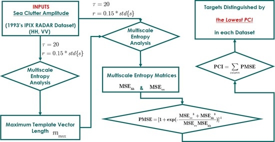
In what follows, we summarize the procedures of applying the PCI metric in terms of a pseudo-algorithm.
4.3. Procedures of Applying the PCI Metric
For simplicity, details of the classical MSE algorithm are omitted here and can be found in [25,26]. Applying the PCI metric consists of three main steps:
- Under the defaulted scale factor and threshold, obtaining the maximum template vector length
- Under , the defaulted scale factor and threshold, constructing the MSE matrix and for both polarizations
- Constructing the matrix by Equations (16) or (17) and calculating the PCI for each range bin by Equation (18), followed by finding the smallest PCI value and recording its corresponding range bin identity number, which is then recognized as containing the target.
The pseudo-algorithm of the procedures outlined above is presented in MATLAB® customs in Appendix A.
5. Discussion
Unlike the scattering statistics or the Hurst parameter in the fractal model, the basis of the three proposed entropy metrics in this study emphasizes the complexity differences between with and without targets in sea clutter. As shown in Figure 6, Figure 7, Figure 8 and Figure 9, for HH or VV polarization, SampEn at large scale factors and the CI are only effective under high sea conditions. However, the proposed PCI metric is effective as a target detector in sea clutter under all sea conditions. More specifically, the range bins with targets were all found to have the lowest PCI within 1993’s IPIX radar data sets.
For practical use of the PCI, we have to preset a threshold such that a minimum PCI difference between with and without targets is detectable. In Figure 11, the minimum PCI difference occurred in data set 310, and the PCI difference between range bins 1 and 7 was 0.1289. For all the 14 data sets, if the PCI difference between the range bin with the lowest PCI and any one of the remaining range bins was smaller than 0.1289, then the range bin with the lowest PCI was recognized as sea clutter only (the fake target). Conversely, it would be recognized as the real target.
One question is how to deal with cases with no or multiple targets. Indeed, to achieve the desired CFARs, it is necessary to set a threshold adaptively. A unique property of the proposed PCI metric in the context of surface target detection in sea clutter found in this study is helpful. We can see from Figure 11 that the PCIs of range bins with sea clutter only were relatively stable in all data sets. The sudden bursts, e.g., range bin 2 in data set 18, range bin 4 in data set 25, and range bin 10 in data set 26, can be smoothed or even eliminated by applying proper filtering. The result is that for one or multiple targets, only one or few obvious inflection points (with the lowest PCI) are left. For sea clutter only (no target), the PCI curve flattens without presenting dominant inflection points.
6. Conclusions
We quantitatively investigated the complexities of sea clutter using multiscale entropy measures without assuming the scattering being independent. From extensive tests on the 1993’s IPIX radar data sets under high sea conditions, we found that the entropy metric is able to effectively discern the surface targets in sea clutter. An entropy metric, PCI, that combines the polarization signatures was proposed to render itself as an effective target detector under low-to-high sea conditions.
The proposed entropy metrics show potential in applications of marine radar target detection as an alternative to current known methods. The following observations are in order:
First, the coarse graining in Equation (3) is equivalent to the incoherent accumulations in radar signal processing. Consequently, the temporal correlation effects were ignored in SampEn under large scale factors.
Second, the averaging in coarse graining essentially is a lowpass filter such that the long or short bursts in HH polarization can be filtered out. It helps explain why SampEn slowly saturates at HH polarization than at VV polarization.
Finally, the fractal properties of sea clutter are fully contained and exhibited by the MSE. The invariant SampEn with the scale factor of pink noise confirms that sea clutter is fractal. Results indicate that both HH-polarized and VV-polarized sea clutter shows fractal properties at larger and smaller scale factors under high sea conditions, respectively. The difference in fractal properties also implies that the VV-polarized scattering is more sensitive to Bragg resonance and is less impacted by whitecaps or breaking waves.
Author Contributions
Conceptualization, R.J. and L.-N.L.; methodology, R.J.; software, R.J.; formal analysis, R.J.; investigation, Q.S., S.-Z.H., J.-J.G., and X.-H.X.; writing—original draft preparation, R.J.; writing—review and editing, R.J. and L.-N.L.; supervision, R.J.; project administration, R.J., L.-N.L., Q.S., S.-Z.H., J.-J.G., and X.-H.X.; funding acquisition, R.J., L.-N.L., Q.S., S.-Z.H., J.-J.G., and X.-H.X. All authors have read and agreed to the published version of the manuscript.
Funding
This research was funded by the Project of Intelligent Situation Awareness System for Smart Ship (grant no. MC-201920-X01), the National Natural Science Foundation of China (grant no. 42001318), the Start Research Funding from Jimei University (grant nos. ZQ2021022 and HHXY2020018), and the International Joint Laboratory of Polarimetric Sensing and Intelligent Signal Processing, Xuchang University.
Acknowledgments
The authors are grateful to Simon Haykin of the McMaster University of Canada for sharing the IPIX radar data sets with common users, and the anonymous reviewers for help improving the quality of this paper. We especially thank Frank Lin, the CEO of Tianwu Ocean Tech. Co., for his support of this study.
Conflicts of Interest
The authors declare no conflict of interest.
Appendix A
The appendix is presented for showing the main procedures of realizing the proposed PCI metric, without loss of generalities, and the pseudo-algorithm is given in MATLAB language format.
| Step 1: Obtain the Maximum Template Vector Length-Mmax |
| Input: Scale Factor: tao = 20; Amplitude Series: Si, i = 1, 2, 3, …, rb; Threshold: tao*c = 0.2 |
| for i = 1:rb |
| ri = 0.15*std{Si}; %Threshold in MSE algorithm |
| for m = 1 |
| MSE(i,m) = MSEA(tao, ri, m, Si); % MSEA: MSE algorithm |
| MSE(i,m + 1) = MSEA(tao, ri, m + 1, Si); |
| dMSE(i) = Euclid {MSE(i,m + 1),MSE(i,m)}; % Euclid: Euclidian distance |
| if(dMSE(i) < tao*c) |
| Mi = m+1; |
| else |
| m = m+1; |
| end for |
| end for |
| Mmax = max {M1, M2, M3, …, Mrb}; |
| Step 2: Construct the MSE Matrices–MSE (pol) |
| Input: Pol: HH or VV; Amplitude Series: Si, i = 1, 2, 3, …, rb; Scale Factor: tao = 20; Mmax |
| for i = 1:rb |
| ri = 0.15*std{Si}; |
| MSE(i, pol) = MSEA(tao, ri, Mmax, Si); |
| end for |
| MSE(pol) = MSE; % Dimension: tao*rb |
| Step 3: Calculate the PCI |
| PMSE = PMSEA(MSE(HH), MSE(VV)); % PMSEA: Equation (16) or (17) |
| PCI = column-sum(PMSE); |
References
- Bole, A.; Wall, A.; Norris, A. Radar and ARPA Manual: Radar, AIS and Target Tracking for Marine Radar Users, 3rd ed.; Elsevier: Waltham, MA, USA, 2014. [Google Scholar]
- Jakeman, E.; Pusey, P.N. A model for non-Rayleigh sea echo. IEEE Trans. Ant. Prop. 1976, 24, 806–814. [Google Scholar] [CrossRef]
- Ward, K.; Tough, R.; Watts, S. Sea Clutter: Scattering, the K Distribution and Radar Performance, 2nd ed.; IET: London, UK, 2013. [Google Scholar]
- Matorella, M.; Berizzi, F.; Mese, E.D. On the fractal dimension of sea surface backscattered signal at low grazing angle. IEEE Trans. Ant. Prop. 2004, 52, 1193–1204. [Google Scholar] [CrossRef]
- Berizzi, F.; Mase, E.D.; Martorella, M. A sea surface fractal model for ocean remote sensing. Int. J. Remote Sens. 2004, 25, 1265–1270. [Google Scholar] [CrossRef]
- Savaidis, S.; Frangos, P.; Jaggard, D.L.; Hizanidis, K. Scattering from fractally corrugated surfaces: An exact approach. Opt. Lett. 1995, 20, 2357–2359. [Google Scholar] [CrossRef] [PubMed]
- Berizzi, F.; Mese, E.D. Scattering from a 2D sea fractal surface: Fractal analysis of the scattered signal. IEEE Trans. Antennas Propag. 2002, 50, 912–925. [Google Scholar] [CrossRef]
- Franceschetti, G.; Iodice, A.; Migliaccio, M.; Riccio, D. Scattering from natural rough surfaces modeled by fractional Brownian motion two-dimensional processes. IEEE Trans. Antennas Propag. 1999, 47, 1405–1415. [Google Scholar] [CrossRef]
- Haykin, S.; Bakker, R.; Currie, B.W. Uncovering nonlinear dynamics—The case study of sea clutter. IEEE Proc. 2002, 90, 860–861. [Google Scholar] [CrossRef]
- Haykin, S.; Puthusserypady, S. Chaotic dynamic of sea clutter. Chaos 1997, 7, 777–802. [Google Scholar] [CrossRef]
- Hu, J.; Tung, W.; Gao, J.B. Detection of low observable targets within sea clutter by structure function based multifractal analysis. IEEE Trans. Antennas Propag. 2006, 54, 136–143. [Google Scholar] [CrossRef]
- Davidson, G.; Griffiths, H.D. Wavelet detection scheme for small targets in sea clutter. Electron. Lett. 2002, 38, 1128–1130. [Google Scholar] [CrossRef]
- Thayaparan, T.; Kennedy, S. Detection of a maneuvering air target in sea-clutter using joint time-frequency analysis techniques. IEE Proc. Radar Sonar Navig. 2004, 151, 19–30. [Google Scholar] [CrossRef]
- Ferrentino, E.; Nunziata, F.; Marino, A.; Migliaccia, M.; Li, X.M. Detection of wind turbines in intertidal areas using SAR polarimetry. IEEE Geosci. Sens. Lett. 2019, 16, 1516–1520. [Google Scholar] [CrossRef]
- Ghahramani, H.; Parhizgar, N.; Arand, B.A.; Barari, M. Polarimetric detection of maritime floating small target based on the complex-valued entropy rate bound minimization. Heliyon 2020, 6, e05138. [Google Scholar] [CrossRef] [PubMed]
- Ma, L.; Wu, J.J.; Zhang, J.P.; Wu, Z.S.; Jeon, G.; Tan, M.Z.; Zhang, Y.S. Sea clutter amplitude prediction using a long short-term memory neural network. Remote Sens. 2019, 11, 2826. [Google Scholar] [CrossRef] [Green Version]
- Li, Y.Z.; Xie, P.C.; Tang, Z.S.; Jiang, T.; Qi, P.H. SVM-based sea-surface small target detection: A false-alarm rate controllable approach. IEEE Geosci. Remote Sens. Lett. 2019, 16, 1225–1229. [Google Scholar] [CrossRef] [Green Version]
- Wang, X.; Liu, J.; Liu, H.W. Small target detection in sea clutter based on doppler spectrum freatures. In 2006 CIE International Conference on Radar; IEEE: Manhattan, NY, USA, 2006. [Google Scholar]
- Ulaby, F.T.; Dobson, M.C. Handbook of Radar Scattering Statistics for Terrain; Artech House: Nordwood, MA, USA, 1989. [Google Scholar]
- Ulaby, F.T.; Moore, R.K.; Fung, A.K. Microwave Remote Sensing: Active and Passive, Vol. 2: Radar Remote Sensing, Surface Scattering and Emission Theory; Artech House: Nordwood, MA, USA, 1982. [Google Scholar]
- Chen, K.S. Principles of Synthetic Aperture Radar: A System Simulation Approach; CRC Press: Boca Raton, FL, USA, 2016. [Google Scholar]
- Holden, J.G. Gauging the Fractal Dimension of Response Times from Cognitive Tasks. Available online: https://www.nsf.gov/pubs/2005/nsf05057/nmbs/chap6.pdf (accessed on 8 June 2021).
- Wang, X.L.; Chen, C.X. Ship detection for complex background SAR images based on a multiscale variance weighted image entropy method. IEEE Geosci. Remote Sens. Lett. 2017, 14, 184–187. [Google Scholar] [CrossRef]
- Xiong, W.T.; Faes, L.; Ivanov, P.C. Entropy measures, entropy estimators, and their performance in quantifying complex dynamics: Effects of artifacts, nonstationarity, and long-range correlations. Phys. Rev. E 2017, 95, 062144. [Google Scholar] [CrossRef] [PubMed] [Green Version]
- Richman, J.S. Sample entropy. In Computer Numerical Method: Part E; Elsevier: Oxford, UK, 2004. [Google Scholar]
- Costa, M.; Goldberger, A.L.; Peng, C.K. Multiscale entropy analysis of biological signals. Phys. Rev. E Stat. Phys. 2005, 71, 021906. [Google Scholar] [CrossRef] [Green Version]
- Humeau, A.; Mahe, G.; Blondeau, F.C.; Rouseeau, D.; Abraham, P. Multiscale analysis of microvascular blood flow: A multiscale entropy study of laser doppler flowmetry time series. IEEE Trans. Biomed. Eng. 2011, 58, 2970–2974. [Google Scholar] [CrossRef] [PubMed] [Green Version]
- The IPIX RADAR Website. Available online: http://soma.ece.mcmaster.ca/ipix/dartmouth/datasets.html (accessed on 19 May 2021).
- Richiman, J.S.; Moorman, J.R. Physiological time-series analysis using approximate entropy and sample entropy. Am. J. Physiol. Heart Circ. Physiol. 2000, 278, 2039–2049. [Google Scholar] [CrossRef] [Green Version]
Figure 1.
The probability density of sea clutter and Rayleigh, Weibull and K distributions with estimated shape parameters: (a) sea primary target and (b) sea clutter only.
Figure 1.
The probability density of sea clutter and Rayleigh, Weibull and K distributions with estimated shape parameters: (a) sea primary target and (b) sea clutter only.

Figure 2.
Illustration of backscattering from N scatters within A.

Figure 3.
Backscattering amplitudes of some range bins in data set 54: (a) pure sea clutter, and HH and VV polarization and (b) and primary target, and pure sea clutter and HH polarization.
Figure 3.
Backscattering amplitudes of some range bins in data set 54: (a) pure sea clutter, and HH and VV polarization and (b) and primary target, and pure sea clutter and HH polarization.

Figure 4.
Illustration of the k-th template with template vectors at .

Figure 5.
Convergence of SampEn and MSE of pure sea clutter (data set 17, range bin 1): (a) VV polarization and (b) HH polarization under the parameters .
Figure 5.
Convergence of SampEn and MSE of pure sea clutter (data set 17, range bin 1): (a) VV polarization and (b) HH polarization under the parameters .

Figure 6.
(a–n) MSE of 14 sea clutter data sets (HH polarization, ).


Figure 7.
(a–n) MSE of 14 sea clutter data sets (VV polarization, ).


Figure 8.
(a–h) Complexity indices of data sets 17, 18, 54, 280, 283, 310, 311, and 320 (HH polarization, under the same parameters as Figure 6).
Figure 8.
(a–h) Complexity indices of data sets 17, 18, 54, 280, 283, 310, 311, and 320 (HH polarization, under the same parameters as Figure 6).

Figure 9.
(a–h) Complexity indices of data sets 17, 18, 54, 280, 283, 310, 311, and 320 (VV polarization, under the same parameters as Figure 7).
Figure 9.
(a–h) Complexity indices of data sets 17, 18, 54, 280, 283, 310, 311, and 320 (VV polarization, under the same parameters as Figure 7).

Figure 10.
(a–n) PCIs of 14 data sets at template vector length .


Figure 11.
(a–n) The polarized complexity index (PCI) of 14 data sets at template vector length .


Table 1.
Target information and sea conditions of the 14 data sets of the 1993 IPIX radar.
| Data Set | 7 | 18 | 19 | 25 | 26 | 30 | 31 | 40 | 54 | 280 | 283 | 310 | 311 | 320 |
|---|---|---|---|---|---|---|---|---|---|---|---|---|---|---|
| Primary target | 9 | 9 | 8 | 7 | 7 | 7 | 7 | 7 | 8 | 8 | 10 | 7 | 7 | 7 |
| Secondary target | 8:11 | 8:11 | 7:9 | 6:8 | 6:8 | 6:8 | 6:9 | 5:8 | 7:10 | 7:10 | 8:12 | 6:9 | 6:9 | 6:9 |
| Wave height (m) | 2.1 | 2.1 | 2.0 | 1.0 | 1.0 | 0.9 | 0.9 | 0.9 | 0.7 | 1.4 | 1.3 | 0.9 | 0.9 | 0.9 |
| Sea state | 4 | 4 | 4 | 3 | 3 | 2 | 2 | 2 | 2 | 3 | 3 | 2 | 2 | 2 |
| Wind speed (m/s) | <5.56 | <5.56 | <5.56 | <5.56 | <5.56 | <5.56 | <5.56 | <5.56 | 5.56 | <5.56 | <5.56 | >5.56 | >5.56 | >5.56 |
Table 2.
MSE ratio of data sets 25, 26, 30, 31, 40, 280, and 19.
| Range Bin | 1 | 2 | 3 | 4 | 5 | 6 | 7 | 8 | 9 | 10 | 11 | 12 | 13 | 14 |
|---|---|---|---|---|---|---|---|---|---|---|---|---|---|---|
| Data set 25 | 9.27 | 9.41 | 9.61 | 8.70 | 9.11 | 12.39 | 15.55 * | 15.21 | 9.53 | 10.25 | 7.67 | 9.47 | 10.61 | 10.90 |
| Data set 26 | 7.53 | 7.37 | 7.25 | 9.29 | 11.22 | 11.81 | 13.82 | 13.64 | 10.88 | 9.41 | 9.27 | 9.86 | 10.56 | 11.14 |
| Data set 30 | 8.85 | 10.08 | 10.54 | 8.26 | 10.06 | 12.71 | 14.14 | 12.62 | 11.35 | 11.79 | 11.32 | 10.90 | 9.89 | 8.52 |
| Data set 31 | 9.95 | 10.72 | 8.87 | 7.32 | 10.47 | 12.86 | 14.41 | 13.15 | 11.68 | 10.12 | 9.60 | 9.56 | 10.01 | 8.39 |
| Data set 40 | 8.43 | 6.70 | 7.04 | 6.96 | 10.07 | 12.81 | 14.19 | 12.26 | 7.80 | 8.68 | 8.79 | 6.92 | 6.36 | 6.58 |
| Data set 280 | 9.09 | 9.61 | 9.40 | 8.62 | 7.97 | 8.47 | 11.81 | 12.39 | 12.95 | 12.57 | 10.92 | 10.54 | 9.67 | 9.53 |
| Data set 19 | 18.89 | 15.04 | 27.11 | 28.07 | 30.48 | 26.40 | 17.17 | 11.56 | 20.43 | 27.56 | 24.45 | 22.37 | 20.48 | 23.45 |
* The value of the range bin with the primary target is highlighted in both italic and bold for each data set.
Publisher’s Note: MDPI stays neutral with regard to jurisdictional claims in published maps and institutional affiliations. |
© 2021 by the authors. Licensee MDPI, Basel, Switzerland. This article is an open access article distributed under the terms and conditions of the Creative Commons Attribution (CC BY) license (https://creativecommons.org/licenses/by/4.0/).
Share and Cite
MDPI and ACS Style
Jiang, R.; Li, L.-N.; Sun, Q.; Hong, S.-Z.; Gao, J.-J.; Xu, X.-H. Entropy Metrics of Radar Signatures of Sea Surface Scattering for Distinguishing Targets. Remote Sens. 2021, 13, 3950. https://doi.org/10.3390/rs13193950
AMA Style
Jiang R, Li L-N, Sun Q, Hong S-Z, Gao J-J, Xu X-H. Entropy Metrics of Radar Signatures of Sea Surface Scattering for Distinguishing Targets. Remote Sensing. 2021; 13(19):3950. https://doi.org/10.3390/rs13193950
Chicago/Turabian StyleJiang, Rui, Li-Na Li, Qiang Sun, Si-Zhang Hong, Jian-Jie Gao, and Xin-Hui Xu. 2021. "Entropy Metrics of Radar Signatures of Sea Surface Scattering for Distinguishing Targets" Remote Sensing 13, no. 19: 3950. https://doi.org/10.3390/rs13193950
Note that from the first issue of 2016, this journal uses article numbers instead of page numbers. See further details here.